Generating QCD amplitudes in the color-flow basis with MadGraph

Abstract

We propose to make use of the off-shell recursive relations with the color-flow decomposition in the calculation of QCD amplitudes on MadGraph. We introduce colored quarks and their interactions with nine gluons in the color-flow basis plus an Abelian gluon on MadGraph, such that it generates helicity amplitudes in the color-flow basis with off-shell recursive formulae for multi-gluon sub-amplitudes. We demonstrate calculations of up to 5-jet processes such as $gg\rightarrow 5g$, $u\overline{u}\rightarrow 5g$ and $uu\rightarrow uuggg$. Although our demonstration is limited, it paves the way to evaluate amplitudes with more quark lines and gluons with Madgraph.

1 Introduction

The Large Hadron Collider (LHC) has been steadily running at 7 TeV since the end of March/2010. Since LHC is a hadron collider, understanding of QCD radiation processes is essential for the success of the experiments. To evaluate new physics signals and Standard Model (SM) backgrounds, we should resort to simulation programs which generate events with many hadrons and investigate observable distributions. In each simulation, one calculates matrix elements of hard processes with quarks and gluons, and this task is usually done by an automatic amplitude calculator.

MadGraphMG is one of those programs. Although it is highly developed and has ample user-friendly utilities such as event generation with new physics signals matched to Parton ShowerMG/ME , it cannot evaluate matrix elements with more than five jets in the final stateGPU2 .

This is a serious drawback since exact evaluation of multi-jet matrix elements is often required to study sub-structure of broad jets in identifying new physics signatures over QCD background. It is also disappointing because MadGraph generated HELAS amplitudesHELAS can be computed very fast on GPU (Graphic Processing Unit)GPU1 ; GPU2 .

Some of other simulation packages such as HELAC and AlpgenHELAC ; Alpgen employ QCD off-shell recursive relations to produce multi-parton scattering amplitudes efficiently. Successful computation of recursively evaluated QCD amplitudes on GPU has been reportedgiele2010 . It is therefore interesting to examine the possibility of implementing recursive relations for gluon currents in MadGraph without sacrificing its benefits. In this paper, we examine the use of the recursive amplitudes in the color-flow basis, since corresponding HELAS amplitude package has been developed in ref. fabio . The main purpose of this paper is to show that this approach can be accommodated in MadGraph with explicit examples.

The outline of this paper is as follows. In section 2, we briefly review the color-flow decomposition and off-shell recursive relations. We then discuss the implementation of those techniques in MadGraph, using its “user mode” optionMG/ME in section 3. In section 4 and 5, we explain how we evaluate the color-summed amplitude squared and show the numerical results of $n$-jet production cross section. Section 6 is devoted to conclusions.

2 The color-flow basis and off-shell recursive relations

In this section we review the color-flow decompositionfabio of QCD scattering amplitudes and the off-shell recursive relationberends of gluonic currents in the color flow basis.

2.1 The color-flow decomposition

First, we briefly review the color-flow decomposition. The Lagrangian of QCD can be expressed as

$${\cal L}=-\frac{1}{4}({\cal F}^{\mu\nu})^{j}_{i}({\cal F}_{\mu\nu})^{i}_{j}+\overline{\psi^{j}}\left\{i\gamma^{\mu}({\cal D}_{\mu})^{i}_{j}-m\delta^{i}_{j}\right\}\psi_{i},$$ (1)

where

$$({\cal F}_{\mu\nu})^{i}_{j}= \,\partial_{\mu}({\cal A}_{\nu})^{i}_{j}-\partial_{\nu}({\cal A}_{\mu})^{i}_{j}$$

$$+i\frac{g}{\sqrt{2}}\left\{({\cal A}_{\mu})^{k}_{j}({\cal A}_{\nu})^{i}_{k}-({\cal A}_{\nu})^{k}_{j}({\cal A}_{\mu})^{i}_{k}\right\},$$ (2)

$$({\cal D}_{\mu})^{i}_{j}=\partial_{\mu}\delta^{i}_{j}+i\frac{g}{\sqrt{2}}({\cal A}_{\mu})^{i}_{j},$$ (3)

$$({\cal A}_{\mu})^{i}_{j}=\sqrt{2}A_{\mu}^{a}(T^{a})^{i}_{j}.$$ (4)

$$(T^{a})^{i}_{j}(T^{b})^{j}_{i}=\frac{1}{2}\delta^{ab}.$$ (5)

Upper and lower indices are those of ${\bf\overline{3}}$ and ${\bf 3}$ representations, respectively. Note that the gluon fields, $({\cal A}_{\mu})^{i}_{j}\,\,(i,j=1,2,3)$, are renormalized by a factor of $\sqrt{2}$, and hence the coupling $g$ is divided by $\sqrt{2}$. At this stage, not all the nine gluon fields are independent because of the traceslessness of the $SU(3)$ generators,

$$({\cal A}_{\mu})^{1}_{1}+({\cal A}_{\mu})^{2}_{2}+({\cal A}_{\mu})^{3}_{3}=0.$$ (6)

Here we introduce the “Abelian gluon”,

$$({\cal B}_{\mu})^{i}_{j}=\sqrt{2}B_{\mu}\frac{\delta^{i}_{j}}{\sqrt{2N}}\,\,,$$ (7)

This is essentially the gauge boson , $B_{\mu}$, of $U(1)$ subgroup of $U(3)$, combined with its generator, $\delta^{i}_{j}/\sqrt{2N}$, which is normalized to 1/2. We then rewrite eq. (1) by adding and subtracting the Abelian gluon, such that the QCD Lagrangian is expressed as

$${\cal L}= -\frac{1}{4}({\cal F}^{\mu\nu})^{j}_{i}({\cal F}_{\mu\nu})^{i}_{j}-\frac{1}{4}({\cal B}^{\mu\nu})^{j}_{i}({\cal B}_{\mu\nu})^{i}_{j}+\frac{1}{4}({\cal B}^{\mu\nu})^{j}_{i}({\cal B}_{\mu\nu})^{i}_{j}$$

$$+\overline{\psi^{j}}\Biggl{[}\gamma^{\mu}\left\{i\partial_{\mu}\delta^{i}_{j}-\frac{g}{\sqrt{2}}({\cal A}_{\mu})^{i}_{j}-\frac{g}{\sqrt{2}}({\cal B}_{\mu})^{i}_{j}+\frac{g}{\sqrt{2}}({\cal B}_{\mu})^{i}_{j}\right\}$$

$$-m\delta^{i}_{j}\Biggr{]}\psi_{i}$$

$$= -\frac{1}{4}({\cal G}^{\mu\nu})^{j}_{i}({\cal G}_{\mu\nu})^{i}_{j}-\left\{-\frac{1}{4}({\cal B}^{\mu\nu})^{j}_{i}({\cal B}_{\mu\nu})^{i}_{j}\right\}$$

$$+\overline{\psi^{j}}\Biggl{[}\gamma^{\mu}\left\{i\partial_{\mu}\delta^{i}_{j}-\frac{g}{\sqrt{2}}({\cal G}_{\mu})^{i}_{j}+\frac{g}{\sqrt{2}}({\cal B}_{\mu})^{i}_{j}\right\}-m\delta^{i}_{j}\Biggr{]}\psi_{i},$$ (8)

with

$$({\cal G}_{\mu})^{i}_{j}=({\cal A}_{\mu})^{i}_{j}+({\cal B}_{\mu})^{i}_{j}.$$ (9)

Here all the nine gluons, $({\cal G}_{\mu})^{i}_{j},$ are now independent while the covariant tensors keep the same form

$$({\cal G}_{\mu\nu})^{i}_{j}= \partial_{\mu}({\cal G}_{\nu})^{i}_{j}-\partial_{\nu}({\cal G}_{\mu})^{i}_{j}$$

$$+i\frac{g}{\sqrt{2}}\left\{({\cal G}_{\mu})^{k}_{j}({\cal G}_{\nu})^{i}_{k}-({\cal G}_{\nu})^{k}_{j}({\cal G}_{\mu})^{i}_{k}\right\},$$ (10)

$$({\cal B}_{\mu\nu})^{i}_{j}= \partial_{\mu}({\cal B}_{\nu})^{i}_{j}-\partial_{\nu}({\cal B}_{\mu})^{i}_{j}.$$ (11)

In this basis, these nine gluons have one-to-one correspondence to a set of indices of ${\bf 3}$ and ${\bf\overline{3}}$ representations of $U(3)$, $(j,i)\iff({\cal G}_{\mu})^{i}_{j}$, and we address them and this basis as $U(3)$ gluons and the color-flow basis, respectively, in the following discussions. Although the definition of the covariant tensor (10) contains self-coupling terms for $U(3)$ gluons, the Abelian gluon contribution actually drops out in the sum. Accordingly, the Feynman rules for $U(3)$ gluons give directly the $SU(3)$ (QCD) amplitudes for purely gluonic processesfabio .

We list the Feynman rules derived from the Lagrangian (8) in Fig. 1.

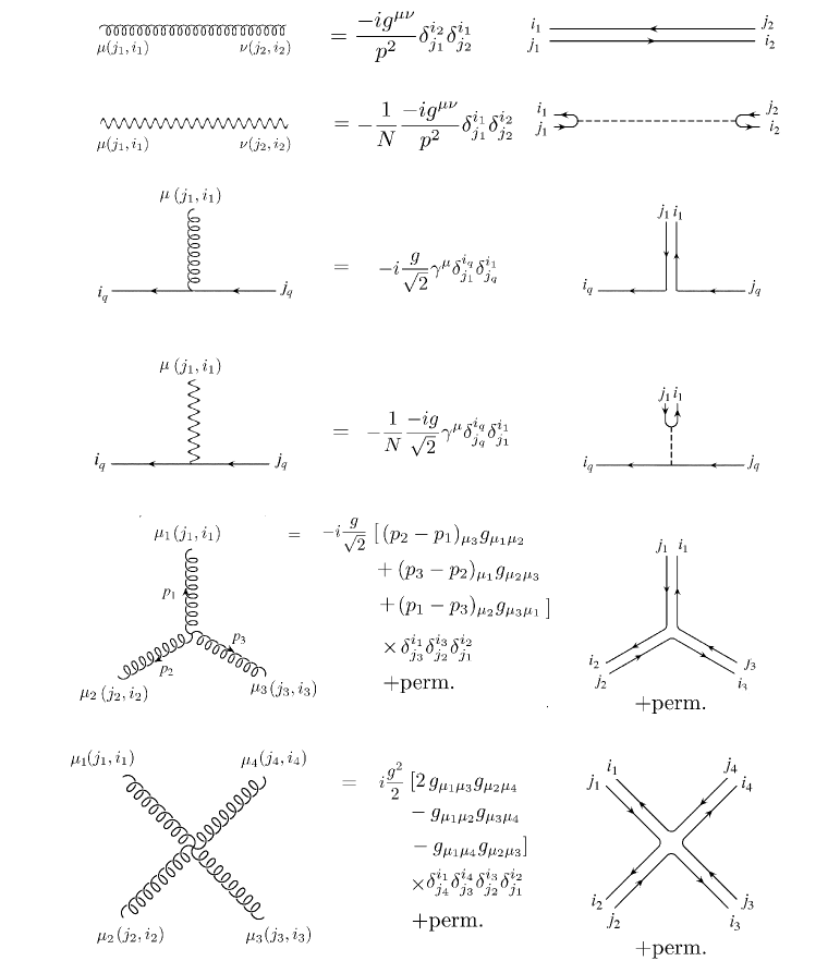
Figure 1: QCD Feynman rules in the color-flow basis. The standard Feynman diagrams are shown in the left and the color-flow diagrams are shown in the right. The wavy lines in the left and the dashed lines in the right denote the propagating Abelian gluon. The gluonic three point vertex has an additional non-cyclic permutation in color indices, while the four point vertex has additional five non-cyclic permutations.

It should be noted that both the propagator and the quark vertex of the Abelian gluon have an extra $-1/N$ factor because of the color-singlet projector, $\delta^{i}_{j}/\sqrt{N}$. The negative sign of this factor directly comes from the sign of the Abelian gluon kinetic term in the Lagrangian. We can evaluate QCD amplitudes by using these Feynman rules.

For a $n$-gluon scattering process, it is written as

$${\cal M}(ng)= \sum_{\sigma\in S_{n}/Z_{n}}\delta^{i_{\sigma(n)}}_{j_{\sigma(n-1)}}\delta^{i_{\sigma(n-1)}}_{j_{\sigma(n-2)}}\cdots\delta^{i_{\sigma(1)}}_{j_{\sigma(n)}}$$

$$\hskip 40.00006pt\times A_{\sigma}\Bigl{(}\sigma(1),\sigma(2),\cdots,\sigma(n)\Bigr{)},$$ (12)

obtained from the corresponding $n$ $U(3)$ gluon scattering process. $A_{\sigma}\Bigl{(}\sigma(1),\sigma(2),\cdots,\sigma(n)\Bigr{)}$ are gauge-invariant partial amplitudes, which depend only on particle momenta and helicities represented simply by the gluon indices, $1,\cdots,n$, and the summation is taken over all $(n-1)!$ non-cyclic permutations of gluons. A set of $n$ Kronecker delta’s in each term gives the ”color flow” of the corresponding partial amplitudes. As an example, we list in Fig. 2 all six color flows indicated by Kronecker delta’s for the $gg\rightarrow gg$ process, ${\cal G}_{j_{1}}^{i_{1}}{\cal G}_{j_{2}}^{i_{2}}\rightarrow{\cal G}_{j_{3}}^{i_{3}}{\cal G}_{j_{4}}^{i_{4}}$.

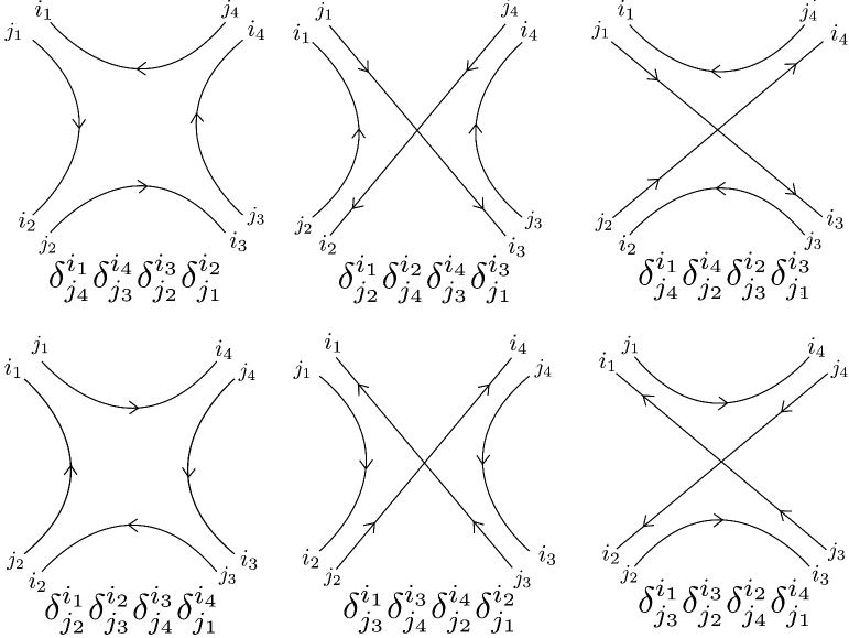
Figure 2: All 6 color flows of the process ${\cal G}_{j_{1}}^{i_{1}}{\cal G}_{j_{2}}^{i_{2}}\rightarrow{\cal G}_{j_{3}}^{i_{3}}{\cal G}_{j_{4}}^{i_{4}}$.

On the other hand, if a scattering process involves quarks, contributions from the Abelian gluon do not decouple. Therefore, we have to add all its contributions to the total amplitude. For processes with one quark line, such contributions come from Abelian gluon emitting diagrams. The total amplitude for $q\overline{q}\rightarrow ng$ process becomes

$${\cal M}(q \overline{q}+ng)$$

$$= \sum_{\sigma\in S_{n}}\delta^{i_{q}}_{j_{\sigma(n)}}\delta^{i_{\sigma(n)}}_{j_{\sigma(n-1)}}\cdots\delta^{i_{\sigma(1)}}_{j_{q}}A^{0}_{\sigma}\Bigl{(}q,\sigma(1),\cdots,\sigma(n),\overline{q}\Bigr{)}$$

$$+\sum_{\sigma\in S_{n}}\left(-\frac{1}{N}\right)\delta^{i_{\sigma(n)}}_{j_{\sigma(n)}}\delta^{i_{q}}_{j_{\sigma(n-1)}}\cdots\delta^{i_{\sigma(1)}}_{j_{q}}$$

$$\hskip 60.00009pt\times A^{1}_{\sigma}\Bigl{(}q,\sigma(1),\cdots,\sigma(n-1),\overline{q};\,\sigma(n)\Bigr{)}$$

$$+\frac{1}{2!}\sum_{\sigma\in S_{n}}\left(-\frac{1}{N}\right)^{2}\delta^{i_{\sigma(n)}}_{j_{\sigma(n)}}\delta^{i_{\sigma(n-1)}}_{j_{\sigma(n-1)}}\delta^{i_{q}}_{j_{\sigma(n-2)}}\cdots\delta^{i_{\sigma(1)}}_{j_{q}}$$

$$\hskip 20.00003pt\times A^{2}_{\sigma}\Bigl{(}q,\sigma(1),\cdots,\sigma(n-2),\overline{q};\,\sigma(n-1),\sigma(n)\Bigr{)}$$

$$\hskip 5.0pt\vdots$$

$$+\left(-\frac{1}{N}\right)^{n}\delta^{i_{n}}_{j_{n}}\cdots\delta^{i_{1}}_{j_{1}}\delta^{i_{q}}_{j_{q}}A^{n}_{\sigma}\left(q,\overline{q};\,1,\cdots,n\right),$$ (13)

where $A^{k}_{\sigma}\Bigl{(}q,\sigma(1),\cdots,\sigma(n-k),\overline{q};\,\sigma(n-k+1),\cdots,\sigma(n)\Bigr{)}$ is the partial amplitude with $k$ Abelian gluons, and $q$ and $\overline{q}$ denote the momenta and the helicities of the quark and the anti-quark, respectively. The summation is taken over all the $n!$ permutations of $n$ gluons. The first term in the r.h.s. of eq. (13) gives contributions from $n$ $U(3)$ gluons, and the other terms give contributions from $(n-k)$ $U(3)$ gluons and $k$ Abelian gluons, summed over $k=1$ to $n$, where $(-1/N)^{k}$ comes from the $-1/N$ factor in the Abelian gluon vertex as depicted in Fig. 1. Corresponding color flows of those partial amplitudes are shown in Fig. 3.

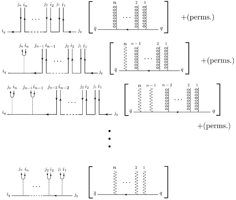
Figure 3: Color flows of $q\overline{q}\rightarrow ng$ process. For each color flow, one of the corresponding Feynman diagrams is shown in the parenthesis. The term “perms.” stands for the other color flows obtained by permutations among gluons.

For processes with two or more quark lines, the Abelian gluon can be exchanged between them, giving the amplitudes with at least $-1/N$ suppression. Therefore, the total amplitude of processes with two quark lines such as $q_{1}q_{2}\rightarrow q_{1}q_{2}+n$ gluons becomes

$${\cal M} (q_{1}\overline{q_{1}}+q_{2}\overline{q_{2}}+ng)$$

$$=\sum_{\sigma\in S_{n}}\sum_{r=0}^{n}$$

$$\left[\left(\delta^{i_{q_{1}}}_{j_{\sigma(n)}}\delta^{i_{\sigma(n)}}_{j_{\sigma(n-1)}}\cdots\delta^{i_{\sigma(r+1)}}_{j_{q_{2}}}\right)\left(\delta^{i_{q_{2}}}_{j_{\sigma(r)}}\delta^{i_{\sigma(r)}}_{j_{\sigma(r-1)}}\cdots\delta^{i_{\sigma(1)}}_{j_{q_{1}}}\right)\right.$$

$$\times A^{0}_{\sigma}\Bigl{(}q_{1},\sigma(1),\cdots,\sigma(r),\overline{q_{2}}\,|\,q_{2},\sigma(r+1),\cdots,\sigma(n),\overline{q_{1}}\Bigr{)}$$

$$-\frac{1}{N}\left(\delta^{i_{q_{2}}}_{j_{\sigma(n)}}\delta^{i_{\sigma(n)}}_{j_{\sigma(n-1)}}\cdots\delta^{i_{\sigma(r+1)}}_{j_{q_{2}}}\right)\left(\delta^{i_{q_{1}}}_{j_{\sigma(r)}}\delta^{i_{\sigma(r)}}_{j_{\sigma(r-1)}}\cdots\delta^{i_{\sigma(1)}}_{j_{q_{1}}}\right)$$

$$\Bigl{.}\times B^{0}_{\sigma}\Bigl{(}q_{1},\sigma(1),\cdots,\sigma(r),\overline{q_{1}}\,|\,q_{2},\sigma(r+1),\cdots,\sigma(n),\overline{q_{2}}\Bigr{)}\Bigr{]}$$

$$+\left({\rm partial\,\,amplitudes\,\,with\,\,external\,\,Abelian\,\,gluons}\right).$$ (14)

$A^{0}_{\sigma}\Bigl{(}q_{1},\sigma(1),\cdots,\sigma(r),\overline{q_{2}}\,|\,q_{2},\sigma(r+1),\cdots,\sigma(n),\overline{q_{1}}\Bigr{)}$ (or $B^{0}_{\sigma}$) denotes a partial amplitude with $n$ $U(3)$ gluons, where two sets of arguments divided by “$|$” belong to two different color-flow chains; one starts from $q_{1}$ ($q_{1}$ in the initial state) and ends with $\overline{q_{2}}$ ($q_{2}$ in the final state), and the other starts from $q_{2}$ and ends with $\overline{q_{1}}$, which are given explicitly by two sets of delta’s before the partial amplitude. The difference between $A^{0}_{\sigma}$ and $B^{0}_{\sigma}$ is that the former consists of $U(3)$-gluon-exchange diagrams while the latter consists of Abelian-gluon-exchange ones. Here we write down explicitly the partial amplitudes with external $U(3)$ gluons, $A^{0}$ and $B^{0}$, whereas those with external Abelian gluons should be added as in the previous one-quark-line case. For illustration, some typical diagrams for the $q_{1}q_{2}\rightarrow q_{1}q_{2}gg$ process are shown in Fig. 4.

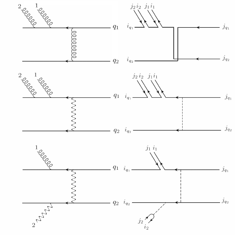
Figure 4: Sample diagrams for the $q_{1}q_{2}\rightarrow q_{1}q_{2}gg$ process. Each Feynman diagram in left-hand-side is accompanied by the corresponding color-flow diagram in the right-hand-side.

2.2 Recursive relations of off-shell gluon currents

Next, we mention the off-shell recursive relations in the color-flow basis. We define a $(n+1)$ -point off-shell gluon current $J^{\mu}(1,2,\cdots,n;\,x)$ recursively as

$$J^{\mu}(k;\,x)\equiv\delta_{j_{k}}^{\,i_{x}}\delta_{j_{x}}^{\,i_{k}}\epsilon^{\mu}(k)\hskip 10.00002pt(1\leq k\leq n),$$ (15)

$$J^{\mu} (l,l+1,\cdots,m;\,x)\hskip 20.00003pt(1\leq l<m\leq n)$$

$$\equiv\delta^{\,i_{x}}_{j_{m}}\delta^{\,i_{m}}_{j_{m-1}}\cdots\delta^{\,i_{l}}_{j_{x}}J^{\mu}(l,l+1,\cdots,m)$$

$$\equiv\frac{-i}{P^{2}_{l,m}}\Biggl{\{}\sum_{y,z}\sum_{k=l}^{m-1}\delta_{\,i_{z}}^{\,i_{x}}\delta_{\,i_{y}}^{j_{z}}\delta_{j_{x}}^{j_{y}}\,V^{\nu\rho\mu}_{3}(P_{l,k},P_{k+1,m},-P_{l,m})$$

$$\hskip 70.0001pt\times J_{\nu}(l,\cdots,k;\,y)J_{\rho}(k+1,\cdots,m;\,z)\Biggr{.}$$

$$\hskip 5.0pt+\sum_{y,z,w}\sum_{k=l}^{m-2}\sum_{q=k+1}^{m-1}\delta_{\,i_{w}}^{\,i_{x}}\delta_{\,i_{z}}^{j_{w}}\delta_{\,i_{y}}^{j_{z}}\delta_{j_{x}}^{j_{y}}\,V^{\nu\rho\sigma\mu}_{4}J_{\nu}(l,\cdots,k;\,y)$$

$$\hskip 20.00003pt\Biggl{.}\times J_{\rho}(k+1,\cdots,q;\,z)J_{\sigma}(q+1,\cdots,m;\,w)\Biggr{\}},$$ (16)

where the numbers in the argument of currents represent gluons, and their order respects the color flow as in the partial amplitudes, $A_{\sigma}$, in eq. (12); the argument after semicolon denotes the off-shell gluon. As an initial value, the 2-point gluon current, $J^{\mu}(k;\,x)$, is defined as the polarization vector of the gluon $k$, $\epsilon^{\mu}(k)$. $P_{i,j}(i<j)$ is the partial sum of gluon momenta:

$$P_{i,j}=p_{i}+p_{i+1}+\cdots+p_{j},$$ (17)

where $p_{i}$ to $p_{j}$ are defined as flowing-out momenta. $V_{3}^{\nu\rho\mu}$ and $V_{4}^{\nu\rho\sigma\mu}$ denote the three- and four-point gluon vertices from the Feynman rule of Fig. 1:

$$V_{3}^{\nu\rho\mu}(p,q,r)= -i\frac{g}{\sqrt{2}}\bigl{\{}(q-p)^{\mu}g^{\nu\rho}+(r-q)^{\nu}g^{\rho\mu}$$

$$\hskip 87.00009pt+(p-r)^{\rho}g^{\mu\nu}\bigr{\}},$$ (18)

$$V_{4}^{\nu\rho\sigma\mu}= \,\,i\frac{g^{2}}{2}(2g^{\nu\sigma}g^{\rho\mu}-g^{\nu\rho}g^{\sigma\mu}-g^{\nu\mu}g^{\rho\sigma}).$$ (19)

The summation over $y,z$ and $w$ in eq. (16) are taken over the 3 and $\overline{{\bf 3}}$ indices, $(j_{y},i_{y}),(j_{z},i_{z})$ and $(j_{w},i_{w})$, of off-shell gluons in currents $J_{\nu},J_{\rho}$ and $J_{\sigma}$, respectively. For illustration, the 5-point off-shell current is shown explicitly in Fig. 5.

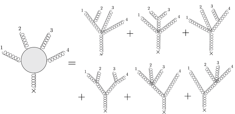
Figure 5: The 5-point gluon off-shell current. Numbers denote gluon momenta and helicities, and the curly line with $\times$ symbol denotes the off-shell gluon.

Helicity amplitudes of pure gluon processes in the color-flow basis are obtained from off-shell gluon currents as

$$\delta {}_{j_{n-1}}^{i_{n}}\delta_{j_{n-2}}^{i_{n-1}}\cdots\delta_{j_{n}}^{i_{1}}\,A(1,\cdots,n)$$

$$=\left\{\sum_{x,y,z}\sum_{k=1}^{n-2}\sum_{l=k+1}^{n-1}\delta_{i_{z}}^{j_{x}}\delta_{i_{y}}^{j_{z}}\delta_{i_{x}}^{j_{y}}\,V^{\mu\nu\rho}_{3}(P_{1,k},P_{k+1,l},P_{l+1,n})\right.$$

$$\times J_{\mu}(1,\cdots,k;\,x)J_{\nu}(k+1,\cdots,l;y)J_{\rho}(l+1,\cdots,n;\,z)$$

$$+\sum_{x,y,z,w}\sum_{k=1}^{n-3}\sum_{l=k+1}^{n-2}\sum_{m=l+1}^{n-1}\delta_{i_{w}}^{j_{x}}\delta_{i_{z}}^{j_{w}}\delta_{i_{y}}^{j_{z}}\delta_{i_{x}}^{j_{y}}\,V^{\mu\nu\rho\sigma}_{4}$$

$$\times J_{\mu}(1,\cdots,k;x)J_{\nu}(k+1,\cdots,l;y)J_{\rho}(l+1,\cdots,m;z)$$

$$\hskip 110.00017pt\Biggl{.}\times J_{\sigma}(m+1,\cdots,n;w)\Biggr{\}}.$$ (20)

Starting from the external wave functions (15), the recursive relation computes partial amplitudes very effectively by using the HELAS code. When the off-shell line “$\times$” in Fig. 5 is set on-shell, the same set of diagrams give the complete helicity amplitudes in the color-flow basis.

3 Implementation in MadGraph

In this section, we discuss how we implement off-shell recursive relations in MadGraph in the color-flow basis and how we generate helicity amplitudes of QCD processes.

3.1 Subroutines for off-shell recursive formulae

First, we introduce new HELASHELAS subroutines in MadGraph which make $n$-point gluon off-shell currents and $n$-gluon amplitudes in the color-flow basis, according to eq. (16) and eq. (20), respectively. Although the expression eq. (16) gives the off-shell gluon current made from $n$ on-shell gluons, in HELAS amplitudes any input on-shell gluon wave functions can be replaced by arbitrary off-shell gluon currents with the same color quantum numbers. Shown in Fig. 6 is an example of such diagrams that are calculated by the HELAS subroutine for the 4-point off-shell gluon current.

Figure 6: An example of the 4-point off-shell current (the external leg with the cross symbol is off-shell), where an on-shell gluon in the current (labeled as 3) is replaced by an off-shell gluon attached to a quark line.

Thanks to this property of the HELAS amplitudes, we need to introduce only two types of subroutines: one which computes helicity amplitudes of $n$-gluon processes via eq. (20) and the other which computes off-shell gluon currents from $n$-point gluon vertices via eq. (16). We name the first type of subroutines as gluon# and the second type as jgluo#, where # denotes the number of external on-shell and off-shell gluons.

The number of new subroutines we should add to MadGraph depends on the number of external partons (quarks and gluons) in QCD processes. Processes with $n$-partons can be classified as those with $n$ gluons, those with $(n-2)$ gluons and one quark line, those with $(n-4)$ gluons and two quark lines, and so on.

In the color-flow basis, the first class of processes with $n$ external gluons are calculated by just one amplitude subroutine, gluon n.

For the second class of processes with $(n-2)$ gluons and one quark line, we need up to $(n-1)$-point off-shell current subroutines, jgluo# with # $=4$ to $n-1$. This is because the largest off-shell gluon current appears in the computation of diagrams where $(n-2)$ on-shell gluons are connected to the quark line through one off-shell gluon, which can be computed by the $(n-1)$-point off-shell current and the $q\overline{q}g$ amplitude subroutine, iovxxx. Note that the same diagram can be computed by the off-shell gluon current subroutine made by the quark pair, jioxxx, and the $(n-1)$-point gluon amplitude subroutine, gluon (n-1). This type of redundancy in the computation of each Feynman diagram is inherent in the HELAS amplitudes, which is often useful in testing the codes.

For $n$-parton processes with $(n-4)$ gluons and two quark lines, we need up to $(n-2)$-point off-shell current subroutines. By also introducing multiple gluon amplitude subroutines up to $(n-2)$-point vertex, the maximum redundancy of HELAS amplitudes is achieved. Likewise, for $n$-parton processes with $m$ quark lines, we need up to $(n-m)$-point off-shell current or amplitude subroutines.

We list in Table 1 the new HELAS subroutines we introduce in this study.

gluon#	#-gluon amplitude in the color-flow basis
jgluo#	off-shell gluon current from (#$-1)$ external glu-
	ons in the color-flow basis
ggggcf	4-gluon amplitude from the contact 4-gluon ver-
	tex in the color-flow basis
jgggcf	off-shell gluon current from the contact 4-gluon
	vertex in the color-flow basis
jioaxx	off-shell Abelian gluon current from a quark pair
	in the color-flow basis

Table 1: New HELAS subroutines added into MadGraph. gluon# and jgluo# compute the #-gluon amplitude and the off-shell gluon current from the #-gluon vertex, respectively, by using the off-shell recursive formulae in the color-flow basis. We use gluon# with # $=4$ to $7$ and jgluo# with # $=4$ to $6$ in this study. Two subroutines for the contact 4-gluon vertex (ggggcf and jgggcf) are introduced to sum over the two channels ($s$ and $t$ or $s$ and $u$) for a given color flow, according to the Feynman rule in Fig. 1. We also add the off-shell Abelian gluon current subroutine from a quark pair (jioaxx).

The subroutine gluon# evaluates a #-gluon amplitude in the color-flow basis, and jgluo# computes an off-shell current from (#$-1$) external gluons. Since we consider up to seven parton processes, $gg\rightarrow 5g$, $u\overline{u}\rightarrow 5g$ and $uu\rightarrow uu3g$, in this study, we use gluon4 to gluon7 and jgluo4 to jgluo6.

In addition to these subroutines that computes amplitudes and currents recursively, we also introduce three subroutines: ggggcf, jgggcf and jioaxx. Two of them, ggggcf and jgggcf, evaluate an amplitude and an off-shell current from the contact 4-gluon vertex, following the Feynman rule of Fig. 1. Although the amplitude subroutine and the off-shell current subroutine for the 4-gluon vertex already exist in MadGraph, ggggxx and jgggxx, we should introduce the new ones which evaluate the sum of s- and t-type or s- and u-type vertices for a given color flow, since the default subroutines compute only one type at a time. jioaxx computes an off-shell Abelian gluon current made by a quark pair and is essentially the same as the off-shell gluon current subroutine, jioxxx, in the HELAS libraryHELAS except for an extra $-N$ factor:

$${\tt jioaxx}=-N\times{\tt jioxxx}.$$ (21)

Note that introducing this $-N(=-1/N\times N^{2})$ factor is equivalent to summing up contributions from all Abelian gluon propagators, as we discussed in section 2. We show the codes of ggggcf, jgggcf, gluon5 and jgluo5 in Appendix.

3.2 Introduction of a new Model: CFQCD

Next, we define a new Model with which MadGraph generates HELAS amplitudes in the color-flow basis since the present MadGraph computes them in the color-ordered basismultiparton . A Model is a set of definitions of particles, their interactions and couplings; there are about twenty preset Models in the present MadGraph packageMG/ME such as the Standard Model and the Minimal SUSY Standard ModelMSSM . There is also a template for further extension by users, User Mode (usrmod). Using this template, we can add new particles and their interactions to MadGraph. We make use of this utility and introduce a model which we call the CFQCD Model.

In the CFQCD Model, we introduce gluons and quarks as new particles labeled by indices that dictate the color flow, such that the diagrams for partial amplitudes are generated according to the Feynman rules of Fig. 1. We need one index for quarks and two indices for gluons, such as $u_{k}$, $\overline{u}_{k}$ and $g_{ji}$. The Abelian gluon, $g_{0}$, does not have an index. The index labels all possible color flows, and it runs from 1 to $m$, where

$$m={\rm the\,\,number\,\,of\,\,gluons}+{\rm the\,\,number\,\,of\,\,quark\,\,lines}.$$ (22)

This number $m$ is the number of Kronecker’s delta symbols which dictate the color flow. As an example, let us consider the purely gluonic process

$$g(1)\,g(2)\rightarrow g(3)g(4)g(5)g(6)g(7),$$ (23)

for which we need seven delta’s to specify the color flow:

$$(\delta_{7})^{i_{(7)}}_{j_{(6)}}(\delta_{6})^{i_{(6)}}_{j_{(5)}}(\delta_{5})^{i_{(5)}}_{j_{(4)}}(\delta_{4})^{i_{(4)}}_{j_{(3)}}(\delta_{3})^{i_{(3)}}_{j_{(2)}}(\delta_{2})^{i_{(2)}}_{j_{(1)}}(\delta_{1})^{i_{(1)}}_{j_{(7)}}.$$ (24)

Here the numbers in parentheses label gluons whereas the numbers in the sub-indices of Kronecker’s delta’s count the color-flow lines, 1 to $m=7$ as depicted in Fig. 7.

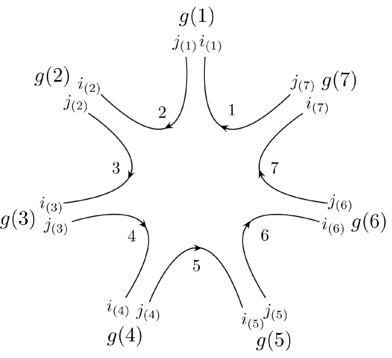
Figure 7: The color-flow diagram of the process (23) with the color flow (24). The number, 1 to 7, counts the Kronecker’s delta’s, or the color-flow lines.

In CFQCD, we label gluons according to their flowing-out, 3, and flowing-in, $\overline{{\bf 3}}$, color-flow-line numbers, such that the partial amplitude with the color flow (24) is generated as the amplitude for the process

$$g_{32}(2)\,g_{21}(1)\rightarrow g_{17}(7)\,g_{76}(6)\,g_{65}(5)\,g_{54}(4)\,g_{43}(3).$$ (25)

This is the description of the process (23) in our CFQCD Model, and we let MadGraph generate the corresponding partial amplitudes, such as $A(1,\cdots,n)$ in eq. (20), as the helicity amplitudes for the process (25). This index number assignment has one-to-one correspondence with the color flow (24). For instance, $g_{32}(2)$ in the process (25) denotes the contribution of the $U(3)$ gluon ${\cal G}^{\mu}(p_{2},\lambda_{2})_{j(2)}^{i(2)}$ to the partial amplitude where its ${\bf\bar{3}}$ index $i(2)$ terminates the color-flow line 2, and the 3 index $j(2)$ starts the new color-flow line 3. It should also be noted that we number the color-flow lines in the ascending order along the color flow, starting from the color-flow line 1 and ending with the color-flow line $m$. This numbering scheme plays an important role in defining the interactions among CFQCD gluons and quarks.

Let us now examine the case for one quark line. For the 5-jet production process

$$u\overline{u}\rightarrow g(1)\,g(2)\,g(3)\,g(4)\,g(5),$$ (26)

the color-flow index should run from 1 to 6 according to the rule (22). Indeed the color flow

$$(\delta_{6})^{i_{u}}_{j_{(5)}}(\delta_{5})^{i_{(5)}}_{j_{(4)}}(\delta_{4})^{i_{(4)}}_{j_{(3)}}(\delta_{3})^{i_{(3)}}_{j_{(2)}}(\delta_{2})^{i_{(2)}}_{j_{(1)}}(\delta_{1})^{i_{(1)}}_{j_{u}}$$ (27)

corresponds to the process

$$u_{1}\,\overline{u}_{6}\rightarrow g_{65}(5)\,g_{54}(4)\,g_{43}(3)\,g_{32}(2)\,g_{21}(1).$$ (28)

We show in Fig. 8 the color-flow diagram for this process. This is just that of the 6-gluon process cut at the $g_{16}$ gluon, where $g_{16}$ gluon is replaced by the quark pair, $u_{1}$ and $\overline{u}_{6}$. Shown in Fig. 9 are a few representative Feynman diagrams contributing to the process (28).

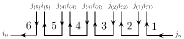
Figure 8: The color-flow diagram for $u\overline{u}\rightarrow 5g$ process. The numbers in the diagram shows the color-flow-line number.

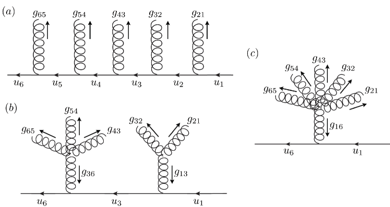
Figure 9: A few representative Feynman diagrams in the color-flow basis for the color flow of Fig. 8. Arrows indicate the quantum number flows of gluons and quarks.

Both the external and internal quarks and gluons in the CFQCD model are shown explicitly along the external and propagator lines. Following the MadGraph convention, we use flowing-out quantum numbers for gluons while the quantum numbers are along the fermion number flow for quarks. Gluon propagators attached to quark lines are named by their color-flow quantum numbers along arrows. The diagram (a) contains only $qqg$ vertices, (b) contains an off-shell 4-point gluon current, jgluo4, or a 4-point gluon amplitude, gluon4, and (c) contains either an off-shell 6-point gluon current, jgluo6, or a 6-point gluon amplitude, gluon6.

In CFQCD, not only $U(3)$ gluons but also the Abelian gluon contributes to the processes with quark lines. For the $u\overline{u}\rightarrow 5g$ process (26), 1 to 5 gluons can be Abelian gluons, $g_{0}$. If the number of Abelian gluons is $k$, the color flow reads

$$(\delta_{6})_{j_{5}}^{i_{5}}\cdots(\delta_{6-k+1})_{j_{(5-k+1)}}^{i_{(5-k+1)}}\cdot(\delta_{6-k})_{j_{(5-k)}}^{i_{u}}\cdots(\delta_{1})_{j_{u}}^{i_{(1)}}.$$ (29)

When $k=5$, all the five gluons are Abelian, and the first (the right-most) color flow should be $(\delta_{1})_{j_{u}}^{i_{u}}$, just as in $u\overline{u}\rightarrow 5$ photons. In Fig. 10, we show the color-flow diagram for the process (26) with the color flow (29) for $k=3$ as an example.

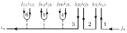
Figure 10: A color-flow diagram for $u\overline{u}\rightarrow 5g$ process with Abelian gluons. The numbers in the diagram shows the color-flow-line number.

For the process with two quark lines,

$$ud\rightarrow ud\,g(1)g(2)g(3),$$ (30)

the color-flow index should run from 1 to 5. All the possible color flows are obtained from the comb-like diagram for the one-quark-line process shown in Fig. 8, by cutting one of the gluons into a quark pair, such as $g_{k+1,k}$ to $d_{k+1}$ and $\overline{d}_{k}$. Then the first color flow starting from $u_{1}$ ends at $\overline{d}_{k}$, and the new color flow starts with $d_{k+1}$ which ends at $\overline{u}_{m}$. An example of such color flow for $k=4$ and $m=5$ reads

$$(\delta_{5})^{i_{u}}_{j_{d}}\cdot(\delta_{4})^{i_{d}}_{j_{(3)}}(\delta_{3})^{i_{(3)}}_{j_{(2)}}(\delta_{2})^{i_{(2)}}_{j_{(1)}}(\delta_{1})^{i_{(1)}}_{j_{u}}.$$ (31)

The CFQCD model computes the partial amplitude for the above color flow as the helicity amplitude for the process

$$u_{1}d_{5}\rightarrow u_{5}d_{4}\,g_{43}(3)\,g_{32}(2)\,g_{21}(1)\,.$$ (32)

The other possible color-flow processes without Abelian gluons are

$$u_{1}d_{4}\rightarrow u_{5}d_{3}\,g_{32}(2)\,g_{21}(1)\,g_{54}(3),$$ (33)

$$u_{1}d_{3}\rightarrow u_{5}d_{2}\,g_{21}(1)\,g_{54}(3)\,g_{43}(2),$$ (34)

$$u_{1}d_{2}\rightarrow u_{5}d_{1}\,g_{54}(3)\,g_{43}(2)\,g_{32}(1),$$ (35)

for $k=3,2,1$, respectively. As in the single quark line case, all the external gluons can also be Abelian gluons, and we should sum over contributions from external Abelian gluons. For instance, if the gluon $g(3)$ in the process (33) is Abelian, the color flow becomes

$$(\delta_{5})^{i_{(3)}}_{j_{(3)}}\cdot(\delta_{4})^{i_{u}}_{j_{d}}\cdot(\delta_{3})^{i_{d}}_{j_{(2)}}(\delta_{2})^{i_{(2)}}_{j_{(1)}}(\delta_{1})^{i_{(1)}}_{j_{u}},$$ (36)

and the corresponding partial amplitude is calculated for the process

$$u_{1}d_{4}\rightarrow u_{4}d_{3}\,g_{32}(2)\,g_{21}(1)\,g_{0}(3)$$ (37)

in CFQCD.

When there are more than one quark line, the Abelian gluon can be exchanged between two quark lines, and the color flow along each quark line is disconnected. For instance, the color flow

$$(\delta_{5})^{i_{d}}_{j_{(3)}}(\delta_{4})^{i_{(3)}}_{j_{d}}\cdot(\delta_{3})^{i_{u}}_{j_{(2)}}(\delta_{2})^{i_{(2)}}_{j_{(1)}}(\delta_{1})^{i_{(1)}}_{j_{u}}$$ (38)

is obtained when the Abelian gluon is exchanged between the $u$-quark and $d$-quark lines. The corresponding partial amplitude is obtained for the CFQCD process

$$u_{1}d_{4}\rightarrow u_{3}d_{5}\,g_{32}(2)\,g_{21}(1)\,g_{54}(3).$$ (39)

Note that in the process (39) each flow starts from and ends with a quark pair which belongs to the same fermion line.

We have shown so far that we can generate diagrams with definite color flow by assigning integer labels to quarks, $q_{k}$, and gluons, $g_{kl}$, such that the labels $k$ and $l$ count the color-flow lines whose maximum number $m$ is the sum of the number of external gluons and the numbers of quark lines (quark pairs), see eq. (22).

3.3 New particles and their interactions in the CFQCD Model

In Table 2, we list all the new particles in the CFQCD model for $m=6$ in eq. (22).

particle	anti-particle	type	line	mass	width	color	label	code
$U(3)$ gluons
g13	g13	V	C	ZERO	ZERO	S	g13	21
g14	g14	V	C	ZERO	ZERO	S	g14	21
g15	g15	V	C	ZERO	ZERO	S	g15	21
g16	g16	V	C	ZERO	ZERO	S	g16	21
g21	g21	V	C	ZERO	ZERO	S	g21	21
g24	g24	V	C	ZERO	ZERO	S	g24	21
g25	g25	V	C	ZERO	ZERO	S	g25	21
g26	g26	V	C	ZERO	ZERO	S	g26	21
⋮	⋮	⋮	⋮	⋮	⋮	⋮	⋮
g62	g62	V	C	ZERO	ZERO	S	g62	21
g63	g63	V	C	ZERO	ZERO	S	g63	21
g64	g64	V	C	ZERO	ZERO	S	g64	21
g65	g65	V	C	ZERO	ZERO	S	g65	21
Abelian gluon
g0	g0	V	W	ZERO	ZERO	S	g0	21
Quarks
u1	u1$\sim$	F	S	ZERO	ZERO	S	u1	2
u2	u2$\sim$	F	S	ZERO	ZERO	S	u2	2
⋮	⋮	⋮	⋮	⋮	⋮	⋮	⋮
u6	u6$\sim$	F	S	ZERO	ZERO	S	u6	2

Table 2: New particles of the CFQCD model when $m=$ the number of gluons $+$ the number of quark lines $=6$. The list is shown in the format of particles.dat in the usrmod of MadGraphMG/ME .

The list is shown in the format of particles.dat in the usrmod of MadGraphMG/ME . As explained above, the $U(3)$ gluons have two color-flow indices, $g_{kl}$, while the Abelian gluon, $g_{0}$, has no color-flow index. They are vector bosons (type$=$V), and we use curly lines (line $=$ C) for $U(3)$ gluons while wavy lines (line $=$ W) for the Abelian gluon. The ‘color’ column of the list is used by MadGraph to perform color summation by using the color-ordered basis. Since we sum over the color degrees of freedom by summing the 3 and $\overline{{\bf 3}}$ indices ($j$’s and $i$’s) over all possible color flows explicitly, we declare all our new particles as singlets (color $=$ S). The last column gives the PDG code for the particles, and all our gluons, including the Abelian gluon, are given the number 21.

All gluons, not only the Abelian gluon but also $U(3)$ gluons, are declared as Majorana particles (particle and anti-particle are the same) in CFQCD. We adopt this assignment in order to avoid generating gluon propagators between multi-gluon vertices. Such a propagator is made from a particle coming from one of the vertices and its anti-particle from the other. Since we define the anti-particle of a $U(3)$ gluon as the gluon itself, the color flow of the propagator should be flipped as shown in Fig. LABEL:fig:majoprop, according to the gluon naming scheme explained in the previous subsection. Therefore, CFQCD does not give diagrams with gluon propagator in ”color-flow conserving” amplitudes.

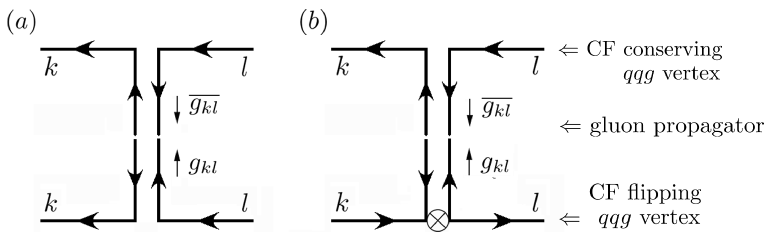
Figure 11: ’Majorana’ $U(3)$ gluon propagator in CFQCD. $k$ and $l$ denote the color-flow-line number. Since MadGraph propagator connects a flowing-out particle with a flowing-out anti-particle, it necessarily flips the color flow, as shown along the vertical lines. It either breaks the color-flow conservation, (a), and hence cannot appear inside pure gluon amplitudes, or it contributes to amplitudes with quark lines with the help of the color-flow flipping $qqg$ vertex, denoted by a cross symbol in. (b).

For example, to form a $g_{13}$ gluon propagator between two multi-gluon vertices, we need a $g_{13}$ gluon coming out from one of the vertices and a $g_{31}$ gluon from the other, according to the gluon naming scheme explained in the previous subsection. However, because a $g_{31}$ gluon is not an anti-particle of $g_{13}$ but a different particle in our particle difinition, Table 2 , $g_{13}$ gluon propagator can not be formed. $U(3)$ gluon propagators attached to quark lines are allowed by introducing the color-flow non-conserving $qqg$ couplings that effectively recover a color-flow connection. See discussions on $qqg$ vertices at the end of this section.

In Table 2, we list $u$-quarks, $u_{k}$, and its anti-particles, $\overline{u}_{k}$, with the color-flow index $k=1$ to $6$. They are all femions (type $=$ F) for which we use solid lines (line $=$ S) in the diagram. Their colors are declared as singlets (color $=$ S) as explained above. The list should be extended to the other five quarks, such as $d_{k}$ and $\overline{d}_{k}$ for down and anti-down quarks.

Before closing the explanation of new particles in CFQCD, let us note that the number of $U(3)$ gluons needed for $m$-gluon processes is $m(m-2)$. This follows from our color-flow-line numbering scheme, which counts the successive color-flow lines in the ascending order along the color flow as depicted in Fig. 7. This is necessary to avoid double counting of the same color flow. According to this rule, the only gluonic vertex possible for $m=3$ is the one among $g_{13}$, $g_{32}$ and $g_{21}$. Although $g_{31}$ can appear for processes with $m\geq 4$, $g_{12}$ and $g_{23}$ can never appear. Generalizing this rule, we find that $g_{kl}$’s with $l=k+1$ mod($m$) as well as $l=k$ cannot appear and hence we need only $m(m-2)$ gluons in CFQCD.

In this paper, we report results up to 5-jet production processes. Purely gluonic $gg\rightarrow 5g$ process has seven external gluons, and $m=7$ is necessary only for this process. According to the above rule, there is only one interaction for this process, which is the one among $g_{17}$, $g_{76}$, $g_{65}$, $g_{54}$, $g_{43}$, $g_{32}$ and $g_{21}$. Therefore, we should add $g_{17}$ and $g_{76}$ to Table 2 in order to compute $gg\rightarrow 5g$ amplitudes.

Next, we list all the interactions among CFQCD particles. Once the interactions among particles of a user defined model are given, MadGraph generates Feynman diagrams for an arbitrary process and the corresponding HELAS amplitude code. In CFQCD, we introduce $n$-point gluon interactions and let MadGraph generate a code which calls just one HELAS subroutine (either gluon# or jgluo# with # $=n$, which makes use of the recursion relations of eqs. (20) or (16), respectively) for each $n$-point vertex. In addition, we have quark-quark-gluon vertices. We list the interactions in the descending order of the number of participating particles in Table 6 to 7.

Table 3: 7-point vertices

particles	cpl1 $\cdots$ cpl5	type1 $\cdots$ type5
g17 g76 g65 g54 g43 g32 g21	G2   $\cdots$   G2	QCD   $\cdots$   QCD

Table 4: 6-point vertices

particles	cpl1 $\cdots$ cpl4	type1 $\cdots$ type4
g16 g65 g54 g43 g32 g21	G2   $\cdots$   G2	QCD   $\cdots$   QCD

Table 5: 5-point vertices

particles	cpl1  cpl2  cpl3	type1  type2  type3
g15 g54 g43 g32 g21	G2    G2    G2	QCD    QCD    QCD
g26 g65 g54 g43 g32	G2    G2    G2	QCD    QCD    QCD

Table 6: 4-point vertices

particles	cpl1 cpl2	type1 type2
g14 g43 g32 g21	G2    G2	QCD    QCD
g25 g54 g43 g32	G2    G2	QCD    QCD
g36 g65 g54 g43	G2    G2	QCD    QCD
g15 g53 g32 g21	G2    G2	QCD    QCD
g15 g54 g42 g21	G2    G2	QCD    QCD
g15 g54 g43 g31	G2    G2	QCD    QCD

Table 3 to 6: G2$=-g_{s}/\sqrt{2}$ is the coupling of gluon vertices and defined as a real, according to the HELAS convention. The list is shown in the format of interactions.dat in the usrmod of MadGraphMG/ME .

Table 7: 3-point vertices

particles	cpl	type
$g$-$g$-$g$ vertices
g13 g32 g21	G2	QCD
g24 g43 g32	G2	QCD
g35 g54 g43	G2	QCD
g46 g65 g54	G2	QCD
g14 g42 g21	G2	QCD
g14 g43 g31	G2	QCD
g15 g52 g21	G2	QCD
g15 g54 g41	G2	QCD
g25 g53 g32	G2	QCD
g25 g54 g42	G2	QCD
$q$-$q$-$g$ vertices
u1 u3 g13	GG2	QCD
u1 u3 g31	GG2	QCD
u3 u1 g31	GG2	QCD
u1 u4 g14	GG2	QCD
u1 u4 g41	GG2	QCD
u4 u1 g41	GG2	QCD
$\vdots$
u6 u7 g76	GG2	QCD
u7 u6 g76	GG2	QCD
$q$-$q$-$g_{0}$ vertices
u1 u1 g0	GG0	QCD
u2 u2 g0	GG0	QCD
$\vdots$
u6 u6 g0	GG0	QCD

G2$=-g_{s}/\sqrt{2}$, GG2$=(-g_{s}/\sqrt{2},-g_{s}/\sqrt{2})$ and GG0$=(g_{s}/(\sqrt{2}N),g_{s}/(\sqrt{2}N))$ are the couplings of each vertex. G2 is defined as a real and GG2 and GG0 are defined as two dimensional complex arrays, according to the HELAS convention. The list is shown in the format of interactions.dat in the usrmod of MadGraphMG/ME .

First, we show the 7-point interaction in Table 6 in the format of interactions.dat of usrmod in MadGraphMG/ME . As discussed above, it is needed only for generating $gg\rightarrow 5g$ amplitudes. The vertex is proportional to $g_{s}^{5}$, the fifth power of the strong coupling constant, and we give the five couplings, cpl1 to cpl5, as

$${\tt G2}=-\frac{g_{s}}{\sqrt{2}},$$ (40)

according to the Feynman rules of Fig. 1, whose types, type1 to type5, are all QCD.

The 6-point interactions appear in $gg\rightarrow 4g$ and also in $q\overline{q}\rightarrow 5g$ process in this study. Again, only one interaction is possible among the six gluons, $g_{kl}$, with $k=1$ to $6$ and $l=k-1$, as shown in Table 6. The coupling order is $g_{s}^{4}$ and the four couplings, cpl1 to cpl4, are G2 all with the type QCD.

The 5-point gluon vertices appear in $gg\rightarrow 3g$, $q\overline{q}\rightarrow 4g$, $q\overline{q}\rightarrow 5g$ and $qq\rightarrow qq\,3g$ processes. The first two and the fourth processes have $m=5$, for which the 5-point gluon vertex is unique as shown in the first row of Table 6. The process $q\overline{q}\rightarrow 5g$ gives $m=6$, and gluons with the sixth color-flow line can contribute to the 5-point gluon vertex. Because of the ascending color-flow numbering scheme, only one additional combination appears as shown in the second row of Table 6. These vertices have $g_{s}^{3}$ order and we have cpl$k=$ G2 and type$k=$ QCD for $k=1,2,3$.

The 4-point gluon vertices appear in $gg\rightarrow gg$ ($m=4$), $q\overline{q}\rightarrow(m-1)g$ with $m=4$ to $6$, and in $qq\rightarrow qq+(m-2)g$ with $m=4$ and $5$ in this study. As above, we have only one 4 -point gluon vertex for processes with $m=4$, which is shown in the first row of Table 6. For the process $q\overline{q}\rightarrow 4g$ ($m=5$), one additional vertex appears as shown in the second row. In case of $q\overline{q}\rightarrow 5g$ ($m=6$), the ordering $3\rightarrow 4\rightarrow 5\rightarrow 6$ also appears, and it is given in the third row.

So far, we obtain multiple gluon vertices from the color-flow lines of consecutive numbers, corresponding to the color flows such as

$$y+1 \rightarrow y+2\rightarrow\cdots\rightarrow y+n,$$

$$(0\leq y\leq m-n)$$ (41)

for $n$-point gluon vertices. When there are two or more quark lines in the process, we can also have color flows which skips color-flow-line numbers, such as

$$y+1\rightarrow \cdots\rightarrow y+n\rightarrow\cdots\rightarrow y+n+d,$$

$$(0\leq y\leq m-n-d),$$

$$(1\leq d\leq m-n)$$ (42)

for $n$-point gluon vertices, where $d$ counts the number of skips. Because gluon propagators do not attach to gluon vertices in CFQCD, this skip can appear only when two or more gluons from the same vertex are connected to quark lines. For example, in the fourth row of Table 6, the gluon $g_{15}$ couples to the quark line, $u_{5}\rightarrow u_{1}$, and then the gluon $g_{53}$ couples to the other quark line, $d_{3}\rightarrow d_{5}$, in the process $ud\rightarrow ud\,gg$. Likewise, $g_{42}$ and $g_{31}$ in the fifth and the sixth row, respectively, couple to the second quark line, $d\rightarrow d$, of the process.

As for the 3-gluon vertices, ten vertices listed in Table 7 appear in our study. The first four vertices with successive color-flow numbers appear in processes with one quark line, $q\overline{q}\rightarrow(m-1)g$ with $m=3$ to $6$, and those with two quark lines, $qq\rightarrow qq\,(m-2)g$ with $m=4$ to 5. The fifth and the sixth vertices starting with g14 appears for $qq\rightarrow qq\,(m-2)g$ with $m=4$, for which only one unit of skip ($d=1$) appears, and also with $m=5$. The last four vertices appear only in the $m=5$ process with two quark lines, for which $d=2$ is possible. In fact, the two vertices starting with g15 contain g52 or g41 with $d=2$ skips in the color-flow number. This completes all the gluon self-interactions in CFQCD up to 5-jet production processes.

There are two types of $qqg$ vertices in CFQCD: the couplings of $U(3)$ gluons, $g_{kl}$, and those of the Abelian gluon, $g_{0}$. All the $qqg$ couplings for the $u$-quark, $u_{1}$ to $u_{6}$, are listed in Table 7. In the HELAS convention, the fermion-fermion-boson couplings are two dimensional complex arrays, where the first and the second components are the couplings of the left- and the right-hand chirality of the flowing-in fermion. According to the Feynman rules of Fig.1, the couplings are

$${\tt GG2}=\left(-\frac{g_{s}}{\sqrt{2}},-\frac{g_{s}}{\sqrt{2}}\right)$$ (43)

for $U(3)$ gluons and

$${\tt GG0}=\left(\frac{g_{s}}{\sqrt{2}N},\frac{g_{s}}{\sqrt{2}N}\right)$$ (44)

for the Abelian gluon; Note the $-1/N$ factor for the Abelian gluon coupling.

$U(3)$ gluons have interactions as

$$u_{l}\;u_{k}\;g_{kl},$$ (45)

where the fermion number flows from $u_{l}$ to $u_{k}$ by emitting the out-going $g_{kl}$ gluon. All the diagrams with on-shell $U(3)$ gluons attached to a quark line are obtained from the vertices (45). Likewise, the Abelian gluon couples to quarks as

$$u_{k}\;u_{k}\;g_{0}.$$ (46)

In CFQCD, we generate an $U(3)$ gluon propagator between a quark line and a gluon vertex and between two quark lines by introducing color-flow flipping vertices

$$u_{k}\;u_{l}\;g_{kl}$$ (47)

as we discussed above. Here, the gluon $g_{kl}$ is emitted from the quark line $u_{k}\rightarrow u_{l}$, such that $U(3)$ gluons can propagate between a quark line and a gluonic vertex and also between two quark lines when the other side of the $qqg$ vertex is the color-flow conserving one, (45). In order to exchange gluons between an arbitrary gluonic vertex and a quark line, these color-flow-flipped $qqg$ vertices should exist for all $U(3)$ gluons. However, since all $U(3)$ gluons have the color-flow conserving vertices (45) as well, we find double counting of amplitudes where an $U(3)$ gluon is exchanged between two quark lines. This double counting can be avoided simply by discarding color–flow conserving $qqg$ vertices (45) for $k<l$ as shown in Table 7.

Now we exhaust all the interactions needed in the calculation of partial amplitudes and ready to generate diagrams and evaluate total amplitudes in the color-flow basis.

4 Total amplitudes and the color summation

In this section, we discuss how we evaluate the total amplitudes, eqs. (12), (13) and (14), with the CFQCD model and how we perform the color summation of the total amplitude squared.

4.1 $gg\rightarrow ng$ processes

We consider pure gluon processes first. As discussed in section 2, the total amplitude of a $n$-gluon process is expressed as eq. (12), and it is the sum of several partial amplitudes. Because color factors, Kronecker’s delta’s, for partial amplitudes is either 1 or 0, the total amplitude for a given color configuration (a color assignment for each external gluons) consists of a subset of all the partial amplitudes in eq. (12). Therefore, in order to evaluate the total amplitude for a given color configuration, we should find all possible color flows for the configuration, compute their partial amplitudes and simply sum them up.

As an example, let us consider a $n=5$ case,

$$g(1)g(2)\rightarrow g(3)g(4)g(5).$$ (48)

The color configuration is expressed by sets of 3 and $\overline{\bf 3}$ indices, $j$ and $i$, respectively, for each gluon;

$$(j_{1},i_{1})_{(1)},(j_{2},i_{2})_{(2)},\cdots,(j_{5},i_{5})_{(5)}.$$ (49)

Here the subscripts of each index pair label the gluon $g(k)$, $k=1$ to 5, with the momentum $p_{k}$ and the helicity $\lambda_{k}$. For instance, let us examine a color configuration

$$(1,1)_{(1)},(1,1)_{(2)},(2,1)_{(3)},(3,2)_{(4)},(1,3)_{(5)}.$$ (50)

One of the possible color flows that gives the above color configuration is

$$(\delta_{5})^{i_{(5)}}_{j_{(4)}}(\delta_{4})^{i_{(4)}}_{j_{(3)}}(\delta_{3})^{i_{(3)}}_{j_{(2)}}(\delta_{2})^{i_{(2)}}_{j_{(1)}}(\delta_{1})^{i_{(1)}}_{j_{(5)}},$$ (51)

whose associated amplitude can be calculated as the amplitude for the CFQCD process

$$g_{32}(2)\,g_{21}(1)\rightarrow\,g_{15}(5)\,g_{54}(4)\,g_{43}(3).\\$$ (52)

MadGraph generates the corresponding HELAS amplitude code, which calls the 5-gluon amplitude subroutine, gluon5.

There is also another color flow

$$(\delta_{5})^{i_{(2)}}_{j_{(5)}}(\delta_{4})^{i_{(5)}}_{j_{(4)}}(\delta_{3})^{i_{(4)}}_{j_{(3)}}(\delta_{2})^{i_{(3)}}_{j_{(1)}}(\delta_{1})^{i_{(1)}}_{j_{(2)}}$$ (53)

for the color configuration (50). The corresponding partial amplitude can be obtained by one of the $(n-1)!$ permutations of $(n-1)$ gluon momenta and helicities:

$$\bigl{\{}\epsilon^{\mu}(5),\epsilon^{\mu}(4),\epsilon^{\mu}(3),\epsilon^{\mu}(2),\epsilon^{\mu}(1)\bigr{\}}$$

$$\rightarrow \bigl{\{}\epsilon^{\mu}(2),\epsilon^{\mu}(5),\epsilon^{\mu}(4),\epsilon^{\mu}(3),\epsilon^{\mu}(1)\bigr{\}},$$ (54)

where $\epsilon^{\mu}(i)$ denotes the wave function of the external gluon $g(i)$.

When all the partial amplitudes for each color flow are evaluated, we sum them up and obtain the color-fixed total amplitude, eq. (12), for this color configuration. Therefore, for pure gluon process, we generate the HELAS amplitude once for all to evaluate the color-fixed total amplitude. The total amplitude is then squared and the summation over all color configurations is done by the Monte-Carlo method.

4.2 $q\overline{q}\rightarrow ng$ processes

Next, we discuss the processes with one quark line, $q\overline{q}\rightarrow ng$. The procedure to compute the color-summed amplitude squared is the same, but we should take into account the Abelian gluon contributions for processes with quarks. As shown in Fig. 3, the Abelian gluons appear as an isolated color index pair which have the same number. Therefore, we can take into account its contribution by regarding the independent gluon index pair as the Abelian gluon.

As an example, let us consider the process

$$u\overline{u}\rightarrow g(1)g(2)g(3)g(4)$$ (55)

with the color configuration:

$$(1,1)_{u},(1,1)_{(1)},(2,1)_{(2)},(3,2)_{(3)},(1,3)_{(4)},$$ (56)

where the parenthesis with the subscript ’$u$’ gives the color charges of the $u$-quark pair; $(j_{u},i_{u})_{u}$ denotes the annihilation of the $u$-quark with the 3 charge, $j_{u}$, and the $\overline{u}$-quark with the $\overline{\bf 3}$ charge, $i_{u}$. Although this color configuration is essentially the same as (50), and hence has the color flows like (51) and (53), we have an additional color flow for this process:

$$(\delta_{5})^{i_{(1)}}_{j_{(1)}}(\delta_{4})^{i_{u}}_{j_{(4)}}(\delta_{3})^{i_{(4)}}_{j_{(3)}}(\delta_{2})^{i_{(3)}}_{j_{(2)}}(\delta_{1})^{i_{(2)}}_{j_{u}}.$$ (57)

Here the index pair of the first gluon, $(1,1)_{(1)}$ in (56), forms an independent color flow, $(\delta_{5})^{i(1)}_{j(1)}$, which corresponds to the Abelian gluon, $g_{0}(1)$. The CFQCD process for this color flow reads

$u_{1}\overline{u}_{4}\rightarrow g_{43}(4)\;g_{32}(3)\;g_{21}(2)\;g_{0}(1)$.

Summing up, there are three color flows for the color configuration (56):

$${\rm(a)}:u\rightarrow 1\rightarrow 2\rightarrow 3\rightarrow 4\rightarrow\overline{u},$$ (58a)

$${\rm(b)}:u\rightarrow 2\rightarrow 3\rightarrow 4\rightarrow 1\rightarrow\overline{u},$$ (58b)

$${\rm(c)}:u\rightarrow 2\rightarrow 3\rightarrow 4\rightarrow\overline{u},\;1\rightarrow 1.$$ (58c)

The partial amplitude $A_{b}$ for the color flow $(b)$ is obtained from that of the color flow (a), $A_{a}$, by a permutation of gluon wave functions as in the case of $gg\rightarrow 3g$ amplitudes for the color configuration (50). The partial amplitude for the color flow $(c)$ is calculated with the Feynman rules of Fig. 1, and the total amplitude ${\cal M}$ is obtained as

$${\cal M} =A_{a}+A_{b}-\frac{1}{N}\,A_{c},$$ (59)

where the $-1/N$ factor comes from the Abelian gluon as shown in eq. (13). When more than one gluon have the same color indices, $j_{k}=i_{k}$ in $(j_{k},i_{k})_{(k)}$, more Abelian gluons can contribute to the amplitude, and the factor $\left(-1/N\right)^{m}$ appears for the partial amplitude with $m$ Abelian gluons. In the CFQCD model introduced in section 3, those factors are automatically taken into account in the HELAS code generated by MadGraph.

4.3 $qq\rightarrow qq\,(n-2)g$ processes

Finally, let us discuss the processes with two quark lines. As shown in Fig. 4, there are two independent color flows because there are two sets of quark color indices, $(j_{q_{1}},i_{q_{1}})$ and $(j_{q_{2}},i_{q_{2}})$. Nevertheless, we can show color configurations and find possible color flows in the same way as in the $q\overline{q}\rightarrow ng$ cases. Let us consider the process

$$ud\rightarrow ud\;g(1)g(2)g(3)$$ (60)

with the color configuration

$$(1,1)_{u},(1,1)_{d},(2,1)_{(1)},(3,2)_{(2)},(1,3)_{(3)}$$ (61)

for illustration. Color charges of $u$-quarks are in the parenthesis $(j_{u},i_{u})_{u}$, and those of $d$-quarks are in $(j_{d},i_{d})_{d}$ as in the $q\overline{q}\rightarrow ng$ processes. All the possible color flows are

$${\rm(a)}:\, (\delta_{5})^{i_{u}}_{j_{d}}(\delta_{4})^{i_{d}}_{j_{(3)}}(\delta_{3})^{i_{(3)}}_{j_{(2)}}(\delta_{2})^{i_{(2)}}_{j_{(1)}}(\delta_{1})^{i_{(1)}}_{j_{u}},$$ (62a)

$$\;(u\rightarrow 1\rightarrow 2\rightarrow 3\rightarrow d,d\rightarrow u)$$

$${\rm(b)}:\, (\delta_{5})^{i_{u}}_{j_{(3)}}(\delta_{4})^{i_{(3)}}_{j_{(2)}}(\delta_{3})^{i_{(2)}}_{j_{(1)}}(\delta_{2})^{i_{(1)}}_{j_{d}}(\delta_{1})^{i_{d}}_{j_{u}},$$ (62b)

$$\;(u\rightarrow d,d\rightarrow 1\rightarrow 2\rightarrow 3\rightarrow u)$$

$${\rm(c)}:\, (\delta_{5})^{i_{d}}_{j_{d}}(\delta_{4})^{i_{u}}_{j_{(3)}}(\delta_{3})^{i_{(3)}}_{j_{(2)}}(\delta_{2})^{i_{(2)}}_{j_{(1)}}(\delta_{1})^{i_{(1)}}_{j_{u}},$$ (62c)

$$\;(u\rightarrow 1\rightarrow 2\rightarrow 3\rightarrow u,d\rightarrow d)$$

$${\rm(d)}:\, (\delta_{5})^{i_{d}}_{j_{(3)}}(\delta_{4})^{i_{(3)}}_{j_{(2)}}(\delta_{3})^{i_{(2)}}_{j_{(1)}}(\delta_{2})^{i_{(1)}}_{j_{d}}(\delta_{1})^{i_{u}}_{j_{u}}.$$ (62d)

$$\;(u\rightarrow u,d\rightarrow 1\rightarrow 2\rightarrow 3\rightarrow d)$$

We show in Fig. 12 one representative Feynman diagram for each color flow, $(a)$ to $(d)$.

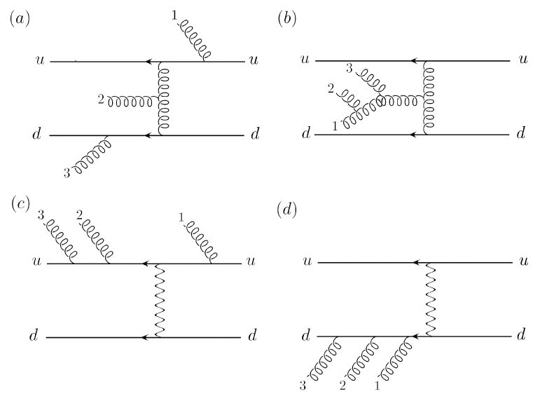
Figure 12: Feynman diagrams for the color flow (a) to (d). We show one of the Feynman diagrams for each color flow.

The amplitudes for each color flow, $A_{a}$ to $A_{d}$, are calculated as amplitudes for the corresponding CFQCD processes:

$$(a): \,u_{1}\,d_{5}\rightarrow u_{5}\,d_{4}\;g_{43}(3)\;g_{32}(2)\;g_{21}(1),$$ (63a)

$$(b): \,u_{1}\,d_{2}\rightarrow u_{5}\,d_{1}\;g_{54}(3)\;g_{43}(2)\;g_{32}(1),$$ (63b)

$$(c): \,u_{1}\,d_{5}\rightarrow u_{4}\,d_{5}\;g_{43}(3)\;g_{32}(2)\;g_{21}(1),$$ (63c)

$$(d): \,u_{1}\,d_{2}\rightarrow u_{1}\,d_{5}\;g_{54}(3)\;g_{43}(2)\;g_{32}(1).$$ (63d)

For the CFQCD processes $(c)$ and $(d)$, the color flow lines starting with the $u$- and $d$-quarks terminate at the same quarks. Such amplitudes are generated by an exchange of the Abelian gluon, as shown by the representative diagrams in Fig. 12. The total amplitude is now obtained as

$${\cal M}=A_{a}+A_{b}-\frac{1}{N}\,A_{c}-\frac{1}{N}\,A_{d},$$ (64)

according to eq. (14). The color summation of the squared amplitudes $|{\cal M}|^{2}$ is performed by the MC method just as in the pure gluon case.

5 Sample results

In this section, we present numerical results for several multi-jet production processes as a demonstration of our CFQCD model on MadGraph. We compute $n$-jet production cross sections from $gg\rightarrow ng$, $u\overline{u}\rightarrow ng$ and $uu\rightarrow uu+(n-2)g$ subprocesses up to $n=5$ in the $pp$ collision at $\sqrt{s}=14$ TeV. We define the final state cuts, the QCD coupling constant and the parton distribution function exactly as the same as those of ref. GPU2 , so that we can compare our results against those presented in ref. GPU2 , which have been tested by a few independent calculations. Specifically, we select jets (partons) that satisfy

$$|\eta_{j}|<2.5,$$ (65a)

$$p_{T}(j),\>p_{T_{jk}}>20~{}{\mbox{\rm GeV}},$$ (65b)

where $\eta_{j}$ and $p_{T}(j)$ are the pseudo-rapidity and the transverse momentum of the parton-$j$, and $p_{T_{jk}}$ is the smaller of the relative transverse momentum between parton-$j$ and parton-$k$. We use CTEQ6L1 parton distribution functionsCTEQ6L1 at the factorization scale $Q=20$ GeV and the QCD coupling $\alpha_{s}(Q=20~{}{\rm GeV})_{\overline{{\rm MS}}}=0.171$. Phase space integration and summation over color and helicity are performed by an adaptive Monte Carlo (MC) integration program BASESBASES .

Results are shown in Table 8 and Fig.13.

No. of jets	$gg\rightarrow ng$	$u\overline{u}\rightarrow ng$	$uu\rightarrow uu\,(n-2)g$
$2$	$(3.19\pm 0.00)\times 10^{11}$	$(2.90\pm 0.00)\times 10^{7}$	$(2.67\pm 0.01)\times 10^{8}$
		$(4.23\pm 0.01)\times 10^{7}$	$(3.65\pm 0.00)\times 10^{8}$
		$(2.97\pm 0.00)\times 10^{7}$	$(2.67\pm 0.01)\times 10^{8}$
$3$	$(2.61\pm 0.00)\times 10^{10}$	$(1.84\pm 0.00)\times 10^{6}$	$(5.88\pm 0.03)\times 10^{7}$
		$(2.65\pm 0.01)\times 10^{6}$	$(6.66\pm 0.04)\times 10^{7}$
		$(1.96\pm 0.01)\times 10^{6}$	$(5.93\pm 0.03)\times 10^{7}$
$4$	$(5.81\pm 0.01)\times 10^{9}$	$(4.52\pm 0.10)\times 10^{5}$	$(2.78\pm 0.02)\times 10^{7}$
		$(6.17\pm 0.01)\times 10^{5}$	$(3.03\pm 0.03)\times 10^{7}$
		$(4.78\pm 0.01)\times 10^{5}$	$(2.80\pm 0.02)\times 10^{7}$
$5$	$(4.57\pm 0.01)\times 10^{9}$	$(1.57\pm 0.03)\times 10^{5}$	$(1.54\pm 0.01)\times 10^{7}$
		$(2.13\pm 0.01)\times 10^{5}$	$(1.73\pm 0.01)\times 10^{7}$
		$(1.57\pm 0.04)\times 10^{5}$	$(1.56\pm 0.01)\times 10^{7}$

Table 8: Total cross sections of $gg\rightarrow ng$, $u\overline{u}\rightarrow ng$ and $uu\rightarrow uu+(n-2)g$ ($n\leq 5$) in fb scale for $pp$ collisions at $\sqrt{s}=14$ TeV, when jets satisfy $|\eta_{j}|<2.5$, $p_{T}(j)>20$ GeV and $p_{T_{jk}}>20$ GeV for the smaller of the relative transverse momentum between two jets. Results in the second row and the third row of each $n$-jet cross section are obtained when we ignore Abelian gluon contributions and include one Abelian gluon contributions, respectively. Abelian gluons do not contribute to purely gluonic processes.

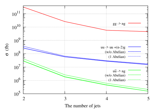
Figure 13: Total cross sections of $gg\rightarrow ng$ (upper), $uu\rightarrow uu+(n-2)g$ (middle) and $u\overline{u}\rightarrow ng$ (lower) in fb scale for $pp$ collisions at $\sqrt{s}=14$ TeV as given in Table 8. Results shown by dashed lines and dotted lines for $uu$ and $u\overline{u}$ subprocesses are obtained when Abelian gluon contributions are ignored and one Abelian gluon contributions are included, respectively.

In Table 8, the first row for each $n$-jet process gives the exact result for the $n$-jet production cross section, while the second row shows the cross section when we ignore all the Abelian gluon contributions. The third row shows the results where we include up to one Abelian gluon contributions: one Abelian gluon emission amplitudes without an Abelian gluon exchange for $u\overline{u}\rightarrow ng$ and $uu\rightarrow uu+(n-2)g$ processes, and Abelian gluon exchange amplitudes without an Abelian gluon emission for $uu\rightarrow uu+(n-2)g$ processes. All the numerical results for the exact cross sections in Table 8 agree with those presented in ref.GPU2 within the accuracy of MC integration. In Fig. 13, the multi-jet production cross sections are shown for $n=2,3,4,$ and 5 jets in units of fb. The upper line gives the results for the subprocess $gg\rightarrow ng$. The middle lines show those for the subprocess $uu\rightarrow uu+(n-2)g$; their amplitudes are obtained from those of the subprocess $ud\rightarrow ud+(n-2)g$ outlined in this study, simply by anti-symmetrizing the amplitudes with respect to the two external quark wave functions. The solid line gives the exact results, while the dashed line gives the results when all the Abelian gluon contributions are ignored. The dotted line shows the results which include up to one Abelian gluon contributions, although it is hard to distinguish from the solid line in the figure. Despite their order $1/N_{c}$ suppression, contributions of Abelian gluons can be significant; more than 30% for $n=2$, about 13% for $n=3$, while about 10% for $n=$4 and 5.

The bottom lines show results for the subprocess $u\overline{u}\rightarrow ng$. As above, the solid line gives the exact cross sections, while the dashed line and the dotted line give the results when contributions from Abelian gluons are ignored and one Abelian gluon contributions are included, respectively. Unlike the case for $uu\to uu+(n-2)g$ subprocesses, the Abelian gluon contributions remain at 30% level even for $n=5$.

Before closing this section, we would like to give two technical remarks on our implementation of CFQCD on MadGraph. First, since the present MadGraphMG/ME does not allow vertices among more than 4 particles, we add HELAS codes for 5, 6, and 7 gluon vertices by hand to complete the MadGraph generated codes. This restriction will disappear once the new version of MadGraph, MG5, is available, since MG5 accepts vertices with arbitrary number of particles. Second, we do not expect difficulty in running CFQCD codes on GPU, since all the codes we developed (see Appendix) follow the standard HELAS subroutine rules.

6 Conclusions

In this paper, we have implemented off-shell recursive formulae for gluon currents in the color-flow basis in MadGraph and have shown that it is possible to generate QCD amplitudes in the color-flow basis by introducing a new model, CFQCD, in which quarks and gluons are labeled by color-flow numbers. We have

- introduced new subroutines for off-shell recursive formulae for gluon currents, the contact 3- and 4-point gluon vertices in the color flow basis and the off-shell Abelian gluon current,
- defined new MadGraph model: the CFQCD Model,
- generated HELAS amplitudes for given color flows and calculated the color-summed total amplitude squared, and
- showed the numerical results for $n$-jet production cross sections ($n\leq 5$).

Although we have studied only up to 5-jet production processes in this paper, it is straightforward to extend the method to higher $n$-jet production processes.

Acknowledgment

We would like to thank Fabio Maltoni for his invaluable comments. This work is supported in part by the Grant-in-Aid for Scientific Research (No. 20340064) from the Japan Society for the Promotion of Science.

Appendix: Sample codes for off-shell currents and amplitudes

In this Appendix, we list HELAS codes for the contact 4-point gluon vertex subroutines, ggggcf and jgggcf, which sums over contributions with definite color-flow. In addition, we list HELAS codes for the 5-gluon amplitude subroutine, gluon5, and the 5-point off-shell gluon current subroutine, jgluo5, as examples of the recursive multi-gluon vertices introduced in section 3.

A1. ggggcf

************************************************

subroutine ggggcf(g1,g2,g3,g4,g, vertex)

implicit none

complex*16 g1(6),g2(6),g3(6),g4(6),vertex

complex*16 dv1(0:3),dv2(0:3),dv3(0:3),dv4(0:3)

complex*16 dvertx,v12,v13,v14,v23,v24,v34

real*8 g

dv1(0)=dcmplx(g1(1))

dv1(1)=dcmplx(g1(2))

dv1(2)=dcmplx(g1(3))

dv1(3)=dcmplx(g1(4))

dv2(0)=dcmplx(g2(1))

dv2(1)=dcmplx(g2(2))

dv2(2)=dcmplx(g2(3))

dv2(3)=dcmplx(g2(4))

dv3(0)=dcmplx(g3(1))

dv3(1)=dcmplx(g3(2))

dv3(2)=dcmplx(g3(3))

dv3(3)=dcmplx(g3(4))

dv4(0)=dcmplx(g4(1))

dv4(1)=dcmplx(g4(2))

dv4(2)=dcmplx(g4(3))

dv4(3)=dcmplx(g4(4))

v12= dv1(0)*dv2(0)-dv1(1)*dv2(1)-dv1(2)*dv2(2)

&      -dv1(3)*dv2(3)

v13= dv1(0)*dv3(0)-dv1(1)*dv3(1)-dv1(2)*dv3(2)

&      -dv1(3)*dv3(3)

v14= dv1(0)*dv4(0)-dv1(1)*dv4(1)-dv1(2)*dv4(2)

&      -dv1(3)*dv4(3)

v23= dv2(0)*dv3(0)-dv2(1)*dv3(1)-dv2(2)*dv3(2)

&      -dv2(3)*dv3(3)

v24= dv2(0)*dv4(0)-dv2(1)*dv4(1)-dv2(2)*dv4(2)

&      -dv2(3)*dv4(3)

v34= dv3(0)*dv4(0)-dv3(1)*dv4(1)-dv3(2)*dv4(2)

&      -dv3(3)*dv4(3)

dvertx =(-v14*v23+2.d0*v13*v24-v12*v34)

vertex = dcmplx(dvertx)*(g*g)

return

end

***********************************************

A2. jgggcf

************************************************

subroutine jgggcf(w1,w2,w3,g, jggg)

implicit none

double complex w1(6),w2(6),w3(6),jggg(6)

double complex dw1(0:3),dw2(0:3),dw3(0:3)

double complex jj(0:3),dv,w32,w13,w21,dg2

double precision q(0:3,)q2,g

double precision rOne

parameter( rOne = 1.0d0 )

jggg(5) = w1(5)+w2(5)+w3(5)

jggg(6) = w1(6)+w2(6)+w3(6)

dw1(0) = dcmplx(w1(1))

dw1(1) = dcmplx(w1(2))

dw1(2) = dcmplx(w1(3))

dw1(3) = dcmplx(w1(4))

dw2(0) = dcmplx(w2(1))

dw2(1) = dcmplx(w2(2))

dw2(2) = dcmplx(w2(3))

dw2(3) = dcmplx(w2(4))

dw3(0) = dcmplx(w3(1))

dw3(1) = dcmplx(w3(2))

dw3(2) = dcmplx(w3(3))

dw3(3) = dcmplx(w3(4))

q(0) = -dble(jggg(5))

q(1) = -dble(jggg(6))

q(2) = -dimag(jggg(6))

q(3) = -dimag(jggg(5))

q2 = q(0)**2-(q(1)**2+q(2)**2+q(3)**2)

dg2 = g*g

dv = rOne/dcmplx(q2)

w32 = dw3(0)*dw2(0)-dw3(1)*dw2(1)

&       -dw3(2)*dw2(2)-dw3(3)*dw2(3)

w13 = dw1(0)*dw3(0)-dw1(1)*dw3(1)

&       -dw1(2)*dw3(2)-dw1(3)*dw3(3)

w21 = dw2(0)*dw1(0)-dw2(1)*dw1(1)

&       -dw2(2)*dw1(2)-dw2(3)*dw1(3)

jj(0) = dg2*(-dw1(0)*w32+2d0*dw2(0)*w13

&          -dw3(0)*w21)

jj(1) = dg2*(-dw1(1)*w32+2d0*dw2(1)*w13

&          -dw3(1)*w21)

jj(2) = dg2*(-dw1(2)*w32+2d0*dw2(2)*w13

&          -dw3(2)*w21)

jj(3) = dg2*(-dw1(3)*w32+2d0*dw2(3)*w13

&          -dw3(3)*w21)

jggg(1) = dcmplx(jj(0)*dv)

jggg(2) = dcmplx(jj(1)*dv)

jggg(3) = dcmplx(jj(2)*dv)

jggg(4) = dcmplx(jj(3)*dv)

return

end

***********************************************

A3. gluon5

************************************************

subroutine gluon5 (w1,w2,w3,w4,w5,g,vertex)

implicit none

integer i

complex*16 w(6,12,12),w1(6),w2(6),w3(6),w4(6)

complex*16 w5(6),z(55),wx(6,55),vertex

real*8 g

vertex=(0d0,0d0)

do i=1,6

w(i,1,1) = w1(i)

w(i,2,2) = w2(i)

w(i,3,3) = w3(i)

w(i,4,4) = w4(i)

w(i,5,5) = w5(i)

enddo

do i=1,3

call jggxxx(w(1,i,i),w(1,i+1,i+1),g,

&                     w(1,i,i+1))

enddo

do i=1,2

call jggxxx(w(1,i,i+1),w(1,i+2,i+2),g,

&                     wx(1,1))

call jggxxx(w(1,i,i),w(1,i+1,i+2),g,wx(1,2))

call jgggcf(w(1,i,i),w(1,i+1,i+1),

&                     w(1,i+2,i+2),g,wx(1,3))

call sumw(wx,3,w(1,i,i+2))

enddo

call gggxxx(w(1,1,3),w(1,4,4),w(1,5,5),g,z(1))

call gggxxx(w(1,1,2),w(1,3,4),w(1,5,5),g,z(2))

call gggxxx(w(1,1,1),w(1,2,4),w(1,5,5),g,z(3))

call ggggcf(w(1,1,2),w(1,3,3),w(1,4,4),

&                    w(1,5,5),g,z(4))

call ggggcf(w(1,1,1),w(1,2,3),w(1,4,4),

&                    w(1,5,5),g,z(5))

call ggggcf(w(1,1,1),w(1,2,2),w(1,3,4),

&                    w(1,5,5),g,z(6))

do i=1,6

vertex = vertex+z(i)

enddo

return

end

***********************************************

A4. jgluo5

************************************************

subroutine jgluo5(w1,w2,w3,w4,g, jgluon5)

implicit none

integer i

complex*16 w(6,12,12),w1(6),w2(6),w3(6)

complex*16 w4(6),wx(6,55),jgluon5(6)

real*8 g

do i=1,6

jgluon5(i) = (0d0,0d0)

w(i,1,1) = w1(i)

w(i,2,2) = w2(i)

w(i,3,3) = w3(i)

w(i,4,4) = w4(i)

enddo

do i=1,3

call jggxxx(w(1,i,i),w(1,i+1,i+1),g,

&                     w(1,i,i+1))

enddo

do i=1,2

call jggxxx(w(1,i,i+1),w(1,i+2,i+2),g,

&                     wx(1,1))

call jggxxx(w(1,i,i),w(1,i+1,i+2),g,wx(1,2))

call jgggcf(w(1,i,i),w(1,i+1,i+1),

&                     w(1,i+2,i+2),g,wx(1,3))

call sumw(wx,3,w(1,i,i+2))

enddo

call jggxxx(w(1,1,3),w(1,4,4),g,wx(1,1))

call jggxxx(w(1,1,2),w(1,3,4),g,wx(1,2))

call jggxxx(w(1,1,1),w(1,2,4),g,wx(1,3))

call jgggcf(w(1,1,2),w(1,3,3),w(1,4,4),g,

&                    wx(1,4))

call jgggcf(w(1,1,1),w(1,2,3),w(1,4,4),g,

&                    wx(1,5))

call jgggcf(w(1,1,1),w(1,2,2),w(1,3,4),g,

&                    wx(1,6))

call sumw(wx,6,jgluon5)

return

end

***********************************************

References

- (1) T.Stelzer and W.F.Long, Comput. Phys. Commun. 81, (1994) 357.
- (2) J.Alwall, P.Demin, S.de Visscher, R.Frederix, M.Herquet, F.Maltoni, T.Plehn, D.L.Rainwaterd and T.Stelzer, JHEP 0709, (2007) 028.
- (3) K.Hagiwara, J.Kanzaki, N.Okamura, D.Rainwater, T.Stelzer, arXiv:0909.5257.
- (4) K.Hagiwara, H.Murayama and I.Watanabe, Nucl. Phys. B367, (1991) 257; H.Murayama, I.Watanabe, and K.Hagiwara, KEK-Report 91-11, (1992) 001.
- (5) K.Hagiwara, J.Kanzaki, N.Okamura, D.Rainwater, T.Stelzer, Eur. Phys. J. C66, (2009) 477.
- (6) A.Kanaki, C.G.Papadopoulos, hep-ph/0012004v1.
- (7) M.L.Mangano, M.Moretti, F.Piccinini, R.Pittau and A.D.Polosa, JHEP 0307, (2003) 001.
- (8) W.Giele, G.Stavenga, J.-C.Winter, arXiv:1002.3446[hep-ph]
- (9) F.Maltoni, K.Paul, T.Stelzer, S.Willenbrock, Phys.Rev. D 67, (2003) 014026.
- (10) F.A.Berends, W.T.Giele, Nucl. Phys. B306, (1988) 759.
- (11) M.L.Mangano, S.J.Parke, Phys. Rept. 200, (1991) 301.
- (12) G.-C.Cho, K.Hagiwara, J.Kanzaki, T.Plehn, D.Rainwater, T.Stelzer, Phys. Rev. D 73, (2006) 054002.
- (13) CTEQ Collaboration, H.L.Lai et al., Eur. Phys. J. C12, (2000) 375.
- (14) S.Kawabata, Compt. Phys. Commun. 41, (1986) 127.