Ten-moment two-fluid plasma model agrees well with PIC/Vlasov in GEM problem

Abstract

We simulate magnetic reconnection in the GEM problem using a two-fluid model with 10 moments for the electron fluid as well as the proton fluid. We show that use of 10 moments for electrons gives good qualitative agreement with the the electron pressure tensor components in published kinetic simulations.

1 Overview

This study is motivated by the following question: What is the simplest fluid model that can accurately replicate kinetic (PIC and Vlasov) simulations of fast magnetic reconnection in two-species collisionless plasma? Background for this question follows.

A plasma is a gas of charged particles interacting with an electromagnetic field. Simulations of plasma use a variety of models of plasma, which vary greatly in computational expense. For a given problem one seeks the computationally cheapest model that captures the phenomena of interest. We are specifically interested in the phenomenon of fast magnetic reconnection in “collisionless” (i.e., low-collision) plasma.

We discuss the following sequence of plasma models for two-species (e.g. electron/proton) plasmas: kinetic: Vlasov/Boltzmann or PIC (particle-in-cell), ten-moment two-fluid plasma, five-moment two-fluid plasma, and MHD (magnetohydrodynamics, a one-fluid model). Each model in this sequence can be regarded as a simplifying appoximation of its predecessor. The plasma community has used particle-in-cell (PIC) simulations as its standard first-principles plasma model. It is an approximation of the Vlasov/Boltzmann model, which we take as the “truth”. The Vlasov model is the collisionless version of the Boltzmann model. Collisionless versions of each model are hyperbolic and conserve entropy for smooth solutions, whereas collisional versions are diffusive and produce entropy.

The Geospace Environmental Modeling (GEM) Magnetic Reconnection Challenge is a benchmark magnetic reconnection problem. It was formulated to test the ability of plasma models to resolve fast magnetic reconnection in collisionless plasma. The initial GEM studies showed that PIC simulations exhibit fast reconnection, whereas reconnection is much slower in MHD (with simple resistivity) [1].

2 Plasma Models

We implemented five-moment and ten-moment two-fluid models and studied their ability to match published results of PIC and Vlasov simulations. Two-fluid models use gas-dynamics for each charged species. These fluids are coupled to Maxwell’s equations by source terms. Hakim, Loverich, and Shumlak simulated the GEM problem with a five-moment two-fluid model [6, 4] and Hakim simulated the GEM problem with a two-fluid model using 10 moments for ions and 5 moments for electrons [5], but we are unaware of any previous studies that simulate the GEM problem with a 10-moment electron fluid.

Boltzmann/Vlasov model. The Boltzmann equation asserts conservation of particle number density $f_{\mathrm{s}}(\mathbf{x},\tilde{\mathbf{v}},t)$ in phase space:

$$\partial_{t}f_{\mathrm{s}}+\nabla_{\mathbf{x}}\cdot(\mathbf{v}f_{\mathrm{s}})+\nabla_{\tilde{\mathbf{v}}}\cdot\left(\mathbf{a}f_{\mathrm{s}}\right)=C_{\mathrm{s}};$$

here $\tilde{\mathbf{v}}=\gamma\mathbf{v}\approx\mathbf{v}$ is (proper) velocity, (where $\gamma=\sqrt{1+(\tilde{v}/c)^{2}}\approx 1$ is the Lorentz factor), $\mathbf{a}=\frac{q_{\mathrm{s}}}{m_{\mathrm{s}}}(\mathbf{E}+\mathbf{v}\times\mathbf{B})$ is the acceleration due to the electric field $\mathbf{E}$ and the magnetic field $\mathbf{B}$, and $C_{\mathrm{s}}$ is a collision operator which operates on the function $(\tilde{\mathbf{v}},\mathrm{p})\mapsto f_{\mathrm{p}}(t,\mathbf{x},\tilde{\mathbf{v}})$, where $\mathrm{p}$ ranges over all species. The Vlasov equation (collisionless Boltzmann equation) asserts that $C_{\mathrm{s}}=0$. The relations $\mathbf{J}=\sum_{\mathrm{s}}q_{\mathrm{s}}\int_{\mathbf{v}}f_{\mathrm{s}}\mathbf{v}$ and $\sigma=\sum_{\mathrm{s}}q_{\mathrm{s}}\int_{\mathbf{v}}f_{\mathrm{s}}$ couple the Boltzmann equation to Maxwell’s equations

$$\partial_{t}\mathbf{B}=-\nabla\!\times\!\mathbf{E}, \nabla\!\cdot\!\mathbf{B} =0,$$

$$\partial_{t}\mathbf{E}=c^{2}\nabla\!\times\!B-\mathbf{J}/\epsilon_{0}, \nabla\!\cdot\!\mathbf{E} =\sigma/\epsilon_{0}.$$

Five-moment model. Generic physical equations for the gas-dynamic portion of the five-moment two-fluid model consist of conservation of mass and balance of momentum and energy for each species:

$$\!\!\!\!\!\!\!\!\!\!\partial_{t}\rho_{\mathrm{s}}+\nabla\!\cdot\!(\rho_{\mathrm{s}}\mathbf{u}_{\mathrm{s}})=0,$$

$$\!\!\!\!\!\!\!\!\!\!\partial_{t}(\rho_{\mathrm{s}}\mathbf{u}_{\mathrm{s}})+\nabla\!\cdot\!(\rho_{\mathrm{s}}\mathbf{u}_{\mathrm{s}}\mathbf{u}_{\mathrm{s}})+\nabla p_{\mathrm{s}}={q_{\mathrm{s}}\over m_{\mathrm{s}}}\rho_{\mathrm{s}}(\mathbf{E}+\mathbf{u}_{\mathrm{s}}\times\mathbf{B})+\mathbf{R}_{\mathrm{s}}+\nabla\!\cdot\!\underline{\underline{\sigma}}_{\mathrm{s}},$$

$$\!\!\!\!\!\!\!\!\!\!\partial_{t}\mathcal{E}_{\mathrm{s}}+\nabla\!\cdot\!(\mathbf{u}_{\mathrm{s}}(\mathcal{E}_{\mathrm{s}}+p_{\mathrm{s}}))+\nabla\!\cdot\!\mathbf{q}_{\mathrm{s}}=\nabla\!\cdot\!(\underline{\underline{\sigma}}\!\cdot\!\mathbf{u})+\mathbf{J}_{\mathrm{s}}\!\cdot\!\mathbf{E}+\mathbf{u}_{\mathrm{s}}\!\cdot\!\mathbf{R}_{\mathrm{s}}+Q^{f}_{\mathrm{s}}+Q^{t}_{\mathrm{s}},$$

where $\mathrm{s}$ is the species index ($\mathrm{i}$ for ions, $\mathrm{i}$ for electrons), $\rho_{\mathrm{s}}$ is mass density, $\mathbf{u}_{\mathrm{s}}$ is fluid velocity, $\mathcal{E}_{\mathrm{s}}$ is gas-dynamic energy, $q_{\mathrm{s}}=\pm\textrm{e}$ is particle charge, $m_{\mathrm{s}}$ is particle mass, and the species current is $\mathbf{J}_{\mathrm{s}}:=(q_{\mathrm{s}}/m_{\mathrm{s}})\rho_{\mathrm{s}}\mathbf{u}_{\mathrm{s}}$. For the pressure we assumed an isotropic monatomic gas: $(3/2)p_{\mathrm{s}}=\left(\mathcal{E}_{\mathrm{s}}-\rho_{\mathrm{s}}u_{\mathrm{s}}^{2}/2\right).$ A linear isotropic entropy-respecting viscous stress closure is $\underline{\underline{\sigma}}_{\mathrm{s}}=2\mu_{\mathrm{s}}\left(\,\mathrm{Sym}\,(\nabla\mathbf{u}_{\mathrm{s}})-\nabla\!\cdot\!\mathbf{u}_{\mathrm{s}}\mathbb{I}/3\right)$, where $\,\mathrm{Sym}\,$ denotes the symmetric part of its argument tensor, $\mathbb{I}$ is the identity tensor, and $\mu_{\mathrm{s}}$ is the shear viscosity. In these five-moment simulations, however, we neglect all collisional effects. So we neglect viscosity ($\underline{\underline{\sigma}}_{\mathrm{s}}=0$), heat flux ($\mathbf{q}_{\mathrm{s}}=0$), resistive drag force ($\mathbf{R}_{\mathrm{s}}=0$), resistive heating ($Q^{f}_{\mathrm{s}}=0$), and interspecies thermal equilibration ($Q^{t}_{\mathrm{s}}=0$). To couple these equations to Maxwell’s equations we use the relations

$$\mathbf{J} =\mathbf{J}_{i}+\mathbf{J}_{e}, \sigma =\sigma_{i}+\sigma_{e},$$

where $\sigma_{\mathrm{s}}=(q_{\mathrm{s}}/m_{\mathrm{s}})\rho_{\mathrm{s}}$ is the charge density of each species.

Ten-moment model. Generic physical equations for the gas-dynamic portion of the ten-moment two-fluid model consist of conservation of mass and balance of momentum and energy tensor for each species:

$$\partial_{t}\rho_{\mathrm{s}}+\nabla\!\cdot\!(\rho_{\mathrm{s}}\mathbf{u}_{\mathrm{s}})=0,$$

$$\partial_{t}(\rho_{\mathrm{s}}\mathbf{u}_{\mathrm{s}})+\nabla\!\cdot\!(\rho_{\mathrm{s}}\mathbf{u}_{\mathrm{s}}\mathbf{u}_{\mathrm{s}}+\mathbb{P}_{\mathrm{s}})={q_{\mathrm{s}}\over m_{\mathrm{s}}}\rho_{\mathrm{s}}(\mathbf{E}+\mathbf{u}_{\mathrm{s}}\times\mathbf{B})+\mathbf{R}_{\mathrm{s}},$$

$$\partial_{t}\mathbb{E}_{\mathrm{s}}+3\nabla\!\cdot\!\,\mathrm{Sym}\,(\mathbf{u}_{\mathrm{s}}\mathbb{E}_{\mathrm{s}})-2\nabla\!\cdot\!(\rho_{\mathrm{s}}\mathbf{u}_{\mathrm{s}}\mathbf{u}_{\mathrm{s}}\mathbf{u}_{\mathrm{s}})+\nabla\!\cdot\!\mathbbm{q}_{\mathrm{s}}$$

$$\phantom{sp}={q_{\mathrm{s}}\over m_{\mathrm{s}}}2\,\mathrm{Sym}\,(\rho_{\mathrm{s}}\mathbf{u}_{\mathrm{s}}\mathbf{E}+\mathbb{E}_{\mathrm{s}}\times\mathbf{B})+\mathbb{R}_{\mathrm{s}}+2\,\mathrm{Sym}\,(\mathbf{u}_{\mathrm{s}}\mathbf{R}_{\mathrm{s}})+\mathbb{Q}^{f}_{\mathrm{s}}+\mathbb{Q}^{t}_{\mathrm{s}},$$

where $\mathbb{E}_{\mathrm{s}}:=\int_{\mathbf{v}}f_{\mathrm{s}}\mathbf{v}\mathbf{v}$ is the energy tensor and $\mathbb{P}_{\mathrm{s}}:=\mathbb{E}_{\mathrm{s}}-\rho_{\mathrm{s}}\mathbf{u}_{\mathrm{s}}\mathbf{u}_{\mathrm{s}}$ is the pressure tensor. A linear isotropic entropy-respecting isotropization closure is $\mathbb{R}_{\mathrm{s}}=\frac{1}{\tau_{\mathrm{s}}}\left({1\over 3}(\mathrm{tr}\,\mathbb{P}_{\mathrm{s}})\mathbb{I}-\mathbb{P}_{\mathrm{s}}\right),$ where $\mathrm{tr}\,$ denotes the trace of its argument tensor and for the isotropization period we used $\tau_{\mathrm{s}}=\tau_{0}\sqrt{\frac{\det\mathbb{P}_{\mathrm{s}}}{\rho_{\mathrm{s}}^{5}}}m_{\mathrm{s}}^{3},$ which attempts to generalize the Braginskii closure; for the GEM problem this means that $\tau_{i}/\tau_{e}\approx(m_{i}/m_{e})^{5/4}$. We neglect all other collisional terms: the heat flux tensors $\mathbbm{q}_{\mathrm{s}}$, the resistive drag forces $\mathbf{R}_{\mathrm{s}}$, the frictional heating tensors $\mathbb{Q}^{f}_{\mathrm{s}}$, and the temperature equilibration tensors $\mathbb{Q}^{t}_{\mathrm{s}}$.

For small viscosity (or fast isotropization) the viscosity is related to the isotropization period by $\mu_{\mathrm{s}}\approx p_{\mathrm{s}}\tau_{\mathrm{s}}$. We set $\tau_{0}=50$. The ten-moment model offers the advantage of hyperbolic viscosity — that is, viscosity can be implemented without numerically expensive diffusive terms.

3 GEM Problem

The GEM problem is posed on a rectangular domain with periodic boundary conditions in the horizontal direction and with conducting wall boundary conditions for the upper and lower boundaries. The initial conditions are a Harris sheet equilibrium perturbed by “pinching” to form an X-point.

Nondimensionalization. The GEM problem nondimensionalizes time by the ion gyrofrequency $\Omega_{i}=\frac{eB_{0}}{m_{\mathrm{i}}}$ and the space scale by the ion inertial length $\delta_{i}$, which is the distance traveled in an ion gyroperiod $1/\Omega_{i}$ at the ion Alfvén speed $v_{A,\mathrm{i}}:=\frac{B_{0}}{\mu_{0}m_{\mathrm{i}}n_{0}}$ (where $\mu_{0}:=(c^{2}\epsilon_{0})^{-1}$ is magnetic permeability). Under this nondimensionalization the model equations above remain unchanged with the exception that $\epsilon_{0}$ is replaced by $\epsilon:=1/c^{2}$ (where $c$ is now the speed of light divided by the ion Alfvén speed).

Model Parameters. The GEM problem specifies that the ion/electron mass ratio is $m_{i}/m_{e}=25$ and the initial temperature ratio is $T_{i}/T_{e}=\sqrt{m_{i}/m_{e}}=5$. The speed of light is not specified; we used the commonly used value of $20$, chosen to be sufficiently high to exceed other wave speeds but computationally feasible.

Computational domain. The computational domain is the rectangular domain $[-L_{x}/2,L_{x}/2]\times[-L_{y}/2,L_{y}/2]$, where $L_{x}=8\pi$ and $L_{y}=4\pi$. The problem is symmetric under reflection across either the horizontal or vertical axis.

Boundary conditions. The domain is periodic in the $x$-axis. The boundaries perpendicular to the $y$-axis are thermally insulating conducting wall boundaries. A conducting wall boundary is a solid wall boundary (with slip boundary conditions in the case of ideal plasma) for the fluid variables, and the electric field at the boundary has no component parallel to the boundary. We also assume that magnetic field runs parallel to and so does not penetrate the boundary (this follows from Ohm’s law of ideal MHD, but we assume it holds generally). So at the conducting wall boundaries

$$\partial_{y}\rho_{\mathrm{s}}=0, \partial_{y}B_{x}=B_{y}=\partial_{y}B_{z}=0,$$

$$\partial_{y}u_{\mathrm{s}x}=u_{\mathrm{s}y}=\partial_{y}u_{\mathrm{s}z}=0, E_{x}=\partial_{y}E_{y}=E_{z}=0.$$

Initial conditions. The initial conditions are a perturbed Harris sheet equilibrium. The unperturbed equilibrium is given by

$$\mathbf{B}(y) =B_{0}\tanh(y/\lambda)\mathbf{e}_{x}, p(y) =\frac{B_{0}^{2}}{2n_{0}}n(y),$$

$$n_{i}(y) =n_{e}(y)=n_{0}(1/5+\,\mathrm{sech}^{2}(y/\lambda)), p_{e}(y) =\frac{T_{e}}{T_{i}+T_{e}}p(y),$$

$$\mathbf{E} =0, p_{i}(y) =\frac{T_{i}}{T_{i}+T_{e}}p(y).$$

On top of this the magnetic field is perturbed by

$$\delta\mathbf{B} =-\mathbf{e}_{z}\times\nabla(\psi),\hbox{ where}$$

$$\psi(x,y) =\psi_{0}\cos(2\pi x/L_{x})\cos(\pi y/L_{y}).$$

In the GEM problem the initial condition constants are

$$\lambda =0.5, B_{0} =1, n_{0} =1, \psi_{0} =B_{0}/10.$$

4 Method

To simulate the ten-moment and five-moment systems we implemented a Runge-Kutta Discontinuous Galerkin solver with third-order accuracy in space and time on a Cartesian mesh.

To suppress oscillations, after each time stage we limited the solution in the characteristic variables of the cell average using a modification of Krivodonova’s method (beginning with the coefficients of the highest-order Legendre basis polynomials and descending to lower order if limiting occurs) [8].

To clean the magnetic field we used a correction potential ${\psi}$ in Maxwell’s equations, as suggested in [7]:

$$\!\!\!\!\!\!\!\partial_{t}\mathbf{B}+\nabla\!\times\!\mathbf{E}{+\chi\nabla\psi}=0,\ \ \partial_{t}\mathbf{E}-c^{2}\nabla\!\times\!\mathbf{B}=-\mathbf{J}/{\epsilon_{0}},\ \ {\partial_{t}{\psi}+}{\chi c^{2}{\nabla\!\cdot\!\mathbf{B}}}={0}.$$

These equations imply a wave equation that propagates the divergence constraint error $\nabla\!\cdot\!\mathbf{B}$ at the speed $c\chi$. We used $\chi=1.05$.

Since the GEM problem is symmetric, we imposed symmetry and solved the equations on the quarter domain $[0,L_{x}/2]\times[0,L_{y}/2]$.

5 Results

We simulated the GEM problem with ten-moment and five-moment models and compared the results with the Vlasov simulations of [3] and the PIC simulations of [2]. Their plots were made at a point in time when the flux through the positive $x$-axis approximately reaches 1 nondimensionalized unit. This is shortly before the time when the reconnection rate peaks.

As measured against kinetic simulations the ten-moment model reconnects at about the correct rate and the five-moment model reconnects a bit too quickly, perhaps because in the five-moment model compression in the outflow direction automatically causes increased pressure in the perpendicular directions, opening up the outflow region and artificially increasing the rate of reconnection.

In contrast to the five-moment model the ten-moment model is capable of representing an anisotropic pressure tensor. Our plots of the ten-moment electron pressure tensor components look like somewhat smudged versions of the corresponding plots for the Vlasov model.

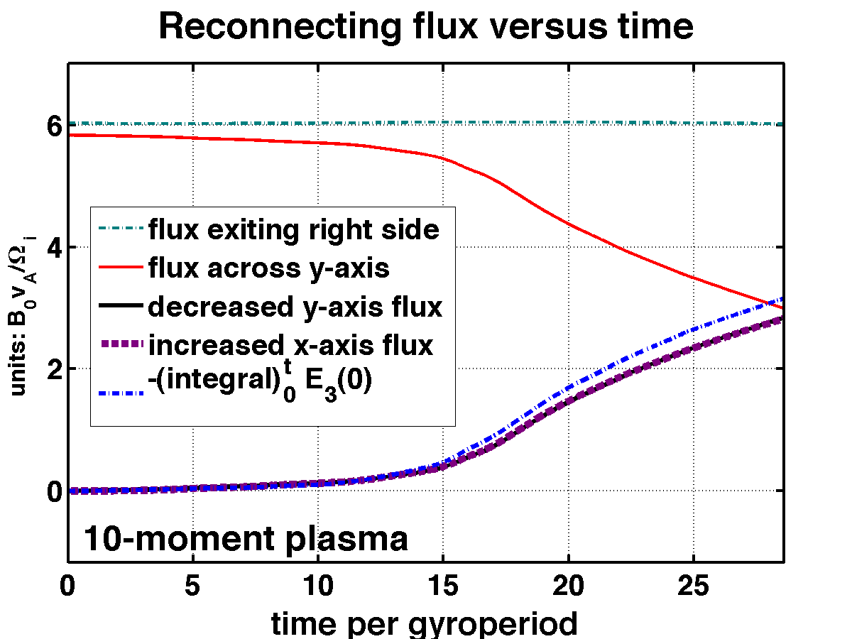
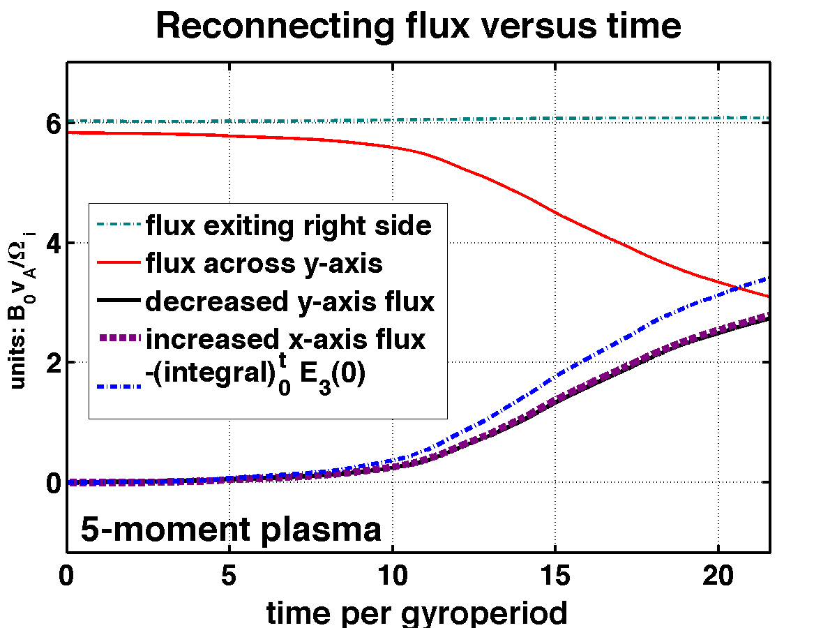
Figure 5.1: Ramp-up of reconnected flux for 10-moment and 5-moment plasma. Fluxes are through the boundaries of the first quadrant of the domain. In each model the bottom three lines should coincide. Times at which the magnetic flux through the positive $x$-axis reached one nondimensionalized unit per model were $17.2$ (our 10-moment) $13.0$ (our 5-moment), $17.7$ (Vlasov [3]), $15.7$ (PIC [2]), $17.6$ (10/5-moment [5]), $15.6$ (5-moment [4]) and $15.3$ (5-moment [6]).

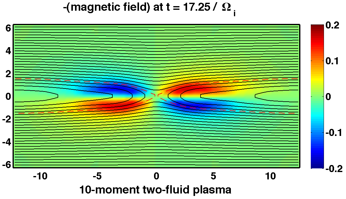
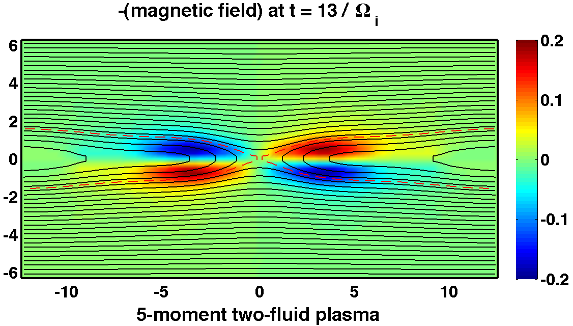
Figure 5.2: Magnetic field when one unit of flux passes through the positive $x$-axis. These results compare well with Plate 1 of [2] and the magnetic field shown in FIG. 2 of [3].

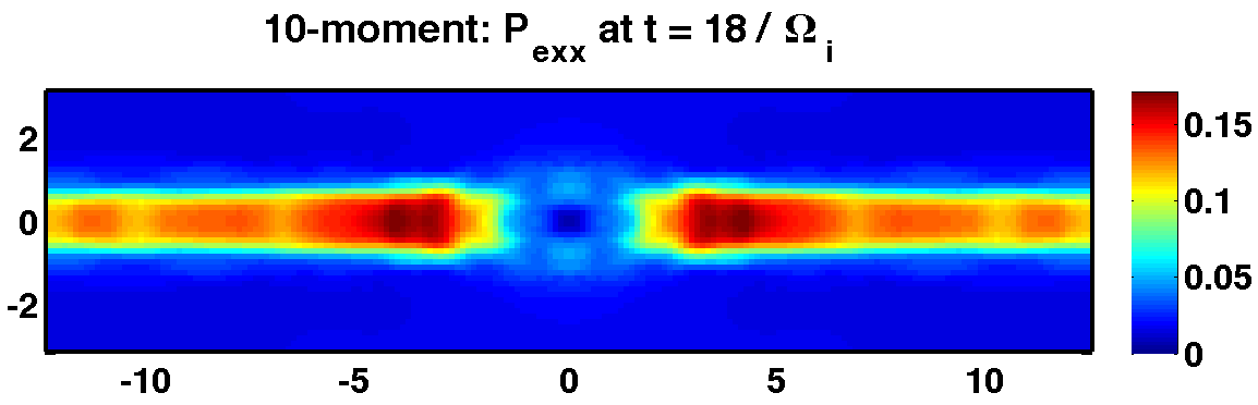
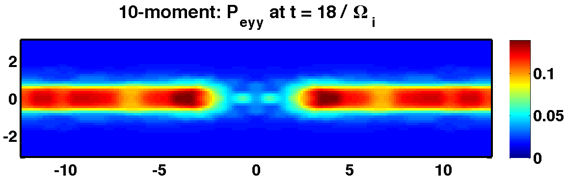
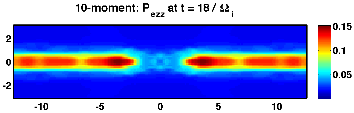
Figure 5.3: Diagonal components of the electron pressure tensor for 10-moment simulation at $\Omega_{i}t=18$. These look like smudged versions of the plots in FIG. 5 of [3].

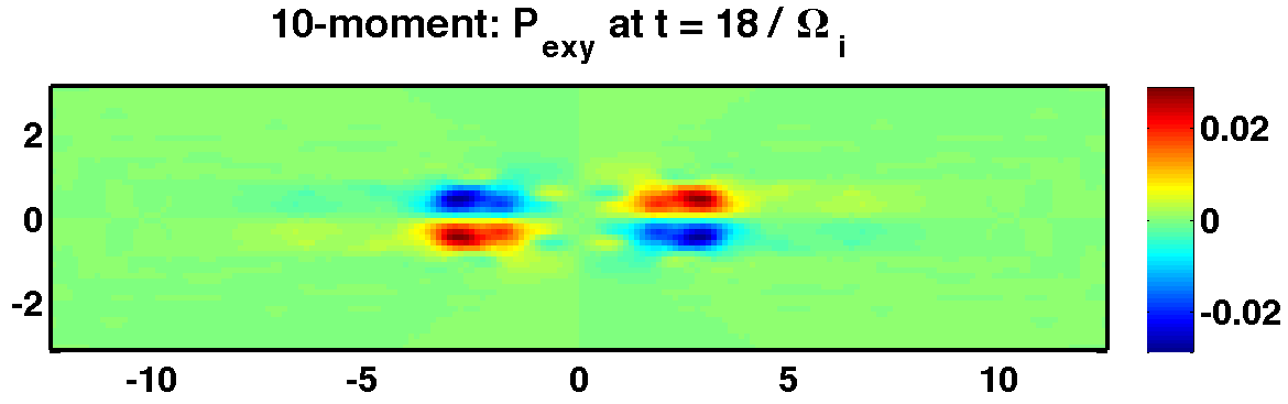
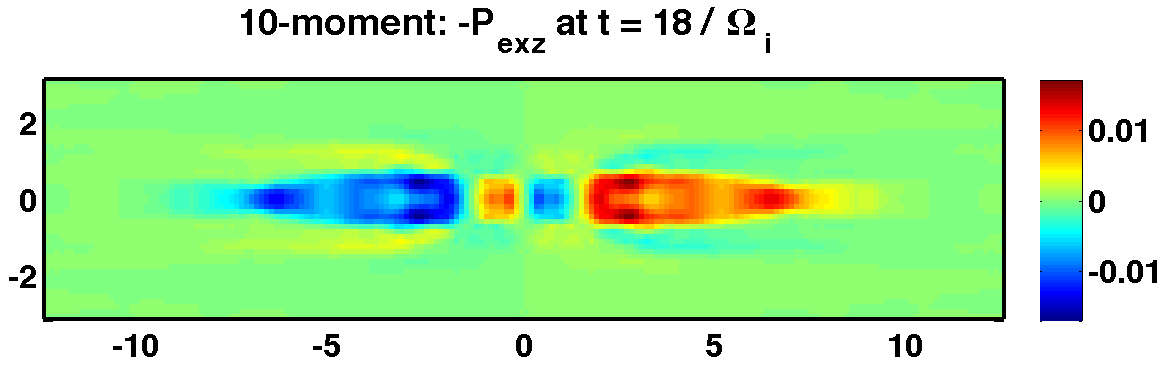
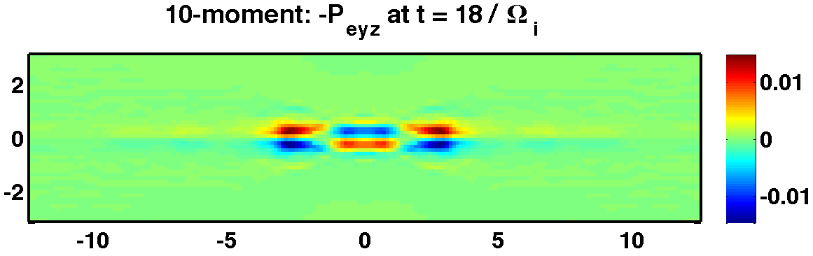
Figure 5.4: Off-diagonal components of the electron pressure tensor for 10-moment simulation at $\Omega_{i}t=18$. These look like smudged versions of the plots in FIG. 6 of [3].

References

• [1] J. Birn, J.F. Drake, M.A. Shay, B.N. Rogers, R.E. Denton, M. Hesse, M. Kuznetsova, Z.W. Ma, A. Bhattacharjee, A. Otto, and P.L. Pritchett. Geospace environmental modeling (GEM) magnetic reconnection challenge. Journal of Geophysical Research – Space Physics, 106:3715–3719 (2001).
• [2] P. L. Pritchett. Geospace Environment Modeling magnetic reconnection challenge: Simulation with a full particle electromagnetic code. Journal of Geophysical Research, vol. 106, no. A3, pp. 3783–3798 (2001).
• [3] H. Schmitz and R. Grauer. Kinetic Vlasov simulations of collisionless magnetic reconnection. Physics of Plasmas, 13, 092309 (2006).
• [4] A. Hakim, J. Loverich, and U. Shumlak. A high-resolution wave propagation scheme for ideal two-fluid plasma equations. J. Comp. Phys., 219:418–442 (2006).
• [5] A.H. Hakim. Extended MHD modelling with the ten-moment equations. J. Fusion Energy, 27:36–43 (2008).
• [6] J. Loverich, A. Hakim, U. Shumlak. A Discontinuous Galerkin Method for Ideal Two- Fluid Plasma Equations. Submitted to Physics of Plasmas, posted at arXiv:1003.4542v1 (2010).
• [7] A. Dedner, F. Kemm, D. Kröner, C.-D. Munz, T. Schnitzer, and M. Wesenberg. Hyperbolic divergence cleaning for the MHD equations. J. Comp. Phys., 175:645-673 (2002).
• [8] L. Krivodonova. Limiters for high-order discontinuous Galerkin methods. J. Comp. Phys., 226:879–896 (2007).