Measuring spin and ${\cal{CP}}$ from semihadronic $ZZ$ decays using jet substructure

Abstract

We apply novel jet techniques to investigate the spin and ${\cal{CP}}$ quantum numbers of a heavy resonance $X$, singly produced in $pp\rightarrow X\rightarrow ZZ\rightarrow\ell^{+}\ell^{-}jj$ at the LHC. We take into account all dominant background processes to show that this channel, which has been considered unobservable until now, can qualify under realistic conditions to supplement measurements of the purely leptonic decay channels $X\rightarrow ZZ\rightarrow 4\ell$. We perform a detailed investigation of spin- and ${\cal{CP}}$-sensitive angular observables on the fully-simulated final state for various spin and ${\cal{CP}}$ quantum numbers of the state $X$, tracing how potential sensitivity communicates through all the steps of a subjet analysis. This allows us to elaborate on the prospects and limitations of performing such measurements with the semihadronic final state. We find our analysis particularly sensitive to a ${\cal{CP}}$-even or ${\cal{CP}}$-odd scalar resonance, while, for tensorial and vectorial resonances, discriminative features are diminished in the boosted kinematical regime.

I Introduction

An experimental hint pointing towards the source of electroweak symmetry breaking (EWSB) remains missing. From a theoretical perspective, unitarity constraints do force us to expect new physics manifesting at energy scales $\lesssim 1.2~{}{\rm{TeV}}$. For most of the realistic new physics models, this effectively means the observation of at least a single new resonant state in the weak boson scattering (sub)amplitudes, which serves to cure the bad high-energy behavior of massive longitudinal gauge boson scattering. An equal constraint does also follow from diboson production from massive quarks, $q\bar{q}\rightarrow W^{+}W^{-}$, which relates EWSB to the dynamics of fermion mass generation cornwall . Revealing the unitarizing resonance’s properties, such as mass, spin and ${\cal{CP}}$ quantum numbers, is a primary goal of the CERN Large Hadron Collider (LHC) Aad:2008zzm ; Ball:2007zza . Completing this task will provide indispensable information elucidating the realization of EWSB and will therefore help to pin down the correct mechanism of spontaneous symmetry breaking.

At the LHC, the experimentally favorite channel to determine ${\cal{CP}}$ and spin of a new massive particle $X$ ($m_{X}\gtrsim 300~{}{\rm{GeV}}$), coupling to weakly charged gauge bosons, is its decay to four charged leptons via $X\rightarrow ZZ$ Buszello:2002uu ; Buszello:2004uu ; Gao:2010qx ; DeRujula:2010ys ; Choi:2002jk . These “golden channels” goldplatedmode are characterized by extraordinarily clean signatures, making them experimentally well-observable at, however, small rates due to the small leptonic $Z$ branching ratios. Until now, $X\rightarrow ZZ$ for the semihadronic decay channels $ZZ\rightarrow\ell^{+}\ell^{-}jj$ has been considered experimentally disfavored. In part, this is due to the overwhelmingly large backgrounds from underlying event and quantum chromodynamics (QCD), which exceed the expected signal by a few orders of magnitude. An analogous statement has been held true for associated standard model Higgs production, until, only very recently, new subjet techniques have proven capable of discriminating signal from background for highly boosted Higgs kinematics Butterworth:2008iy ; Plehn:2009rk ; Soper:2010xk . Subsequently, these phase space regions have received lots of attention in phenomenological analysis, demonstrating the capacity of subjet-related searches at the LHC in various channels and models subjets . $H\rightarrow WW$ was one of the first channels subjet techniques were ever applied to Seymour:1993mx . The purpose of these analysis was predominantly to isolate a resonance peak from an invariant mass distribution. In this paper we use a combination of different subjet methods for a shape-analysis of spin- and ${\cal{CP}}$-sensitive observables in a semihadronic final state. ${\cal{CP}}$ properties of the standard model (SM)-like associated Higgs production have been investigated recently in Ref. Christensen:2010pf using $b$-tagging in $HZ\rightarrow\ell^{+}\ell^{-}b\bar{b}$.

Subjet techniques have also proven successful in $pp\rightarrow X\rightarrow ZZ\rightarrow\ell^{+}\ell^{-}jj$ for standard model-like Higgs production ($X=H$ with $m_{H}\gtrsim 350~{}{\rm{GeV}}$) in Ref. Hackstein:2010wk , yielding a $5\sigma$ discovery reach for an integrated luminosity of $10~{}{\rm{fb}}^{-1}$, when running the LHC at a center-of-mass energy of $\sqrt{s}=14~{}{\rm{TeV}}$. Equally important, the semihadronic decay channel exhibits a comparable statistical significance as the purely leptonic channels $pp\rightarrow X\rightarrow ZZ\rightarrow\ell\ell\ell^{\prime}\ell^{\prime}$. This can be of extreme importance if the LHC is not going to reach its center-of-mass design-energy. Hence, there is sufficient potential to revise semihadronic decays, not only to determine the resonance mass, but also its spin- and ${\cal{CP}}$ properties.

The main goal of this paper is to investigate the attainable extent of sensitivity to the spin and ${\cal{CP}}$ quantum numbers of a resonance $X$ in the channel $pp\rightarrow X\rightarrow ZZ\rightarrow\ell^{+}\ell^{-}jj$, for the selection cuts, which allow to discriminate the signal from the background. To arrive at a reliable assessment, we take into account realistic simulations of both the signal and the dominating background processes. We fix the mass and the production modes of $X$, as well as its production cross section to be similar to the SM Higgs boson expectation. On the one hand, this approach can be motivated by again referring to unitarity constraints: Curing the growth of both the $VV\rightarrow VV$ and $q\bar{q}\rightarrow WW$ scattering amplitudes by a singly dominating additional resonance fixes the overall cross section to be of the order of the SM (see e.g. Duhrssen:2004cv ; Birkedal:2004au for non trivial examples). On the other hand, we would like to focus on an experimental situation, which favors the SM expectation, but leaving ${\cal{CP}}$ and spin properties as an open question. For this reason, we also do not include additional dependencies of the cross section on the width of $X$. The width is, in principle, an additional, highly model-dependent parameter, which can be vastly different from the SM Higgs boson width (e.g. in models with EWSB by strong interactions Chanowitz:1985hj ; silh or in so-called hidden-valley models Strassler:2006im ). Instead, we straightforwardly adopt the SM Higgs boson width, which then turns the resonance considered in this paper into a “Higgs look-alike”, to borrow the language of Ref. DeRujula:2010ys .

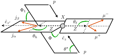
Figure 1: Spin- and ${\cal{CP}}$-sensitive angles of Ref. Dell'Aquila:1985ve in $pp\rightarrow X\rightarrow ZZ\rightarrow\mu^{+}\mu^{-}jj$. Details on the angles’ definition and on the assignment of $j_{\alpha}$ and $j_{\beta}$ are given in the text. An angle analogous to $\Phi_{1}$ can be defined with respect to the leptonic decay plane. We refer to this angle as $\tilde{\Phi}$.

We organize this paper as follows: In Sec. II, we outline the necessary technical details of our analysis. We review the effective interactions, from which we compute the production and the decay of the resonance $X$ with quantum numbers $J^{CP}=0^{\pm},1^{\pm},2^{+}$. We also comment on the signal and background event generation and the chosen selection criteria, and we introduce the ${\cal{CP}}$ and spin-sensitive observables and their generalization to semihadronic final states. We discuss our numerical results in Sec. III; Sec. IV closes with a summary and gives our conclusions.

II Details of the analysis

II.1 Spin- and ${\cal{CP}}$-sensitive observables

The spin and ${\cal{CP}}$ properties are examined through correlations in the angular distributions of the decay products. A commonly used (sub)set of angles is given by the definitions of Cabibbo and Maksymowicz of Ref. Cabibbo:1965zz , which originate from similar studies of the kaon system (see, e.g., Refs. DeRujula:2010ys ; Buszello:2002uu ; Bredenstein:2006rh ; Cao:2009ah for their application to the $X\rightarrow ZZ$). In this paper we focus on the angles of Ref. Dell'Aquila:1985ve as sensitive observables, which also have been employed in the recent $X\rightarrow 4l$ investigation in Ref. Gao:2010qx . We quickly recall their definition with the help of Fig. 1: Let ${\bf{p}}_{\alpha},~{}{\bf{p}}_{\beta}$, and ${\bf{p}}_{\pm}$ be the three-momenta of the (sub)jets $j_{\alpha}$ and $j_{\beta}$ and the leptons in the laboratory frame, respectively. From these momenta, we compute the three-momenta of the hadronically and leptonically decaying $Z$ bosons

$${\bf{p}}_{Z_{h}}={\bf{p}}_{\alpha}+{\bf{p}}_{\beta}\,,\qquad{\bf{p}}_{Z_{\ell}}={\bf{p}}_{+}+{\bf{p}}_{-}\,,$$ (1a)

as well as the lab-frame $$X$$ three-momentum

$${\bf{p}}_{X}={\bf{p}}_{\alpha}+{\bf{p}}_{\beta}+{\bf{p}}_{+}+{\bf{p}}_{-}\,.$$ (1b)

In addition, we denote the normalized unit vector along the beam axis measured in the $$X \hat{e}_{z} ZZ X \hat{e}_{z^{\prime}}$$ rest frame by , and the unit vector along the decay axis in the rest frame by . The angles of Fig. 1 are then defined as follows

$$\cos\theta_{h}= {{\bf{p}}_{\alpha}\cdot{\bf{p}}_{X}\over\sqrt{{\bf{p}}^{2}_{\alpha}\,{\bf{p}}^{2}_{X}}}\bigg{|}_{Z_{h}}, \cos\theta_{\ell}= {{\bf{p}}_{-}\cdot{\bf{p}}_{X}\over\sqrt{{\bf{p}}^{2}_{-}\,{\bf{p}}^{2}_{X}}}\bigg{|}_{Z_{\ell}},$$ (1c)

$$\cos\theta^{\star}= {{\bf{p}}_{Z_{\ell}}\cdot{\hat{e}_{z^{\prime}}}\over\sqrt{{\bf{p}}^{2}_{Z_{\ell}}}}\bigg{|}_{X}, \cos\tilde{\Phi}= {(\hat{e}_{z}\times\hat{e}_{z^{\prime}})\cdot({\bf{p}}_{-}\times{\bf{p}}_{+})\over\sqrt{({\bf{p}}_{-}\times{\bf{p}}_{+})^{2}}}\bigg{|}_{X},$$ (1d)

$$\cos\Phi={({\bf{p}}_{\alpha}\times{\bf{p}}_{\beta})\cdot({\bf{p}}_{-}\times{\bf{p}}_{+})\over\sqrt{({\bf{p}}_{\alpha}\times{\bf{p}}_{\beta})^{2}\,({\bf{p}}_{-}\times{\bf{p}}_{+})^{2}}}\bigg{|}_{X}\,,$$ (1e)

where the subscripts indicate the reference system, in which the angles are evaluated. More precisely, the helicity angles $\theta_{h}$ and $\theta_{\ell}$ are defined in their mother-$Z$’s rest frame, and all other angles are defined in the rest frame of the particle $X$, where ${\bf{p}}_{Z_{\ell}}=-{\bf{p}}_{Z_{h}}$. It is also worth noting that the helicity angles correspond to the so-called Collins-Soper angle of Ref. Collins:1977iv , evaluated for the respective $Z$ boson.

There is a small drawback when carrying over the definitions of Eq. (1) from the purely leptonic decay channels to the considered semihadronic final state: When dealing with $X\rightarrow\ell^{+}\ell^{-}\ell^{\prime+}\ell^{\prime-}$, it is always possible to unambiguously assign a preferential direction for the lepton pairs by tagging their charge. This allows us to fix a convention for the helicity angles, as well as for the relative orientation of the decay planes via a specific order of the three-momenta when defining the normal vectors in Eq. (1). Considering semihadronic $X$ decays, we are stuck with a twofold ambiguity, which affects the angular distributions. Even worse, $p_{T}$-ordered hard subjets, dug out from the “fat jet” during the subjet analysis (for details see Sec. II.3) can bias the distributions. Hence, we need to impose an ordering scheme which avoids these shortcomings. An efficiently working choice on the inclusive parton level is provided by the imposing rapidity-ordering

$$y(j_{\alpha})<y(j_{\beta})\,,$$ (2)

which is reminiscent of the ${\cal{CP}}$-sensitive $\Phi_{jj}$ observable in vector boson fusion Hankele:2006ma . This choice, however, does not remove all ambiguities. The orientation of the decay planes [Eq. (1e)] is not fixed by ordering the jets according to Eq. (2). The unresolved ambiguity results in averaging $\cos\Phi$ and $\cos(\pi-\Phi)$ over the event sample, leaving a decreased sensitivity in the angle $\Phi\in[0,\pi]$. We discuss this in more detail in Sec. III.

II.2 Simulation of signal and background events

We generate signal events $pp\rightarrow X\rightarrow ZZ\rightarrow\ell^{+}\ell^{-}jj$ with MadGraph/MadEvent Alwall:2007st , which we have slightly modified to fit the purpose of this work. In particular these modifications include supplementing additional Helas Murayama:1992gi routines and modifications of the MadGraph-generated code to include vertex structures and subprocesses that are investigated in this paper. We have validated our implementation against existing spin correlation results of Refs. Djouadi:2005gi ; Gao:2010qx . We choose the partonic production modes to be dependent on the quantum numbers of the particle $X$:

$$X=0^{\pm}: \quad gg\rightarrow X\rightarrow ZZ\rightarrow\ell^{+}\ell^{-}jj\,,$$ (3a)

$$X=1^{\pm}: \quad q\bar{q}\rightarrow X\rightarrow ZZ\rightarrow\ell^{+}\ell^{-}jj\,,$$ (3b)

$$X=2^{+}: \quad gg\rightarrow X\rightarrow ZZ\rightarrow\ell^{+}\ell^{-}jj\,,$$ (3c)

where $g$ denotes the gluon and $q,j=(u,d,s,c)$ represents the light constituent quarks of the proton.

The bottom quark contributions are negligibly small. While, in the light of the effective theory language of Ref. Gao:2010qx , this specific choice can be considered as a general assumption of our analysis, the partonic subprocesses of Eq. (3) reflect the dominant production modes at the LHC. In particular, the production of an uncolored vector particle $1^{-}$ from two gluons via fermion loops is forbidden by Furry’s theorem furrythrm , while a direct $ggZ^{\prime}$ coupling is ruled out by Yang’s theorem Yang:1950rg .

The effective operators that we include for the production and the decay of $X$ do not exhaust all possibilities either (see again Ref. Gao:2010qx for the complete set of allowed operators). Yet, we adopt a general enough set of operators to adequately highlight the features of objects $X$ with different spins and ${\cal{CP}}$ quantum numbers in our comparative investigation in Sec. III. The effective vertex function, from which we derive the effective couplings of $X$ to the SM $Z$ bosons, that appear in the calculation of the matrix elements in Eq. (3), reads for the scalar case suppressing the color indices Hagiwara:1986vm ,

$${\cal{L}}^{ZZX}_{\mu\nu}=c^{s}_{1}\,g_{\mu\nu}+{c_{2}^{s}\over m_{Z}^{2}}\epsilon_{\mu\nu\rho\delta}\,p_{1}^{\rho}\,p_{2}^{\delta}\,.$$ (4a)

For a vectorial $$X$$, the vertex function follows from the generalized Landau-Yang theorem Keung:2008ve

$${\cal{L}}^{ZZX}_{\mu\nu\rho}=c^{v}_{1}\left(g_{\mu\rho}\,p_{1,\nu}+g_{\nu\rho}\,p_{2,\mu}\right)\\ -c^{v}_{2}\,\epsilon_{\mu\nu\rho\delta}\left(p_{1}^{\delta}-p_{2}^{\delta}\right),$$ (4b)

while for tensorial $$X$$, we include the vertex function spin2

$${\cal{L}}^{ZZX}_{\mu\nu\rho\delta}=c_{1}^{t}\big{(}p_{1,\nu}\,p_{2,\rho}\,g_{\mu\delta}+p_{1,\rho}\,p_{2,\mu}\,g_{\nu\delta}\\ +p_{1,\rho}\,p_{2,\delta}\,g_{\mu\nu}-{1\over 2}m_{X}^{2}\,g_{\mu\rho}\,g_{\mu\delta}\big{)}$$ (4c)

to our comparison.

From Eqs. (4), we can determine the (off-shell) decays $X,X_{\rho},X_{\rho\delta}\rightarrow Z_{\mu}(p_{1})Z_{\nu}(p_{2})$ by contracting with the final state $Z$ bosons’ effective polarization vectors $\varepsilon^{\ast}_{\mu}(p_{1})$ and $\varepsilon^{\ast}_{\nu}(p_{2})$, which encode the Breit-Wigner propagator and the respective $Z$ decay vertex.

	$0^{+}$		$0^{-}$		$1^{-}$		$1^{+}$		$2^{+}$		$Z+\rm{jets}$		$ZZ$		$t\bar{t}$
	P	H	P	H	P	H	P	H	P	H	P	H	P	H	P	H
Raw	1.00		1.00		1.00		1.00		1.00		1.00		1.00		1.00
Cuts	0.41	0.53	0.35	0.47	0.28	0.40	0.29	0.42	0.31	0.40	0.15	0.17	0.24	0.36	0.02	0.01
Hadr.$Z$	0.22	0.29	0.16	0.22	0.16	0.22	0.16	0.23	0.15	0.19	4.2$\times 10^{-3}$	6.5$\times 10^{-3}$	0.02	0.03	1.2$\times 10^{-3}$	0.8$\times 10^{-3}$
$m_{X}$	0.17	0.22	0.12	0.16	0.12	0.17	0.13	0.18	0.11	0.15	1.6 $\times 10^{-3}$	2.2$\times 10^{-3}$	4.7$\times 10^{-3}$	7.0$\times 10^{-3}$	2.3$\times 10^{-4}$	1.6$\times 10^{-4}$
$\Delta R_{ZZ}$	0.15	0.20	0.11	0.14	0.10	0.14	0.10	0.14	0.10	0.13	1.3 $\times 10^{-3}$	1.9 $\times 10^{-3}$	3.7$\times 10^{-3}$	5.7 $\times 10^{-3}$	2.0$\times 10^{-4}$	1.3$\times 10^{-4}$
Tr+Pr	0.10	0.13	0.07	0.09	0.07	0.10	0.07	0.10	0.06	0.08	4.7 $\times 10^{-4}$	5.7$\times 10^{-4}$	1.9$\times 10^{-3}$	2.9$\times 10^{-3}$	7.8$\times 10^{-5}$	4.2$\times 10^{-5}$
$\sigma$ [fb]	11.7		8.3		8.7		9.1		7.5		29.7

Table 2: Cut flow comparison of the MadEvent signal event when processed either with Pythia 6.4 (referred to as P) or Herwig++ (denoted by H) for the $X$ states of Table 1. Starting from the showered sample on calorimeter level (Raw), we apply the selection cuts (Cuts), the hadronic $Z$ reconstruction requirements, the $X$ mass reconstruction ($m_{X}$), the $S/B$-improving requirement on $\Delta R_{ZZ}$, and trimming and pruning (Tr+Pr). The selection criteria are described in detail in Sec. II.3. The lower row gives the total cross section determined from the Herwig++ efficiencies after all cuts have been applied, cf. Hackstein:2010wk . The different acceptance levels follow from the different angular correlations, see Sec. II.3.

We include the spin and $\cal{CP}$ dependence of the $X$ production from quarks via the effective Lagrangian in the vectorial scenario Murayama:1992gi

$${\cal{L}}^{q\bar{q}X}=\bar{\Psi}_{q}\gamma^{\mu}\left(g_{L}^{v}\,{\mathbb{P}}_{L}+g_{R}^{v}\,{\mathbb{P}}_{R}\right)\Psi_{q}\,X_{\mu}\,,$$ (5a)

where

$${\mathbb{P}}_{L,R}={1\over 2}\left({{\mathbbm{1}}}\mp\gamma_{5}\right)\,,$$ (5b)

project to left- and right-handed fermion chirality as usual. Defining $$g_{1,2}^{v}=g_{R}^{v}\pm g_{L}^{v} g_{1,2}^{v} X$$, we can steer the vectorial and axial couplings via . For the gluon-induced production of the scalar case in Eq. (3), we compute the interaction vertices from

$${\cal{L}}^{ggX}=-{1\over 4}\left(g_{1}^{s}\,G^{\mu\nu}G_{\mu\nu}\,X+g_{2}^{s}\,G^{\mu\nu}\widetilde{G}_{\mu\nu}\,X\right)\,,$$ (5c)

Ref. Alwall:2007st , where $\widetilde{G}_{\mu\nu}$ is the Hodge dual of the non-Abelian $SU(3)$ field strength $G^{\mu\nu}$. For the production of the tensor particle $X$ from gluons, we again assume the vertex function quoted in Eq. (4c). This choice corresponds to gravitonlike coupling, which, when taken to be universal, is already heavily constrained by Tevatron data (see e.g. Abazov:2010xh for recent D$\not{\rm O}$ searches). The $X=2^{+}$, however, still represents a valid candidate for our spin and ${\cal{CP}}$ analysis as a state analogous to the composite $\Delta^{0}$ baryon.

In the following we consider the five scenarios of Table 1 for our comparison in Sec. III for $X$ mass and width choices $m_{X}=400~{}{\rm{GeV}}$ and $\Gamma_{X}=27~{}{\rm{GeV}}$. The parton level Monte Carlo results for observables of Eq. (1) are plotted in Figs. 2-6 of Sec. III. From a purely phenomenological point of view, our strategy to normalize the parton level cross sections to the SM Higgs production at next-to-leading order (NLO, $50.84~{}{\rm{fb}}$ after selection cuts), effectively removes the dependence on the process-specific combinations of the parameters $c_{1,2}^{s,v},c_{1}^{t}$ and $g_{1,2}^{s,v},g_{1}^{t}$, as well as the dependence on the initial state parton distribution functions on the considered spin- and ${\cal{CP}}$-sensitive angles. At the same time, the distinct angular correlations will induce different signal efficiencies for the different particles $X=J^{{\cal{CP}}}$, when the signal sample is confronted with the subjet analysis’ selection cuts. In our approach, these naturally communicate to the final state after showering and hadronization.

$J^{\cal{CP}}(X)$	Production Eq. (5)	Decay Eq. (4)
$0^{+}$	$g_{1}^{s}\neq 0,~{}g_{2}^{s}=0$	$c_{1}^{s}\neq 0,~{}c_{2}^{s}=0$
$0^{-}$	$g_{1}^{s}=0,~{}g_{2}^{s}\neq 0$	$c_{1}^{s}=0,~{}c_{2}^{s}\neq 0$
$1^{+}$	$g_{1}^{v}=0,~{}g_{2}^{v}\neq 0$	$c_{1}^{v}=0,~{}c_{2}^{v}\neq 0$
$1^{-}$	$g_{1}^{v}\neq 0,~{}g_{2}^{v}=0$	$c_{1}^{v}\neq 0,~{}c_{2}^{v}=0$
$2^{+}$	$g_{1}^{t}\neq 0$	$c_{1}^{t}\neq 0$

Table 1: Definition of the scenarios considered for the comparison in Sec. III for the $X$ mass and width choices $m_{X}=400~{}{\rm{GeV}}$ and $\Gamma_{X}=27~{}{\rm{GeV}}$.

In principle, the $s$-channel signal adds coherently to the continuum $ZZ$ production and their subsequent decay. We consider these Feynman graphs as part of the background and discard the resulting interference terms, which is admissible in the vicinity of the resonance. We have explicitly checked the effect of the interference on the angular distributions at the parton level for inclusive generator-level cuts and find excellent agreement for the invariant $X$ mass window around the resonance, which is later applied as a selection cut in the subjet analysis.

We further process the MadEvent-generated signal events with Herwig++ Bahr:2008pv for parton showering and hadronization. Herwig++ includes spin correlations to the shower, hence minimizing unphysical contamination of the backgrounds’ angular distribution by simulation-related shortcomings. We have also compared the results to Pythia 6.4 Sjostrand:2006za to assess the systematic uncertainties and find reasonable agreement for the net efficiencies after all analysis steps have been carried out (see Table 2 and the discussion of the next section).

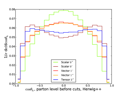
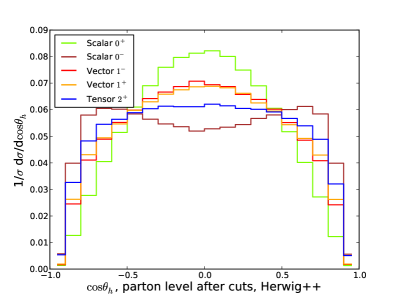
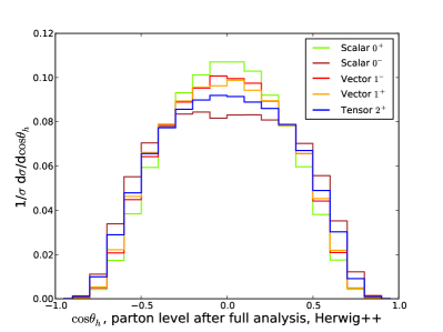
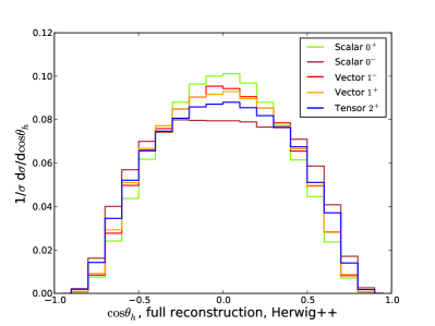
Figure 2: Cosine of the helicity angle $\theta_{h}$, Eq. (1c), calculated from the hadronically decaying $Z$ at different steps of the analysis: inclusive Monte Carlo generation level (top, left), Monte Carlo generation level including selection cuts Eqs. (6)-(8) (top, right), after the full subjet analysis including Monte Carlo-truth information (bottom, left), and after the full analysis (bottom, right).

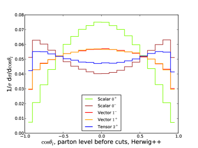
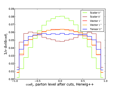
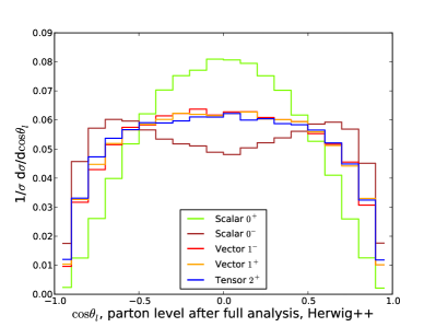
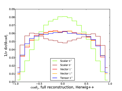
Figure 3: Cosine of the helicity angle $\theta_{\ell}$, Eq. (1c), calculated from the hadronically decaying $Z$ at different steps of the analysis: inclusive Monte Carlo generation level (top, left), Monte Carlo generation level including selection cuts Eqs. (6)-(8) (top, right), after the full subjet analysis including Monte Carlo-truth information (bottom, left), and after the full analysis (bottom, right).

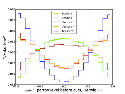
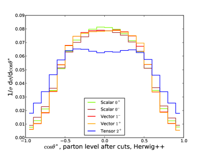
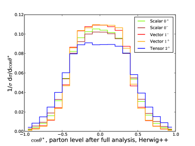
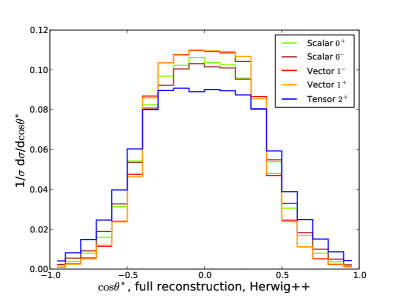
Figure 4: Cosine of the angle $\theta^{\star}$, Eq. (1d), calculated from the hadronically decaying $Z$ at different steps of the analysis: inclusive Monte Carlo generation level (top, left), Monte Carlo generation level including selection cuts Eqs. (6)-(8) (top, right), after the full subjet analysis including Monte Carlo-truth information (bottom, left), and after the full analysis (bottom, right).

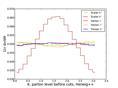
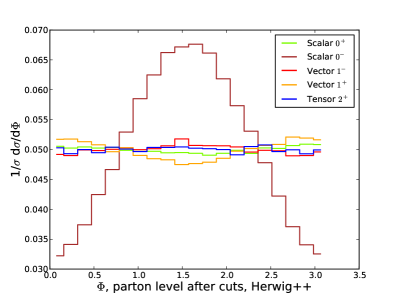
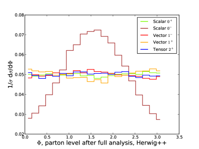
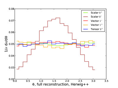
Figure 5: Angle $\Phi$, Eq. (1d), calculated from the hadronically decaying $Z$ at different steps of the analysis: inclusive Monte Carlo generation level (top, left), Monte Carlo generation level including selection cuts Eqs. (6)-(8) (top, right), after the full subjet analysis including Monte Carlo-truth information (bottom, left), and after the full analysis (bottom, right).

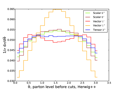
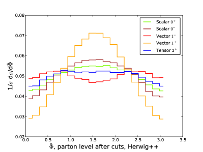
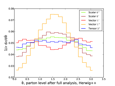
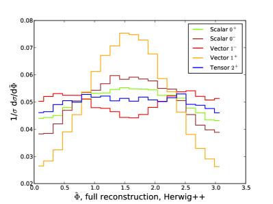
Figure 6: Angle $\tilde{\Phi}$, Eq. (1e), calculated from the hadronically decaying $Z$ at different steps of the analysis: inclusive Monte Carlo generation level (top, left), Monte Carlo generation level including selection cuts Eqs. (6)-(8) (top, right), after the full subjet analysis including Monte Carlo-truth information (bottom, left), and after the full analysis (bottom, right).

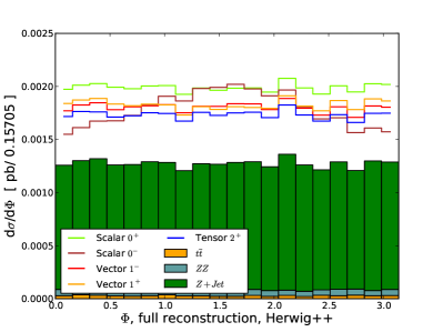
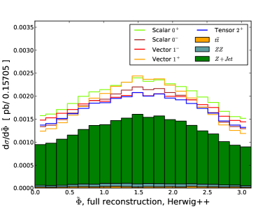
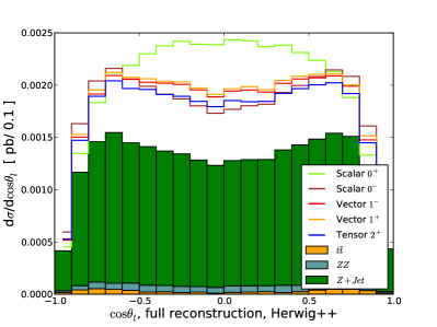
Figure 7: The spin- and $\cal{CP}$-sensitive angles $\Phi$ (top), $\tilde{\Phi}$ (bottom, left) and $\cos\theta_{\ell}$ (bottom, right) including the shape of the backgrounds, simulated with Herwig++.

We include the dominating background processes to our analysis. These are $Z+$jets, $ZZ$, $t\bar{t}$ and $WZ$ production. For the main background $Z+\text{jets}$ the NLO QCD cross section, requiring $p_{T}({\rm{jet}})\geq 100~{}{\rm{GeV}}$, is $33.9$ pb mcfm . The NLO QCD normalization of the $t\bar{t}$ production cross section is $875$ pb Cacciari:2008zb , and for $WZ$ production we find $43.4$ pb mcfm . The NLO QCD $ZZ$ background is $19.0$ pb. For the simulation of the SM Higgs boson we take the NLO gluon-fusion and weak-boson-fusion production mechanism into account and normalize all signals to the inclusive production cross section. We simulate the backgrounds with MadEvent, again employing Pythia 6.4 and Herwig++ for showering, and normalize the distributions to the NLO QCD cross section approximation. For the weak-boson-fusion channels, the NLO QCD corrections are known to be at the percent level for a deep inelastic scattering type of factorization scale choices (see Ref. wbfnlo ; vbfnlo ). For these processes, the electroweak modifications then become important since they turn out to be comparable in size Ciccolini:2007jr . As we perform simulations within an effective electroweak theory approach, and for the smallness of the overall corrections, compared to additional uncertainties presently inherent to showering Alwall:2007fs , we set $\sigma^{\rm{NLO}}/\sigma^{\rm{LO}}=1$ for the weak-boson-fusion contributions. It turns out that the $WZ$ background is negligibly small, and we therefore only focus on the $Z+{\rm{jets}}$, $ZZ$, and $t\bar{t}$ backgrounds in the discussion of our results in Sec. III.

From the fully-simulated Monte Carlo event, we reconstruct the detector calorimeter entries by grouping all final state particles into cells of size $\Delta\eta\times\Delta\phi=0.1\times 0.1$ in the pseudorapidity–azimuthal angle plane, to account for finite resolution of the calorimetry. The resulting cells’ three-momenta are subsequently rescaled such to yield massless cell entries $p^{\mu}p_{\mu}=0$ (see, e.g., Ref. Ball:2007zza ). For the rest of the analysis we discard cells with energy-entries below a calorimeter threshold of $0.5~{}\text{GeV}$.

II.3 Discriminating signal from background

To separate the signal events of Eq. (3) from the background, we perform a fat jet/subjet analysis. The technical layout has been thoroughly discussed in the recent literature, e.g. in Refs. Butterworth:2008iy ; Plehn:2009rk ; Soper:2010xk ; Hackstein:2010wk . We focus on the following on muon production.

Prior to the jet analysis, we therefore require two isolated muons with

$$p_{T}(\mu^{\pm})>15~{}{\rm{GeV}}\quad\hbox{and}\quad|\eta(\mu^{\pm})|<2.5$$ (6)

in the final state, which reconstruct the invariant $Z$ mass up to $10~{}{\rm{GeV}}$,

$$\left[p(\mu^{+})+p(\mu^{-})\right]^{2}=(m_{Z}\pm 10~{}{\rm{GeV}})^{2}\,.$$ (7)

To call a muon isolated we require that $E_{T_{\rm{had}}}<0.1\,E_{T_{\mu^{\pm}}}$ within a cone of $R=0.3$ around the muon. We ask for a “fat jet” with

$$p_{T}(\hbox{fat jet})\geq 150~{}{\rm{GeV}}\quad\hbox{and}\quad|y(\hbox{fat jet})|<2\,,$$ (8)

defined via the inclusive Cambridge-Aachen algorithm Dokshitzer:1997in with resolution parameter $R=1.2$. This particular choice of $R$ guarantees that we pick up the bulk of the $Z$ decay jets since the boosted $Z\rightarrow jj$ decay products’ separation can be estimated to be $\sim 2m_{Z}/p_{T}(Z)$. Throughout, we invoke the algorithms and C++ classes provided by the FastJet framework Cacciari:2005hq .

The hadronic $Z$ reconstruction is performed applying the strategy of Ref. Butterworth:2008iy : For the hardest jet in the event we undo the last stage of clustering, leaving two subjets, which we order with respect to their invariant masses $m_{j_{1}}>m_{j_{2}}$. Provided a significant mass drop for a not too asymmetric splitting,

$$m_{j_{1}}<0.67\,m_{j}\,,\;\;\Delta R_{j_{1}j_{2}}^{2}\text{min}(p_{T,j_{1}}^{2},p_{T,j_{2}}^{2})>0.09\,m_{j}^{2}\,,$$ (9)

where $\Delta R$ denotes the distance in the azimuthal angle–pseudorapidity plane, we consider the jet $j$ to be in the neighborhood of the resonance and terminate the declustering. Otherwise we redefine $j$ to be equal to $j_{1}$ and continue the algorithm until the mass-drop condition is met. In case this does not happen for the considered event, and we discard the event entirely. If the mass-drop condition is met, we proceed with filtering of the fat jet Butterworth:2008iy ; i.e. the constituents of the two subjets which survive the mass drop condition are recombined with higher resolution

$$R_{\text{filt}}=\min\left(0.3\,,{\Delta R_{j_{1}j_{2}}\over 2}\right)\,,$$ (10)

and the three hardest filtered subjets are again required to reproduce the $Z$ mass within $m_{Z}\pm 10~{}\text{GeV}$.

We subsequently reconstruct the Higgs mass from the excess in the $m_{X}^{2}=(p_{Z_{h}}+p_{Z_{\ell}})^{2}$ distribution, i.e. we imagine a situation where the $X$ mass peak has already been established experimentally. This allows us to avoid dealing with the sophisticated details of experimental strategies, which aim to single out the resonance peak from underlying event, pile-up and background distributions by typically including combinations of various statistical methods . A thorough discussion would be beyond the scope of this work. For a considered $X$ mass of $400~{}{\rm{GeV}}$ we include events characterized by reconstructed invariant masses

$$\left[p(\mu^{+})+p(\mu^{-})+p(j_{\alpha})+p(j_{\beta})\right]^{2}=(400\pm 50~{}{\rm{GeV}})^{2}\,.$$ (11)

Further signal-over-background ($S/B$) improvements can be achieved by requiring

$$\Delta R_{ZZ}<3.2$$

and by trimming and pruning Ellis:2009su of the hadronic $Z$ event candidates on the massless cell level of the event Soper:2010xk , as described in detail in Ref. Hackstein:2010wk .

III Results and Discussion

In Figs. 2-7 we show the angles of Eq. (1) after various steps of the analysis have been carried out. We also give a comparison of the full hadron-level result and Monte Carlo truth; i.e. we take into account the shower’s particle information. These plots are the main results of this paper. Comparing the two shower and hadronization approaches of Pythia 6.4 and Herwig++ for the process efficiencies in Table 2, we find substantial discrepancies at intermediate steps of our analysis. After the entire analysis has been carried out this translates into a systematic uncertainty of $\sim 30\%$ of the total cross sections. This is not a too large disagreement as both programs rely on distinct philosophies and approaches, which typically result in sizable deviations when compared for identical Monte Carlo input. The plots in Figs. 2-7 show distributions obtained with Herwig++.

We now turn to the discussion of the angular correlations. It is immediately clear that the chosen selection criteria, Eqs. (6)-(8), do heavily affect the sensitive angular distributions of Eqs. (1). Retaining a signal-over-background ratio of approximately $0.5$, however, does not allow us to relax the $p_{T}$ cut on the fat jet. This cut turns out to be lethal to some of the angular distributions. Referring, e.g., to $\cos\theta^{\star}$, plotted in Fig. 4, we find that our fat jet criteria, Eq. (8), force the distribution into reflecting extremely hard and central decay products. This removes essentially all discriminating features from the differential distribution ${\mathrm{d}}\sigma/{\mathrm{d}}\cos\theta^{\star}$, that show up for $|\cos\theta^{\star}|\gtrsim 0.5$ at the (inclusive) Monte Carlo event generation level. This is also reflected in the distinct acceptance level of the different $J^{\cal{CP}}$ samples, shown in Table 2. Note that, throughout, the fully hadronic distributions are in very good agreement with the Monte Carlo-truth level.

Most of the sensitivity found in the observable $\tilde{\Phi}$ for the signal sample can be carried over to the hadron level. Yet, the angular pattern is known to be sensitive to the $X$’s mass scale, tending to decorrelate for larger $X$ masses (see e.g. Gao:2010qx ).

As already pointed out in Sec.  II, the ambiguity in $\cos\Phi$ smears out the angular correlations quite a lot in Fig. 5. This comes not as too large limitation of the angle’s sensitivity for a ${\cal{CP}}$-odd scalar particle $X$. For $X=0^{-}$, the distribution peaks at $\Phi=\pi/2$ and is also rather symmetrical with respect to $\pi/2$. This leaves us after the subjet analysis with the helicity angles of Eq. (1c) and $\tilde{\Phi}$ as three sensitive angles out of five not taking into account the background distribution.

Crucial to obtaining angular correlations after all, is the analysis’ capability to reconstruct both of the $Z$ rest frames (and from them the $X$ rest frame). This is already clear from the angles’ definition in Eq. (1), and, again, this is not an experimental problem considering the purely leptonic channels. For the angles $\Phi$ and $\theta^{\star}$ decorrelate (with the exception of $0^{-}$) due to the selection criteria, a bad rest frame reconstruction would not be visible in these observables immediately. This is very different if we turn to the helicity angles. Quite obviously, given a good hadronically decaying $Z$ rest frame reconstruction, we can apply the identical leptonic helicity angle as invoked for the measurement in $X\rightarrow ZZ\rightarrow 4\ell$; we have referred to this angle as $\theta_{\ell}$, previously. The only difference compared to the purely leptonic analysis is that we consult a partly hadronic system to construct the reference system, in which the leptonic helicity angle $\theta_{\ell}$ is defined.

Indeed, the subjet analysis described in Sec. II.3 is capable of giving a very good reconstruction of the hadronically decaying $Z$ boson rest frame, while sufficiently reducing the backgrounds. This allows to carry over most of the central sensitivity of the angular distributions in Fig. 3 to the fully simulated final state. However, the hadronically-defined helicity angle, displayed in Fig. 2, also suffers badly from the subjet analysis. Note that the bulk of the modifications of $\cos\theta_{h}$ do not arise from our restrictive selection criterion Eq. (8), but from symmetry requirements among the subjets in the mass-drop procedure. Thus, the subjets which provide a significant mass drop with respect to Eq. (9) are biased towards $\theta_{h}\simeq 90^{\circ}$.

A remaining key question that needs to be addressed is whether the potentially sensitive angles $\theta_{\ell},\Phi$, and $\tilde{\Phi}$ exhibit visible spin- and ${\cal{CP}}$-dependent deviations when the background distribution is taken into account. We show these angles including the backgrounds in Fig. 7. The backgrounds’ $\tilde{\Phi}$ distribution largely mimics the $1^{+}$ shape under the subjet analysis’ conditions, so we cannot claim sensitivity unless the backgrounds distribution is very well known. This also accounts for the $\Phi$ distribution in a milder form. While here the background is flat to good approximation, $S/B$ (see Table 2) limits the sensitivity to the shape deviations, which are ameliorated due to the different signal efficiencies. However, the distribution remains sensitive to $X=0^{-}$ shape. $pp\rightarrow X\rightarrow\mu^{+}\mu^{-}jj$ remains sensitive to the ${\cal{CP}}$ quantum number of a scalar particle $X$ in the $\cos\theta_{\ell}$ distribution, which is opposite in shape compared to the background distribution.

We have only considered an $X$ mass $m_{X}=400~{}{\rm{GeV}}$, a choice which is quite close to the lower limit of the mass range, where the boosted analysis is applicable. Some remarks concerning our analysis for different $X$ masses and widths are due. The boost requirements and the centrally required selection cuts do affect the angular distributions in a $X$ mass-independent manner. The remaining angles are then qualitatively determined by the goodness of reconstruction, which becomes increasingly better for heavier $X$ masses, keeping the width fixed.

In case of the SM Higgs boson, the width is proportional to $m_{H}^{3}$ due to the enhanced branching of the Higgs to longitudinally-polarized $Z$s. With the resonance becoming width-dominated, our mass reconstruction still remains sufficiently effective; $S/B$, however, increasingly worsens. For these mass ranges, the analysis is sensitive to the experimental methods that recover the resonance excess. Additionally, from a theoretical perspective, there are various models known in the literature where a heavy resonance becomes utterly narrow or exceedingly broad (see, e.g. Birkedal:2004au ; Bagger:1995mk for discussions of the resulting phenomenology). The former yields, depending on the (non-SM) production cross section, a better mass reconstruction, while the latter case is again strongly limited by $S/B$; cf. Fig. 7. For any of these EWSB realizations, our methods should be modified accordingly, taking into account all realistic experimental algorithms, techniques, and uncertainties as well as all model-dependent parameters.

IV Summary and Conclusions

The discovery of a singly produced new state at the LHC, and methods to determine its additional quantum numbers, remains an active field of particle physics phenomenology research. The availability of tools to simulate events at a crucial level of realism and precision has put the phenomenology community into a position that allows a more transparent view onto the complicated particle dynamics at high-energy hadron colliders than ever.

In this paper we have explored the performance of new jet techniques when applied to the analysis of spin- and ${\cal{CP}}$-sensitive distributions of a newly discovered resonance, which resembles the SM in the overall rate in $pp\rightarrow\mu^{+}\mu^{-}jj$. We have performed a detailed investigation of the angular correlations and have worked out the approach-specific limitations, resulting from the boosted and central kinematical configurations. It is self-evident that a QCD-dominated final state cannot compete with a leptonic final state in terms of signal purity, higher order and shower uncertainties, per se. These uncertainties are inherent to any current discussion related to jet physics. Nonetheless, we have shown that potential “no-go theorems” following from huge underlying event and QCD background rates for $pp\rightarrow X\rightarrow ZZ\rightarrow\ell^{+}\ell^{-}jj$ can be sufficiently ameliorated to yield an overall sensitivity to the ${\cal{CP}}$ property of a singly produced scalar resonance. Straightforwardly applying the described analysis strategy to vectorial and tensorial resonances does not yield reliable shape deviations when the backgrounds’ distribution is taken into account. Given that the cross section of the semihadronic decay channel is approximately 10 times larger compared to $X\rightarrow 4\ell$, the performed subjet analysis qualifies to at least supplement measurements of the purely leptonic decay channels.

A question we have not addressed in this paper is the potential application of the presented strategy to signatures, which do not resemble the SM at all. Electroweak symmetry breaking by strong interactions is likely to yield a large rate of longitudinally polarized electroweak bosons due to modified $XZZ$ and $X\bar{q}q$ couplings Chanowitz:1985hj ; silh . Measuring the fraction of longitudinal polarizations, which can be inferred from the $Z$’s decay products’ angular correlation as proposed recently in Ref. Han:2009em , should benefit from the methods we have investigated in this paper. This is in particular true for new composite operators, such as a modification of the Higgs kinetic term silh , inducing asymmetric angular decay distributions of the leptons. In addition, our analysis is also applicable to the investigation of isovectorial resonances (see, e.g., Ref. Bagger:1995mk ) in $pp\rightarrow WZ$, with the $W$ decaying to hadrons, and $Z\rightarrow\mu^{+}\mu^{-}$. We leave a more thorough investigation of these directions to future work.

Acknowledgments — We thank Tilman Plehn for many discussions and valuable comments on the manuscript. This work was supported in part by the US Department of Energy under Contract No. DE-FG02-96ER40969. C.H. is supported by the Graduiertenkolleg “High Energy Particle and Particle Astrophysics”. Parts of the numerical calculations presented in this paper have been performed using the Heidelberg/Mannheim and Karlsruhe high performance clusters of the bwGRiD (http://www.bw-grid.de), member of the German D-Grid initiative, funded by the Ministry for Education and Research (Bundesministerium für Bildung und Forschung) and the Ministry for Science, Research and Arts Baden-Wuerttemberg (Ministerium für Wissenschaft, Forschung und Kunst Baden-Württemberg). C.H. thanks M. Soysal for the support using the Karlsruhe cluster.

References

- (1) J. M. Cornwall, D. N. Levin and G. Tiktopoulos, Phys. Rev. Lett. 30 (1973) 1268 [Erratum-ibid. 31 (1973) 572],
- (2) G. Aad et al. [ATLAS Collaboration], JINST 3 (2008) S08003.
- (3) G. L. Bayatian et al. [CMS Collaboration], J. Phys. G 34 (2007) 995.
- (4) C. P. Buszello, I. Fleck, P. Marquard and J. J. van der Bij, Eur. Phys. J. C 32 (2004) 209.
- (5) C. P. Buszello, P. Marquard and J. J. van der Bij, arXiv:hep-ph/0406181.
- (6) S. Y. Choi, D. J. . Miller, M. M. Muhlleitner and P. M. Zerwas, Phys. Lett. B 553 (2003) 61, R. M. Godbole, D. J. . Miller and M. M. Muhlleitner, JHEP 0712 (2007) 031, P. S. Bhupal Dev, A. Djouadi, R. M. Godbole, M. M. Muhlleitner and S. D. Rindani, Phys. Rev. Lett. 100 (2008) 051801.
- (7) Y. Gao, A. V. Gritsan, Z. Guo, K. Melnikov, M. Schulze and N. V. Tran, Phys. Rev. D 81, 075022 (2010).
- (8) A. De Rujula, J. Lykken, M. Pierini, C. Rogan and M. Spiropulu, Phys. Rev. D 82 (2010) 013003.
- (9) J.-C. Chollet et al., ATLAS note PHYS-NO-17 (1992), L. Poggioli, ATLAS Note PHYS-NO-066 (1995);, D. Denegri, R. Kinnunen and G. Roullet, CMS-TN/93-101 (1993), I. Iashvili R. Kinnunen, A. Nikitenko and D. Denegri, CMS TN/95-076, D. Bomestar et al., Note CMS TN-1995/018, C. Charlot, A. Nikitenko and I. Puljak, CMS TN/95-101, G. Martinez, E. Gross, G. Mikenberg and L. Zivkovic, ATLAS Note ATL-PHYS-2003-001 (2003).
- (10) J. M. Butterworth, A. R. Davison, M. Rubin and G. P. Salam, Phys. Rev. Lett. 100 (2008) 242001.
- (11) T. Plehn, G. P. Salam and M. Spannowsky, Phys. Rev. Lett. 104 (2010) 111801.
- (12) D. E. Soper and M. Spannowsky, JHEP 1008 (2010) 029.
- (13) M. H. Seymour, Z. Phys. C 62, 127 (1994).
- (14) G. Brooijmans, ATL-PHYS-CONF-2008-008 and ATL-COM-PHYS-2008-001, Feb. 2008, J. Thaler and L. T. Wang, JHEP 0807, 092 (2008), D. E. Kaplan, K. Rehermann, M. D. Schwartz and B. Tweedie, Phys. Rev. Lett. 101, 142001 (2008), L. G. Almeida, S. J. Lee, G. Perez, G. Sterman, I. Sung and J. Virzi, Phys. Rev. D 79, 074017 (2009), S. Chekanov and J. Proudfoot, Phys. Rev. D 81, 114038 (2010), T. Plehn, M. Spannowsky, M. Takeuchi and D. Zerwas, arXiv:1006.2833 [hep-ph], ATLAS Collaboration ATL-PHYS-PUB-2009-081, CMS Collaboration CMS-PAS-JME-09-001, G. D. Kribs, A. Martin, T. S. Roy and M. Spannowsky, Phys. Rev. D 81 (2010) 111501, G. D. Kribs, A. Martin, T. S. Roy and M. Spannowsky, arXiv:1006.1656 [hep-ph], C. R. Chen, M. M. Nojiri and W. Sreethawong, arXiv:1006.1151 [hep-ph], A. Falkowski, D. Krohn, L. T. Wang, J. Shelton and A. Thalapillil, arXiv:1006.1650 [hep-ph], L. G. Almeida, S. J. Lee, G. Perez, G. Sterman and I. Sung, arXiv:1006.2035 [hep-ph], K. Rehermann and B. Tweedie, arXiv:1007.2221 [hep-ph], S. Chekanov, C. Levy, J. Proudfoot and R. Yoshida, arXiv:1009.2749 [hep-ph].
- (15) C. Hackstein and M. Spannowsky, arXiv:1008.2202 [hep-ph].
- (16) N. D. Christensen, T. Han and Y. Li, Phys. Lett. B 693 (2010) 28.
- (17) M. Duhrssen, S. Heinemeyer, H. Logan, D. Rainwater, G. Weiglein and D. Zeppenfeld, Phys. Rev. D 70 (2004) 113009, R. Lafaye, T. Plehn, M. Rauch, D. Zerwas and M. Duhrssen, JHEP 0908 (2009) 009, S. Bock, R. Lafaye, T. Plehn, M. Rauch, D. Zerwas and P. M. Zerwas, Phys. Lett. B 694 (2010) 44.
- (18) A. Birkedal, K. Matchev and M. Perelstein, Phys. Rev. Lett. 94 (2005) 191803, H. J. He et al., Phys. Rev. D 78 (2008) 031701, C. Englert, B. Jager and D. Zeppenfeld, JHEP 0903 (2009) 060.
- (19) M. S. Chanowitz and M. K. Gaillard, Nucl. Phys. B 261 (1985) 379,
- (20) G. F. Giudice, C. Grojean, A. Pomarol and R. Rattazzi, JHEP 0706 (2007) 045, J. R. Espinosa, C. Grojean and M. Muhlleitner, JHEP 1005 (2010) 065.
- (21) M. J. Strassler and K. M. Zurek, Phys. Lett. B 651 (2007) 374.
- (22) N. Cabibbo and A. Maksymowicz, Phys. Rev. 137, B438 (1965) [Erratum-ibid. 168, 1926 (1968)].
- (23) A. Bredenstein, A. Denner, S. Dittmaier and M. M. Weber, Phys. Rev. D 74 (2006) 013004.
- (24) Q. H. Cao, C. B. Jackson, W. Y. Keung, I. Low and J. Shu, Phys. Rev. D 81 (2010) 015010.
- (25) T. L. Trueman, Phys. Rev. D 18 (1978) 3423, J. R. Dell’Aquila and C. A. Nelson, Phys. Rev. D 33 (1986) 80.
- (26) J. C. Collins and D. E. Soper, Phys. Rev. D 16 (1977) 2219.
- (27) G. L. Bayatian et al. [CMS Collaboration], CMS-TDR-008-1.
- (28) T. Plehn, D. L. Rainwater and D. Zeppenfeld, Phys. Rev. Lett. 88 (2002) 051801, T. Figy and D. Zeppenfeld, Phys. Lett. B 591 (2004) 297, V. Hankele, G. Klamke, D. Zeppenfeld and T. Figy, Phys. Rev. D 74 (2006) 095001, G. Klamke and D. Zeppenfeld, JHEP 0704 (2007) 052.
- (29) J. Alwall et al., JHEP 0709 (2007) 028.
- (30) K. Hagiwara and D. Zeppenfeld, Nucl. Phys. B 313 (1989) 560. H. Murayama, I. Watanabe and K. Hagiwara, KEK-Report 91-11, 1992.
- (31) K. Hagiwara, J. Kanzaki, Q. Li and K. Mawatari, Eur. Phys. J. C 56 (2008) 435.
- (32) A. Djouadi, Phys. Rept. 457 (2008) 1, V. Buescher and K. Jakobs, Int. J. Mod. Phys. A 20, 2523 (2005).
- (33) W. H. Furry, Phys. Rev., 51, 125 (1937).
- (34) C. N. Yang, Phys. Rev. 77 (1950) 242.
- (35) W. Buchmuller and D. Wyler, Nucl. Phys. B 268 (1986) 621, K. Hagiwara, R. D. Peccei, D. Zeppenfeld and K. Hikasa, Nucl. Phys. B 282 (1987) 253.
- (36) W. Y. Keung, I. Low and J. Shu, Phys. Rev. Lett. 101 (2008) 091802.
- (37) V. M. Abazov et al. [The D Collaboration], Phys. Rev. Lett. 104 (2010) 241802.
- (38) M. Spira, Nucl. Instrum. Meth. A 389, 357 (1997).
- (39) K. Arnold et al., Comput. Phys. Commun. 180, 1661 (2009).
- (40) M. Bahr et al., Eur. Phys. J. C 58 (2008) 639.
- (41) T. Sjostrand, S. Mrenna and P. Z. Skands, JHEP 0605, 026 (2006).
- (42) J. M. Campbell and R. K. Ellis, Phys. Rev. D 60, 113006 (1999), J. M. Campbell and R. K. Ellis, arXiv:1007.3492 [hep-ph]; http://mcfm.fnal.gov.
- (43) M. Cacciari, S. Frixione, M. L. Mangano, P. Nason and G. Ridolfi, JHEP 0809, 127 (2008).
- (44) T. Figy, C. Oleari and D. Zeppenfeld, Phys. Rev. D 68, 073005 (2003), B. Jager, C. Oleari and D. Zeppenfeld, Phys. Rev. D 73, 113006 (2006), G. Bozzi, B. Jager, C. Oleari and D. Zeppenfeld, Phys. Rev. D 75 (2007) 073004, A. Bredenstein, K. Hagiwara and B. Jager, Phys. Rev. D 77 (2008) 073004,
- (45) M. Ciccolini, A. Denner and S. Dittmaier, Phys. Rev. Lett. 99 (2007) 161803, M. Ciccolini, A. Denner and S. Dittmaier, Phys. Rev. Lett. 99, 161803 (2007),
- (46) J. Alwall et al., Eur. Phys. J. C 53 (2008) 473.
- (47) Y. L. Dokshitzer, G. D. Leder, S. Moretti and B. R. Webber, JHEP 9708, 001 (1997), M. Wobisch and T. Wengler, arXiv:hep-ph/9907280.
- (48) M. Cacciari and G. P. Salam, Phys. Lett. B 641, 57 (2006). M. Cacciari, G. P. Salam and G. Soyez, http://fastjet.fr.
- (49) S. D. Ellis, C. K. Vermilion and J. R. Walsh, Phys. Rev. D 80, 051501 (2009), S. D. Ellis, C. K. Vermilion and J. R. Walsh, Phys. Rev. D 81 (2010) 094023, D. Krohn, J. Thaler and L. T. Wang, JHEP 1002, 084 (2010).
- (50) J. Bagger et al., Phys. Rev. D 49 (1994) 1246, J. Bagger et al., Phys. Rev. D 52 (1995) 3878, C. Englert, B. Jager, M. Worek and D. Zeppenfeld, Phys. Rev. D 80 (2009) 035027.
- (51) T. Han, D. Krohn, L. T. Wang and W. Zhu, JHEP 1003 (2010) 082.