Inelastic scattering of atoms in a double well

Abstract

We study a mixture of two light spin-1/2 fermionic atoms and two heavy atoms in a double well potential. Inelastic scattering processes between both atomic species excite the heavy atoms and renormalize the tunneling rate and the interaction of the light atoms (polaron effect). The effective interaction of the light atoms changes its sign and becomes attractive for strong inelastic scattering. This is accompanied by a crossing of the energy levels from singly occupied sites at weak inelastic scattering to a doubly occupied and an empty site for stronger inelastic scattering. We are able to identify the polaron effect and the level crossing in the quantum dynamics.

I Introduction

Ultracold bosonic and fermionic atomic gases in optical lattices can be used as a toolkit for the investigation of fundamental condensed matter physics models lewen07 . Recent experimental work opened a field to study quantum states in optical lattices, such as superfluid and Mott states greiner02 ; bloch05 , where the interparticle interaction can be controlled by a magnetic field via a Feshbach resonance feshb . Spin-dependent effects ketterle03 ; mandel03 ; schmaljohann04 ; kohl05 ; partridge06 , frustrated spin systems lewenstein06 , the formation of dimers from fermionic atoms hulet03 ; uys05 , and mixtures of two atomic species stan04 ; esslinger06 ; sengstock06 provide opportunities for creating and studying even more complex quantum states.

The optical lattices are robust and free of phonons. On the other hand, the electron-phonon interaction in a solid leads to a rich physics. It is important for superconductivity, the Peierls instability, polaron effects and many other phenomena. With more progress in the atomic and laser physics, the coupling of ultracold atoms in an optical lattice to bosonic degrees of freedom may be achieved and thus can mimic the dynamics of electrons in the presence of phonons. Recently, ultracold atoms confined to an optical resonator were proposed to study the effect of coupling between the atoms and the photons field, which leads to an effective Hubbard Hamiltonian with long-range interaction Ritsch05 and to an interesting phase diagram lewen06 . Bose-Fermi mixtures can also provide an insight into the role of bosons in the dynamics of fermions, where the condensed bosons lead to fermionic pairing wang06 and charge density waves of fermions hofst08 . An interesting example of the latter are dimer states. They have been discussed in solid-state systems rokhsar88 , in the Holstein-Hubbard model ziegler08 and recently also for an ultracold Bose gas with ring exchange xu06 .

More recently, ultracold gases were employed to study the dynamics of quantum states, including the “collapse and revival” behavior greiner02b . Here it is important to distinguish between small systems with a few atoms and many-body systems with a large number of atoms lewen07 . For instance, it was observed experimentally that in a small system with two spin-1/2 atoms the spin dynamics and the particle dynamics are completely separated, similar to the spin-charge separation in one-dimensional systems bloch07 ; bloch08 . Another example for a restricted dynamics in small atomic systems are entangled squeezed states in a Bose-Einstein condensate, whose atoms are distributed over a small number of lattice sites ober08 . Both observations indicate that the dynamics of small atomic systems can be restricted to a subspace of the entire Hilbert space available for the model Hamiltonian. This can also mean that the system never reaches the groundstate of the Hamiltonian if it was prepared in an excited state, reflecting the fact that the initial state has no overlap with the groundstate. For two spin-1/2 atoms in a double well, described by a Hubbard model, this is a direct consequence of the fact that the eigenstates do not mix pairs of singly occupied sites with pairs of empty and doubly occupied sites ziegler09 . On the other hand, mixing of these states in a macroscopic system, enforced by inelastic scattering with other atoms, can lead to a first-order quantum phase transition from singly occupied sites to doubly occupied sites. This was observed in a mixture of light and heavy atoms, where the latter are in a Mott state ziegler08 . This case can be described by a Bose-Fermi model that is known in solid-state physics as the Holstein-Hubbard (HH) model alexandrov95 . Adjusting physical parameters, such as the optical-lattice parameters (frequency and amplitude of the Laser field) and the fermion-fermion interaction through a Feshbach resonance, enables us to prepare such a system not only in the ground state but also in its excited states and to study its dynamics. Although in a small system there is no phase transition for the ground state, dynamical properties of excited states can change qualitatively due to inelastic scattering described by the HH model. Among other effects, there is renormalization of the tunneling rate, known as the polaron effect, which was recently also discussed for an ultracold Bose gas tempere09 .

Our interest is to study the effect of inelastic scattering of two spin-1/2 fermionic atoms in a double-well potential with repulsive Hubbard interaction and an additional scattering with a heavy atom in each potential well. Each of the heavy atoms have a harmonic oscillator spectrum and can exchange energy with the tunneling spin-1/2 atoms.

In this paper, we study a double well potential filled with heavy (bosonic or fermionic) atoms (HA) (e.g. ⁸⁷Rb or ⁴⁰K), one at each well (see Fig. 1). A double-well potential can be realized by superimposing two periodic potentials with different periodicity and the dynamics of one or two atoms can be easily studied.

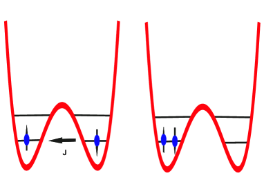
Figure 1: Two LFA in a double well potential with one HA in each well. The HA are harmonic oscillators and are represented by horizontal lines (energy levels). The LFA can tunnel from one well to the other one. The wells can be singly occupied (left panel) or one well can be doubly occupied and the other one empty (right panel).

The tunneling of these HA is neglected since the potential barrier between the wells is sufficiently high. Excitations are only due to collisions with other atoms. For this purpose two light fermionic atoms (LFA) (e.g. ⁶Li), prepared in two hyperfine states denoted as $|\!\uparrow\rangle$, $|\downarrow\rangle$, are added to the system. These atoms can tunnel because of their low mass and scatter by the HA. It is assumed that the HA experience a harmonic potential of a well, at least at low energies. Then their excitations are harmonic-oscillator states. During the scattering process the HA can also transfer energy to the LFA. Moreover, the light fermions experience local (on-site) repulsion.

The paper is organized as follows. The Holstein-Hubbard model is introduced and discussed in Sect. II. In Sect. III we introduce a restricted model with at most one phonon excitation per well. Then in Sect. IV the effective Hamiltonian of the unrestricted Holstein-Hubbard model is defined, its spectral properties are studied and compared with those of the restricted model of Sect. III. Based on this effective Hamiltonian we study the dynamics of the quantum states in a double well, the spectral density and the spin imbalance in Sect. V.

II Holstein-Hubbard Model

The atomic mixture of LFA and HA can be well described by the Holstein-Hubbard model alexandrov95 :

$$H=-J\sum_{<{\bf j},{\bf j}^{\prime}>}\sum_{\sigma=\uparrow,\downarrow}c_{{\bf j}\sigma}^{\dagger}c_{{\bf j}^{\prime}\sigma}^{\phantom{ab}}+h.c.+\sum_{{\bf j}}\Big{[}\omega_{0}b_{\bf j}^{\dagger}b_{\bf j}+g(b_{\bf j}^{\dagger}+b_{\bf j})(n_{{\bf j}\uparrow}+n_{{\bf j}\downarrow})+Un_{{\bf j}\uparrow}n_{{\bf j}\downarrow}\Big{]}\hskip 5.69046pt.$$ (1)

The first term describes the tunneling of LFA with spin $\sigma$ ($=\uparrow,\downarrow$) between nearest-neighbor wells. These are defined by fermionic creation and annihilation operators $c_{{\bf j}\sigma}^{\dagger}$ and $c_{{\bf j}\sigma}$, respectively. The HA form a Mott state and are presented as harmonic oscillators at each well with eigenfrequency $\omega_{0}$, assuming that a HA in one well is excited independently of the HA in the other well. Thus they can be considered as local phonons and are described by the bosonic creation and annihilation operators $b_{\bf j}^{\dagger}$ and $b_{\bf j}$. The phonons couple to the light atoms with strength $g\sim\langle e|\hat{V}|f\rangle$, where $\hat{V}$ is the interaction between LFA and HA, $|f\rangle$ denotes the ground state of a HA, while $|e\rangle$ denotes its first excited state. The fourth term describes the interaction between two LFA at the same well, where $U$ is a local repulsive interaction between the LFA

This lattice model describes the quantum phase transition in a half-filled system from singly occupied lattice wells (Néel state) to a mixture of doubly occupied and empty wells (dimer state). Now we restrict the lattice model to the two sites of the double well potential, choosing the coordinates $j=1,2$ for the wells. Ignoring the tunneling of the LFA and applying a unitary transformation to the remaining part of the Hamiltonian we can decouple fermionic and bosonic degrees of freedom and get the transformed local Hamiltonian ziegler08

$$H_{\gamma}=\sum_{{\bf j}=1,2}\left[\omega_{0}b^{\dagger}_{\bf j}b_{\bf j}+\gamma n_{{\bf j}\uparrow}n_{{\bf j}\downarrow}-{g^{2}\over\omega_{0}}(n_{{\bf j}\uparrow}+n_{{\bf j}\downarrow})\right]\hskip 5.69046pt$$ (2)

with $\gamma=U-2g^{2}/\omega_{0}$ is the effective Hubbard coupling. For a system with two fermions the ground state energy of $H_{\gamma}$ is given by

$$E_{0}=\epsilon-\gamma j\hskip 5.69046pt,$$ (3)

with $\epsilon=U-4g^{2}/\omega_{0}$ and $2j$ is the number of singly occupied wells. The coupling $\gamma$ controls two different regimes: for $\gamma>0$, the ground state has two singly occupied wells ($j=1$) and energy $-2g^{2}/\omega_{0}$, while for $\gamma<0$, there are one doubly occupied well and one empty well ($j=0$) and the energy is $\epsilon$. Thus at $\gamma=0$ there is a transition, where the system changes from two singly occupied wells to a doubly occupied well and an empty well. Moreover, both states are degenerate even for $\gamma\neq 0$ because the local Hamiltonian $H_{\gamma}$ does not determine how the spins, and the empty and doubly occupied wells are distributed in the double-well potential. Tunneling in the Hamiltonian $H$ lifts these degeneracies alexandrov95 .

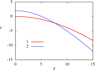
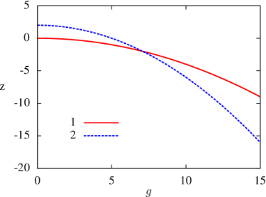
Figure 2: Model without tunneling ($J=0$): Four degenerate eigenvalues of the two-sites problem with at most one phonon excitation (left panel) and the four lowest poles of the resolvent of Eq. (4) with the effective Hamiltonian $H_{\rm eff}$ in Eq. (5) (right panel) for $U=2$ and $\omega_{0}=50$. Curve 1 (curve 2) represent levels with two singly (one empty and one doubly) occupied wells. Left panel: The two curves cross at $g\approx 7.6$. The energy of the ground state has a cusp, but it does not coincide with the exact ground state for $J=0$ given in Eq. (3). Right panel: The two curves cross at the smaller value $g=5\sqrt{2}\approx 7.07$.

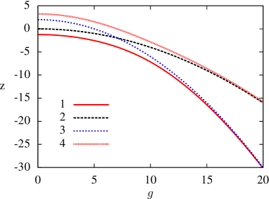
Figure 3: Model with tunneling ($J=1$): Four eigenvalues of the two-sites problem with at most one phonon excitation (left panel) and the four lowest poles of the resolvent of Eq. (4) with the effective Hamiltonian $H_{\rm eff}$ of Eq. (5) (right panel) for $U=2$ and $\omega_{0}=50$. Left panel: The curve 2 and the curve 3 cross at $g\approx 7.6$. For very large values of coupling $g$ the distances between curve 1 and curve 3, as well as between curve 2 and curve 4, remain nonzero. Right panel: The curve 2 and the curve 3 cross at $g\approx 7.1$. For very large values of coupling $g$ the distances between curve 1 and curve 3, as well as between curve 2 and curve 4, vanish as $\sim\tau^{2}/|\gamma|$. This is due to the polaron effect, which accounts for rescaling of the single fermion tunneling $J\rightarrow\tau=Je^{-g^{2}/\omega_{0}^{2}}$.

III Double well with at most one phonon excitation per well

Even for a double well with two fermions the Hilbert space of the Hamiltonian in Eq. (1) has infinite dimensions due to the phonon excitations. For nonzero tunneling rate $J$ this becomes a difficult problem. However, to study qualititatively the effect of inelastic scattering we can restrict the phonon excitations. The simplest case is a model in which each of the localized atoms is a two-level system, similar to the Jaynes-Cummings model in quantum optics jaynes63 . For $J=0$ the four lowest eigenvalues are degenerated in pairs, as shown in the left panel of Fig. 2. The ground state has a cusp, but the latter does not coincide with the exact ground state for $J=0$ given in Eq. (3). A nonzero tunneling rate $J$ lifts the degeneracy and all four eigenvalues are distinct now (cf. left panel of Fig. 3). We notice that for large values of $g$ the curves do not merge (i.e., the distances between the first and the third, and the second and fourth curves, respectively, remain nonzero).

IV Effective Hamiltonian for many phonon excitations

Now we consider the full Holstein-Hubbard Hamiltonian in Eq. (1) and treat its spectral properties in an approximative manner. The main idea is to study the evolution of the quantum system $|\Psi_{t}\rangle=e^{-itH}|\Psi_{0}\rangle$, beginning with the initial state $|\Psi_{0}\rangle$. The evolution is a walk through the entire Hilbert space that is accessible for the Hamiltonian. The Recursive Projective method (RPM) organizes this walk by projecting iteratively on a sequence of subspaces. The main advantage of this method is that the walk visits each subspace only once ziegler03 ; ziegler06 ; ziegler09 . The approximation method within the RPM consists of ignoring some part of the Hilbert space that contributes with a low probability to the walk and leads to an effective Hamiltonian. Details of the application of the RPM to the Holstein-Hubbard Hamiltonian can be found in Ref. ziegler08 . In the following we start from the effective Hamiltonian that was derived in Ref. ziegler08 , to study the dynamics of the LFA in the double-well potential. The advantage of this method is that it enables us to study the effect of finite tunneling of the LFA as well as arbitrary number of phonon excitations.

In order to derive an effective Hamiltonian, we project the full Hilbert space of the Hamiltonian in Eq. (1) onto the Hilbert space spanned by the four Fock states $|\!\uparrow,\downarrow\rangle$ , $|\downarrow,\uparrow\rangle$ , $|0,\uparrow\downarrow\rangle$ and $|\!\uparrow\downarrow,0\rangle$ with a projector $P_{0}$, such that the resolvent of the projected Hamiltonian is given by

$$G_{0}(z)=P_{0}(z-H)^{-1}P_{0}=\bigl{(}z-H_{\rm eff}(z)\bigl{)}^{-1}_{0}\hskip 5.69046pt.$$ (4)

The effective Hamiltonian for the double well can be evaluated recursively by the RPM. Under the assumption that the tunneling rate of LFA $J$ is small compared to the other parameters of the system (e.g. $J\ll\omega_{0}$, $J\ll U$ and $J\ll g$) the recursion relation can be truncated, which gives ziegler08

$$H_{\rm eff}(z)\approx\sum_{\sigma,\sigma^{\prime}=\uparrow,\downarrow}\left[-\tau c^{\dagger}_{1\sigma}c_{2\sigma}+K_{1}(z)c_{1\sigma}^{\dagger}c_{2\sigma}c_{2\sigma^{\prime}}^{\dagger}c_{1\sigma^{\prime}}\right.\left.+K_{2}(z)c_{1\sigma}^{\dagger}c_{2\sigma}c_{1\sigma^{\prime}}^{\dagger}c_{2\sigma^{\prime}}+h.c.+\frac{\gamma}{2}(n_{1\sigma}n_{1\sigma^{\prime}}+n_{2\sigma}n_{2\sigma^{\prime}})\right],$$ (5)

where the indices 1 and 2 represent the left and right sites of the double well, respectively. This Hamiltonian describes three different tunneling processes, namely the tunneling of single fermions with rate $\tau$ (first term), the exchange of spins with rate $K_{1}(z)$ (second term), the tunneling of fermionic pairs with rate $K_{2}(z)$ (third term) and the on-site interaction between fermions with strength $\gamma$ (fourth term). The tunneling rate $J$ of single fermions in Eq. (1) is now renormalized as

$$\tau=e^{-g^{2}/\omega_{0}^{2}}J\ ,$$ (6)

which is the well-known polaron effect alexandrov95 . The spin-exchange parameter $K_{1}$ and the pair tunneling parameter $K_{2}$ are given by the expressions ziegler08

$$K_{1}(z)~{}=~{}2\tau^{2}\sum_{m=1}^{\infty}\frac{1}{m!}\frac{\bigl{(}2g^{2}/\omega_{0}^{2}\bigr{)}^{m}}{z\,-\,2\epsilon\,+\,2\gamma\,-\,\omega_{0}m}$$ (7)

and

$$K_{2}(z)~{}=~{}2\tau^{2}\sum_{m=1}^{\infty}\frac{1}{m!}\frac{\bigl{(}-2g^{2}/\omega_{0}^{2}\bigr{)}^{m}}{z\,-\,2\epsilon\,-\,\omega_{0}m}.$$ (8)

In order to avoid the singularities of the coefficients $K_{1}$ and $K_{2}$, we assume that $\omega_{0}\gg U,g$, which is valid for a deep and tight double-well potential.

The energy levels of the system is given by the poles of Eq. (4). Thus the variable $z$ is fixed by solving the equation

$$\det[z-H_{\rm eff}(z)]=0.$$ (9)

To solve this equation we first diagonalize the $4\times 4$ effective Hamiltonian $H_{\rm eff}$ for a fixed parameter $z$ and find its eigenvalues $\lambda_{j}(z)$ ($j=1,...,4$). Then we solve $z=\lambda_{j}(z)$ for each of the four eigenvalues $\lambda_{j}(z)$ to determine the poles of the resolvent in Eq. (4). An eigenstate $|E\rangle$ (with $H_{\rm eff}|E\rangle=E|E\rangle$) can be written as a linear combination of the four Fock states as

$$|E\rangle=a_{1}(z)|\!\uparrow,\downarrow\rangle+a_{2}(z)|\!\downarrow,\uparrow\rangle+a_{3}(z)|0,\uparrow\downarrow\rangle+a_{4}(z)|\!\uparrow\downarrow,0\rangle\hskip 5.69046pt,$$ (10)

where the coefficients $a_{j}(z)$ run over all possible poles $z$. In this Fock-state basis the Hamiltonian in Eq. (5) reads

$${\hat{H}}_{\rm eff}(z)=\left(\begin{array}[]{cccc}K_{1}+\epsilon-\gamma&-K_{1}&-\tau&-\tau\\ -K_{1}&K_{1}+\epsilon-\gamma&\tau&\tau\\ -\tau&\tau&K_{1}+\epsilon&K_{2}\\ -\tau&\tau&K_{2}&K_{1}+\epsilon\end{array}\right)\hskip 5.69046pt,$$ (11)

whose eigenvalues and the coefficients of the corresponding (non-normalized) eigenvectors in the form of Eq. (10) are for doubly occupied lattice sites

$$\lambda_{1}(z)=K_{1}(z)-K_{2}(z)+\epsilon:\ \ \ a_{1}=a_{2}=0\,;\hskip 14.22636pta_{3}=-1\,;\hskip 14.22636pta_{4}=1$$ (12)

and for singly occupied lattice sites

$$\lambda_{2}(z)=-\gamma+\epsilon:\ \ \ a_{1}=a_{2}=1\,;\hskip 14.22636pta_{3}=a_{4}=0\ .$$ (13)

There are also states with a mixture of singly and doubly occupied sites: Using $\Xi=\sqrt{16\tau^{2}+(-K_{1}(z)+K_{2}(z)+\gamma)^{2}}$ we have

$$\lambda_{3}(z)=\frac{1}{2}\left(3K_{1}(z)+K_{2}(z)-\gamma-\Xi+2\epsilon\right)$$ (14)

with

$$a_{1}=\frac{-K_{1}(z)+K_{2}(z)+\gamma+\Xi}{4\tau}=-a_{2};\hskip 8.5359pta_{3}=a_{4}=1$$ (15)

and

$$\lambda_{4}(z)=\frac{1}{2}\left(3K_{1}(z)+K_{2}(z)-\gamma+\Xi+2\epsilon\right)$$ (16)

with

$$a_{1}=\frac{-K_{1}(z)+K_{2}(z)+\gamma-\Xi}{4\tau}=-a_{2};\hskip 8.5359pta_{3}=a_{4}=1\hskip 5.69046pt.$$ (17)

In the right panels of Figs. 2 and 3 we plot the four lowest poles of the resolvent of Eq. (4) with the effective Hamiltonian $H_{\rm eff}$ of Eq. (5) as functions of $g$. In particular, in Fig. 3 curve 1 represents a solution of $z=\lambda_{3}(z)$, curve 2 a solution $z=\lambda_{2}(z)$, curve 3 a solution of $z=\lambda_{1}(z)$, and curve 4 a solution of $z=\lambda_{4}(z)$. These four poles are compared with the four eigenvalues of the restricted model with at most one phonon excitation of Sect. III, shown in the left panels of Figs. 2 and 3.

In case there is no tunneling (i.e. $J=0$) we get degenerate states and only two different eigenvalues which cross each other are available (see Fig. 2). The ground state thus has a cusp at $g=\sqrt{U\omega_{0}/2}\approx 7.1$ and coincides with the exact ground state of the Holstein-Hubbard model for vanishing tunneling given in Eq. (3). This was not the case, when we considered the exact solution with only one phonon excitation in the previous section.

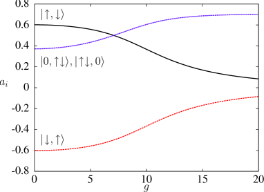
Figure 4: Coefficients $a_{i}$ (see Eq. (10)) for the ground state of the effective Hamiltonian $H_{\rm eff}$ in Eq. (5) (i.e. curve 1 in the right panel of Fig. 3) with $J=1$, $U=2$ and $\omega_{0}=50$. They cross very close to the crossing point of the eigenvalues in Fig. 3. The domination of the singlet states $|\!\uparrow,\downarrow\rangle$ at small couplings $g$ is changed by the domination of the dimer states for large values of $g$.

A nonzero tunneling lifts the degeneracies and leads to a unique ground state. The eigenvalues for nonzero tunneling and for $U=2$, $\omega_{0}=50$ are shown in Fig. 3. The two lowest excited states still cross at around $g\approx 7.1$, while the ground state is unique and thus the system does not exhibit the transition discussed in Sect. II. As a consequence of the polaron effect, the renormalized tunneling rates $\tau$, $K_{1}$, and $K_{2}$ vanish for large $g$. This implies for the eigenvalues the asymptotic behavior

$$\lambda_{1}\sim\lambda_{4}\sim-4g^{2}/\omega_{0},\ \ \ \lambda_{2}\sim\lambda_{3}\sim-2g^{2}/\omega_{0}\ .$$ (18)

This is also visible on the right panel of Fig. 3, while for the exact two sites problem with at most one phonon excitation (previous section), the eigenvalues do not merge for large coupling $g$ (cf. left panel of Fig. 3).

We plot the coefficients $a_{i}$ (see Eq. (10)) for the ground state of the effective Hamiltonian in Fig. 4. There is a crossover from the domination by the singlet states $|\!\uparrow,\downarrow\rangle$ (at small coupling $g$ when the effective interaction is repulsive, $\gamma>0$) to the domination of the doubly occupied states (at larger coupling $g$ when the effective interaction is attractive, $\gamma<0$).

To discuss the consequences of the crossing on observable dynamical quantities we study in the next section the dynamics of the quantum states and the spin imbalance of the LFA. This investigation includes the spectral density of the model.

V Dynamics in a double-well potential

The description of the dynamics of our quantum system is based on the knowledge of the energy levels, the initial quantum state and the overlap of the energy eigenstates with the initial quantum state. In other words, if the system with energy levels $E_{j}$ is prepared initially in state $|\Psi_{0}\rangle$, its quantum state $|\Psi_{t}\rangle$ evolves in time as

$$|\Psi_{t}\rangle=e^{-itH}|\Psi_{0}\rangle=\sum_{j}e^{-itE_{j}}|E_{j}\rangle\langle E_{j}|\Psi_{0}\rangle\ .$$ (19)

The energy levels $E_{j}$ and the overlap with the initial state $\langle E_{j}|\Psi_{0}\rangle$ can be described by spectral density. This will be discussed in the next section.

V.1 Spectral density

The return probability of the system to the initial state is calculated from the inverse Laplace transform of the projected resolvent of Eq. (4) as ziegler09

$$\langle\Psi_{0}|\Psi_{t}\rangle=\int_{\Gamma}e^{-izt}\langle\Psi_{0}|(z-H_{\rm{eff}}(z))^{-1}_{0}|\Psi_{0}\rangle\frac{dz}{2\pi i}\hskip 5.69046pt,$$ (20)

where the contour $\Gamma$ includes all the poles of the resolvent. The many-body spectral density is then given by

$$\rho_{\delta}(E)=-\frac{1}{\pi}{\rm Im}\langle\Psi_{0}|\bigl{(}z-H_{\rm{eff}}(z)\bigr{)}_{0}^{-1}|\Psi_{0}\rangle\hskip 5.69046pt,$$ (21)

where $z=E+i\delta$ and $\delta\ll 1$. For a finite dimensional Hilbert space it is a rational function with poles $z=E_{j}\,(j=0,1,2,...)$

$$\rho_{\delta}(E)=\delta\sum_{j}\frac{|\langle\Psi_{0}|E_{j}\rangle|^{2}}{(E-E_{j})^{2}+\delta^{2}}\hskip 5.69046pt.$$ (22)

This expression represents Lorentzian peaks at positions $E_{j}$ whose heights are $|\langle\Psi_{0}|E_{j}\rangle|^{2}/\delta$. Plotting $\rho_{\delta}(E)$ as a function of $E$, we can clearly identify the poles $E_{j}$ of the resolvent $G_{0}$ (see Eq. (4)) and the overlap between the energy state $|E_{j}\rangle$ and the initial state $|\Psi_{0}\rangle$. Here we calculate the spectral density for the initial state $|\Psi_{0}\rangle=|\!\uparrow,\downarrow\rangle$ for different coupling $g$. Then it should be noticed that the initial state is singly occupied and has no overlap with the doubly occupied eigenstate of Eq. (12). The results are shown in Fig. 5 for low energies. We observe three peaks, which correspond to the energies shown in Fig. 3. The central peak represents the dominant energy level for the dynamics. We notice the absence of one peak (corresponding to curve $3$ in Fig. 3), since the state $\bigl{(}|\!\uparrow\downarrow,0\rangle+|0,\uparrow\downarrow\rangle\bigl{)}/\sqrt{2}$ can not be reached from the initial state $\Psi_{0}=|\!\uparrow,\downarrow\rangle$. We also observe that before ($g=4$) and after ($g=10$) the crossing of the eigenvalues, there is one dominant central peak and two lower peaks. The characteristic frequencies of the dynamics are the differences of the energies of the central peak and the other ones. Close to the crossing point ($g=7.06$), the two other peaks are symmetric with respect to the central one. Consequently, only one frequency appears in the dynamics at the crossing point. This will also be seen in the spin imbalance of the next section. For big values of $g$ we observe two large peaks which are very close and a small peak far from the central peak. This implies a dominating small single frequency, as also found in the spin imbalance (cf. Fig. 8).

Figure 5: The spectral density in Eq. (22) for the initial state $|\Psi_{0}\rangle=|\!\uparrow,\downarrow\rangle$ and for $J=1$, $U=2$, $\omega_{0}=50$, $\delta=0.02$ and different values of the coupling $g$. We observe three peaks because the fourth eigenstate is orthogonal to the initial state. The central peak represents the dominant energy level and for big values of $g$ the contribution of one peak is very small. The frequencies of the spin imbalance are given by the difference between the dominant energy level and the other ones.

V.2 Spin imbalance

A recent experimental study of the dynamics of two spin-1/2 atoms with strong repulsion in a double well has revealed that, using two singly occupied wells as the initial state, the single occupation is static while the spin oscillates periodically between the two wells with two characteristic frequencies bloch07 ; bloch08 . This observation has been interpreted by an effective dynamics based on the Heisenberg model. The latter can be understood either within a strong-coupling approximation of the underlying Hubbard model bloch08 or within the recursive projection method for a general coupling ziegler09 . Experimentally this has been seen by measuring the spin imbalance between the two wells

$$N_{1,2}(t)~{}=~{}\frac{1}{2}\langle\Psi_{t}|n_{\uparrow 1}-n_{\downarrow 1}+n_{\downarrow 2}-n_{\uparrow 2}|\Psi_{t}\rangle\hskip 5.69046pt.$$ (23)

In our Holstein-Hubbard model we can vary the coupling $g$ between the LFA and the HA to realize an additional interaction. We have already seen in the spectral density that there is no overlap between the state of singly occupied wells and a state of a doubly occupied well. From this point of view we expect a similar behavior as found for the Hubbard model. However, there is the additional feature that we can tune continuously the local atom-atom coupling $\gamma$ from an attractive to a repulsive interaction. In this way we also reach a degeneracy point at which the effective interaction vanishes (i.e. $\gamma=0$). The existence of only three peaks in the spectral density of Fig. 5 explains the fact that the spin imbalance is characterized by only two frequencies, i.e., the difference between the dominant energy level and the other levels.

For $g=0$ we get the Fermi-Hubbard model without phonon excitations which corresponds with the above mentioned experiment. In this case, if the initial state is $|\uparrow,\downarrow\rangle$, the dynamics of spin imbalance is characterized by two frequencies, $U/2\left(\sqrt{(4J/U)^{2}+1}\pm 1\right)$ (see bloch08 ; ziegler09 ). The corresponding spin imbalance for $U=2$ is plotted in Fig. 6.

Figure 6: Spin imbalance $N_{1,2}(t)$ without inelastic scattering ($g=0$, left panel) and with strong inelastic scattering ($g=10$, right panel) for $J=1$, $U=2$ and $\omega_{0}=50$. There are two modes with frequencies $\omega_{1}\approx 3.24$ and $\omega_{2}\approx 1.24$ (left panel) and $\omega_{1}\approx 3.17$ and $\omega_{2}\approx 1.16$ (right panel) contribute to the dynamics.

Figure 7: Spin imbalance $N_{1,2}(t)$ at the level crossing $g=7.06541$ for $J=1$, $U=2$ and $\omega_{0}=50$. In this case only one mode with frequency $\omega_{1}\approx 1.96$ contributes to the dynamics.

For nonzero coupling $g$ the dynamics is affected by the presence of phonon excitations but it is still characterized by two frequencies, which are the differences between the second and the first and the second and the fourth curves in Fig. 3, respectively, i.e., $\omega_{1}=\lambda_{2}-\lambda_{3}$ and $\omega_{2}=\lambda_{2}-\lambda_{4}$. Consequently, at the crossing the dynamics of spin imbalance shows only one frequency since the differences between the curves in this case are equal, as depicted in Fig. 7. For larger couplings $g$ two frequencies component appear again as it is shown in the right panel of Fig. 6. Thus measuring the difference between the two frequencies, $\Delta=|\omega_{2}-\omega_{1}|$ provides a method to detect the crossing point experimentally: $\Delta$ vanishes at the crossing point as shown in Fig. 9 and the spin imbalance is characterized by only one frequency. Increasing the coupling $g$ further leaves a low frequency component with almost full amplitude and additional high-frequency modulation with small amplitude. This is depicted in Fig. 8. The low frequency component oscillates with the frequency $\omega_{2}\approx 4\tau^{2}/|\gamma|$, where $\tau$ is given in Eq. (6) and $\gamma=U-2g^{2}/\omega_{0}$. Thus $\omega_{2}\rightarrow 0$ as $g\rightarrow\infty$, which is a direct consequence of the polaron effect.

VI discussion and conclusion

At low energies, the restricted model with at most one phonon excitation per well has qualitatively the same behavior as the model with many phonon excitations, described by the effective Hamiltonian in Eq. (5). This is presented in Figs. 2 and 3, where the four lowest levels are plotted for both cases. The main difference, however, is that the Hilbert space of the model with many phonon excitations is much larger. Consequently, there are many excited states with energies higher than those shown in Figs. 2, 3. However, these states are not considered here because of their high energies. Due to the matrix elements $K_{1}$ and $K_{2}$ of the effective Hamiltonian in Eq. (11), these higher levels are closely related to harmonic oscillator levels with frequency $\omega_{0}$.

Without tunneling (i.e. $J=0$) there is a change of the ground state from single occupancy of the wells (weak coupling $g$) to double occupancy of one well (strong coupling $g$). This reflects the sign change of the effective coupling $\gamma=U-2g^{2}/\omega_{0}$. In the presence of tunneling (i.e. $J\neq 0$) the ground state, given by the coefficients of Eq. (15), changes smoothly upon a change of the coupling $g$. Its energy is the lowest solution of $\lambda_{3}(z)=z$, where $\lambda_{3}(z)$ is defined in Eq. (14). There is a transition due to the crossing of the first and second excited level though (cf. Fig. 3).

In conclusion, we have studied an atomic mixture of two heavy atoms and two light spin-1/2 fermionic atoms in a double-well potential, where the heavy atoms are subject to local harmonic oscillator potentials of the wells. This is modeled using the Holstein-Hubbard Hamiltonian, which is the simplest system that mimics the presence of phonons in a solid. We have applied the recursive projection method, which reduces the complexity of the full Hilbert space and leads to an effective fermionic Hamiltonian. We have found a transition for the the light fermions from singly occupied wells to doubly occupied wells as the coupling between heavy and light species is increased. This transition is manifested by the crossing of the second and third eigenvalue of the effective Hamiltonian. Moreover, the coupling between the light and the heavy atoms renormalizes the tunneling of light fermions between wells, which reflects the polaron effect. The dynamics is dominated by a spectral density with three peaks. This implies for the spin imbalance dynamics of the light atoms a periodic behavior with two characteristic frequencies. These frequencies coincide at the crossover of the two lowest excited states. Thus the oscillating behavior of the spin imbalance can be used to detect the crossing point experimentally.

Figure 8: Spin imbalance $N_{1,2}(t)$ for $g=20$, $J=1$, $U=2$ and $\omega_{0}=50$. Large coupling $g$ leaves a slow component with almost full amplitude and an additional high-frequency modulation with small amplitude. The slow component oscillates with the frequency $\omega_{2}\approx 4\tau^{2}/|\gamma|$. This is the direct consequence of the polaron effect, since it causes the single fermion tunneling decay exponentially, $\tau=Je^{-g^{2}/\omega_{0}^{2}}$.

Figure 9: Difference $\Delta=\bigl{|}\omega_{2}-\omega_{1}\bigr{|}$ between the frequencies of the modes contributing to the dynamics of spin imbalance. The difference disappears at the crossing point.

References

- (1) M. Lewenstein, A. Sanpera, V. Ahufinger, B. Damski, A. Sen, and U. Sen Adv. Phys., vol. 56, p. 243, 2007.
- (2) M. Greiner, O. Mandel, T. Esslinger, and I. B. T. Hänsch Nature, vol. 415, p. 39, 2002.
- (3) I. Bloch Nature Physics, vol. 1, p. 23, 2005.
- (4) S. Inouye, M. Andrews, J. Stenger, H.-J. Miesner, D. Stamper-Kurn, and W. Ketterle Nature, vol. 392, p. 151, 1998.
- (5) A. Görlitz, T. L. Gustavson, A. E. Leanhardt, R. Löw, A. P. Chikkatur, S. Gupta, S. Inouye, D. E. Pritchard, and W. Ketterle Phys. Rev. Lett., vol. 90, p. 090401, 2003.
- (6) O. Mandel, M. Greiner, A. Widera, T. Rom, T. W. Hänsch, and I. Bloch Phys. Rev. Lett., vol. 91, p. 010407, 2003.
- (7) H. Schmaljohann, M. Erhard, J. Kronjäger, M. Kottke, S. van Staa, L. Cacciapuoti, J. J. Arlt, K. Bongs, and K. Sengstock Phys. Rev. Lett., vol. 92, p. 040402, 2004.
- (8) M. Köhl, H. Moritz, T. Stöferle, K. Günter, and T. Esslinger Phys. Rev. Lett., vol. 94, p. 080403, 2005.
- (9) G. B. Partridge, W. Li, Y. A. Liao, and R. G. Hulet Phys. Rev. Lett., vol. 97, p. 190407, 2006.
- (10) M. Lewenstein, A. Sanpera, V. Ahufinger, B. Damski, A. Sen, and U. Sen Adv. Phys., vol. 56, p. 243, 2007.
- (11) K. E. Strecker, G. B. Partridge, and R. G. Hulet Phys. Rev. Lett., vol. 91, p. 080406, 2003.
- (12) H. Uys, T. Miyakawa, D. Meiser, and P. Meystre Phys. Rev. A, vol. 72, p. 053616, 2005.
- (13) C. A. Stan, M. W. Zwierlein, C. H. Schunck, S. M. F. Raupach, and W. Ketterle Phys. Rev. Lett., vol. 93, p. 143001, 2004.
- (14) K. Günter, T. Stöferle, H. Moritz, M. Köhl, and T. Esslinger Phys. Rev. Lett., vol. 96, p. 180402, 2006.
- (15) C. Ospelkaus, S. Ospelkaus, K. Bongs, and K. Sengstock Phys. Rev. Lett., vol. 96, p. 020401, 2006.
- (16) C. Maschler and H. Ritsch Phys. Rev. Lett., vol. 95, p. 260401, 2005.
- (17) J. Larson, B. Damski, G. Morigi, and M. Lewenstein Phys. Rev. Lett., vol. 100, p. 050401, 2008.
- (18) D.-W. Wang Phys. Rev. Lett., vol. 96, p. 140404, 2006.
- (19) I. Titvinidze, M. Snoek, and W. Hofstetter Phys. Rev. Lett., vol. 100, p. 100401, 2008.
- (20) D. Rokhsar and S. Kivelson Phys. Rev. Lett., vol. 61, p. 2376, 1988.
- (21) K. Ziegler Phys. Rev. A, vol. 77, p. 013623, 2008.
- (22) C. Xu and M. Fisher Phys. Rev. B, vol. 75, p. 104428, 2007.
- (23) M. Greiner, O. Mandel, T. Hänsch, and I. Bloch Nature, vol. 419, p. 51, 2002.
- (24) S. Fölling, S. Trotzky, P. Cheinet, M. Feld, R. Saers, A. Widera, T. Müller, and I. Bloch Nature, vol. 448, p. 1029, 2007.
- (25) S. Trotzky, P. Cheinet, S. Fölling, M. Feld, U. Schnorrberger, A. M. Rey, A. Polkovnikov, E. A. Demler, M. D. Lukin, and I. Bloch Science, vol. 319, p. 295, 2008.
- (26) J. Estève, C. Gross, A. Weller, S. Giovanazzi, and M. K. Oberthaler Nature, vol. 455, p. 1216, 2008.
- (27) K. Ziegler Phys. Rev. A, vol. 81, p. 034701, 2010.
- (28) A. Alexandrov and S. N. Mott, Polarons & Bipolarons. World Scientific, 1995.
- (29) J. Tempere, W. Casteels, M. Oberthaler, S. Knoop, E. Timmermans, and J. Devreese Phys. Rev. B, vol. 80, p. 184504, 2009.
- (30) E. Jaynes and F. Cummings Proc. IEEE, vol. 51, p. 89, 1963.
- (31) K. Ziegler Phys. Rev. A, vol. 68, p. 053602, 2003.
- (32) K. Ziegler Phys. Rev. B, vol. 74, p. 014301, 2006.