Smirnov’s fermionic observable away from criticality

Abstract

In a recent and celebrated article, Smirnov [Ann. of Math. (2) 172 (2010) 1435–1467] defines an observable for the self-dual random-cluster model with cluster weight $q=2$ on the square lattice $\mathbb{Z}^{2}$, and uses it to obtain conformal invariance in the scaling limit. We study this observable away from the self-dual point. From this, we obtain a new derivation of the fact that the self-dual and critical points coincide, which implies that the critical inverse temperature of the Ising model equals $\frac{1}{2}\log(1+\sqrt{2})$. Moreover, we relate the correlation length of the model to the large deviation behavior of a certain massive random walk (thus confirming an observation by Messikh [The surface tension near criticality of the 2d-Ising model (2006) Preprint]), which allows us to compute it explicitly.

T1Supported by the ANR Grant BLAN06-3-134462, the EU Marie-Curie RTN CODY, the ERC AG CONFRA, as well as by the Swiss FNS.

and

Introduction

The Ising model was introduced by Lenz Lenz as a model for ferromagnetism. His student, Ising, proved in his Ph.D. thesis Ising that the model does not exhibit any phase transition in one dimension. On the square lattice $\mathbb{L}=(\mathbb{Z}^{2},\mathbb{E})$, the Ising model is the first model where phase transition and non-mean-field behavior have been established (this was done by Peierls Peierls ).

An Ising configuration is a random assignment of spins $\{-1,1\}$ on $\mathbb{Z}^{2}$ such that the probability of a configuration $\sigma$ is proportional to $\exp[\beta\sum_{a\sim b}\sigma(a)\sigma(b)]$, where $\beta$ is the inverse temperature of the model and $a\sim b$ means that $(a,b)$ is an edge of the lattice, that is, $(a,b)\in\mathbb{E}$. Kramers and Wannier KramersWannier identified (without proof) the critical temperature where a phase transition occurs, separating an ordered from a disordered phase, using planar duality. In 1944, Kaufman and Onsager KaufmanOnsager computed the free energy of the model, paving the way to an analytic derivation of its critical temperature. In 1987, Aizenman, Barsky and Fernández AizenmanBarskyFernandez found a computation of the critical temperature based on differential inequalities. Both strategies are quite involved, and the first goal of this paper is to propose a new method, relying only on what we will call Smirnov’s observable:

Theorem 1

The critical inverse temperature of the Ising model on the square lattice $\mathbb{Z}^{2}$ is equal to

$$\beta_{c}=\tfrac{1}{2}\ln\bigl{(}1+\sqrt{2}\bigr{)}.$$

Beyond the determination of the critical inverse temperature, physicists and mathematicians were interested in estimates for the correlation between two spins, $\mathbb{E}_{\beta}[\sigma(a)\sigma(b)]$ (where $\mathbb{E}_{\beta}$ denotes the Ising measure). McCoy and Wu McCoyWu derived a closed formula for the two-point function, and an asymptotic analysis shows that it decays exponentially quickly when $\beta<\beta_{c}$. In addition to this, it was noticed by Messikh Messikh that the rate of decay is connected to large deviations estimates for the simple random walk. In this article, we present a direct derivation of this link, which provides a quick proof of the following theorem:

Theorem 2

Let $\beta<\beta_{c}$ and let $\mathbb{E}_{\beta}$ denote the (unique) infinite-volume Ising measure at inverse temperature $\beta$; fix $a=(a_{1},a_{2})\in\mathbb{L}$. Then

$$\lim_{n\rightarrow\infty}-\frac{1}{n}\ln(\mathbb{E}_{\beta}[\sigma(0)\sigma(na)])=a_{1}\mathop{\operatorname{arcsinh}}sa_{1}+a_{2}\mathop{\operatorname{arcsinh}}sa_{2},$$

where $s$ solves the equation

$$\sqrt{1+(sa_{1})^{2}}+\sqrt{1+(sa_{2})^{2}}=\sinh 2\beta+\sinh^{-1}2\beta.$$

Instead of working with the Ising model, we rather deal with its random-cluster representation (known as the random-cluster model with cluster weight $q=2$). It is well known FortuinKasteleyn that one can couple this model with the Ising model (see, e.g., Grimmett for a comprehensive study of random-cluster models) in such a way that the spin correlations of the Ising model get rephrased as cluster connectivity properties of their random-cluster representations, which allows for the use of geometric techniques. For instance, the determination of $\beta_{c}$ is equivalent to the determination of the critical point $p_{c}$ for the random-cluster model.

The understanding of the two-dimensional random-cluster model with $q=2$ has recently progressed greatly Smirnov , Duminil , thanks to the use of the so-called fermionic observable introduced by Smirnov Smirnov , which was instrumental in the proof of conformal invariance. This observable is defined on the edges of a finite domain with Dobrushin boundary conditions (mixed free and wired; see Section 1 for a formal definition), and it is discrete holomorphic at the self-dual point $p_{\mathrm{sd}}=\sqrt{2}/(1+\sqrt{2})$.

The idea of our argument is the following. Below the self-dual point, the observable can still be defined, but discrete holomorphicity fails, and the observable decays exponentially quickly in the distance to the wired boundary. Along the free boundary, the modulus of the observable can be written exactly as a connection probability, so in the $p<p_{\mathrm{sd}}$ regime the two-point function is exponentially small as well, and that implies that the system is then in the subcritical regime, thus providing the lower bound $p_{c}\geq p_{\mathrm{sd}}$ on the critical parameter. Theorem 1 then follows from duality.

In fact, the rate of exponential decay (and therefore Theorem 2) can be derived by comparing the observable to the Green function of a massive random walk (Proposition 15); the key ingredient is the observation that the observable is massive harmonic in the bulk for $p<p_{\mathrm{sd}}$. The correspondence between the two-point function of the Ising model and that of the massive random walk was previously noticed by Messikh Messikh .

In Section 1, we remind the reader of a few classic features of the random-cluster model. In Section 2, we define Smirnov’s observable away from criticality and gather some of its important properties—for instance, the fact that the observable on a graph is related to connection properties for sites on the boundary. In Section 3, we derive Theorem 1 by showing that the observable decays exponentially fast. Section 4 is devoted to a refinement of estimates on the observable, which leads to the proof of Theorem 2.

1 Basic features of the model

The Ising model on the square lattice admits a classical representation through the so-called random-cluster model with $q=2$. This model can be studied using geometric arguments which are classic in the theory of lattice models. We list here a few basic features of random-cluster models; a more exhaustive treatment (together with the proofs of all our statements) can be found in Grimmett’s monograph Grimmett . Readers familiar with the subject can skip directly to the next section.

Definition of the random-cluster model

The random-cluster measure can be defined on any graph. However, we will restrict ourselves to the square lattice, denoted by $\mathbb{L}=(\mathbb{Z}^{2},\mathbb{E})$ with $\mathbb{Z}^{2}$ denoting the set of sites and $\mathbb{E}$ the set of bonds. In this paper, $G$ will always denote a connected subgraph of $\mathbb{L}$, that is, a subset of vertices of $\mathbb{Z}^{2}$ together with all the bonds between them. We denote by $\partial G$ the (inner) boundary of $G$, that is, the set of sites of $G$ linked by a bond to a site of $\mathbb{Z}^{2}\setminus G$.

A configuration $\omega$ on $G$ is a random subgraph of $G$, having the same sites and a subset of its bonds. We will call the bonds belonging to $\omega$ open, the others closed. Two sites $a$ and $b$ are said to be connected (denoted by $a\leftrightarrow b$), if there is an open path—a path composed of open bonds only—connecting them. The (maximal) connected components will be called clusters. More generally, we extend this definition and notation to sets in a straightforward way.

A boundary condition $\xi$ is a partition of $\partial G$. We denote by $\omega\cup\xi$ the graph obtained from the configuration $\omega$ by identifying (or wiring) the vertices in $\xi$ that belong to the same class of $\xi$. A boundary condition encodes the way in which sites are connected outside of $G$. Alternatively, one can see it as a collection of abstract bonds connecting the vertices in each of the classes to each other. We still denote by $\omega\cup\xi$ the graph obtained by adding the new bonds in $\xi$ to the configuration $\omega$, since this will not lead to confusion. Let $o(\omega)$ [resp., $c(\omega)$] denote the number of open (resp., closed) bonds of $\omega$ and $k(\omega,\xi)$ the number of connected components of $\omega\cup\xi$. The probability measure $\phi^{\xi}_{p,q,G}$ of the random-cluster model on a finite subgraph $G$ with parameters $p\in[0,1]$ and $q\in(0,\infty)$ and boundary condition $\xi$ is defined by

$$\phi_{p,q,G}^{\xi}(\{\omega\}):=\frac{p^{o(\omega)}(1-p)^{c(\omega)}q^{k(\omega,\xi)}}{Z_{p,q,G}^{\xi}}$$ (1)

for any subgraph $\omega$ of $G$, where $Z_{p,q,G}^{\xi}$ is a normalizing constant known as the partition function. When there is no possible confusion, we will drop the reference to parameters in the notation.

The domain Markov property

One can encode, using an appropriate boundary condition $\xi$, the influence of the configuration outside a sub-graph on the measure within it. Consider a graph $G=(V,E)$ and a random-cluster measure $\phi^{\psi}_{p,q,G}$ on it. For $F\subset E$, consider $G^{\prime}$ with $F$ as the set of edges and the endpoints of it as the set of sites. Then, the restriction to $G^{\prime}$ of $\phi^{\psi}_{p,q,G}$ conditioned to match some configuration $\omega$ outside $G^{\prime}$ is exactly $\phi_{p,q,G^{\prime}}^{\xi}$, where $\xi$ describes the connections inherited from $\omega\cup\psi$ (two sites are wired if they are connected by a path in $\omega\cup\psi$ outside $G^{\prime}$; see (4.13) in Grimmett ). This property is the direct analog of the DLR conditions for spin systems.

Comparison of boundary conditions when $q\geq 1$

An event is called increasing if it is preserved by addition of open edges. When $q\geq 1$, the model is positively correlated (see (4.14) in Grimmett ), which has the following consequence: for any boundary conditions $\psi\leq\xi$ (meaning that $\psi$ is finer than $\xi$, or in other words, that there are fewer connections in $\psi$ than in $\xi$), we have

$$\phi^{\psi}_{p,q,G}(A)\leq\phi^{\xi}_{p,q,G}(A)$$ (2)

for any increasing event $A$. This last property, combined with the Domain Markov property, provides a powerful tool in order to study how events decorrelate.

Examples of boundary conditions: free, wired and Dobrushin

Two boundary conditions play a special role in the study of random-cluster models: the wired boundary condition, denoted by $\phi_{p,q,G}^{1}$, is specified by the fact that all the vertices on the boundary are pairwise connected; the free boundary condition, denoted by $\phi_{p,q,G}^{0}$, is specified by the absence of wirings between boundary sites. These boundary conditions are extremal for stochastic ordering, since any other boundary condition is smaller (resp., greater) than the wired (resp., free) boundary condition.

Another example of boundary condition will be very useful in this paper. The following definition is deliberately not as general as would be possible, in order to limit the introduction of notation. Let $G$ be a finite subgraph of $\mathbb{L}$; assume that its boundary is a self-avoiding polygon in $\mathbb{L}$, and let $a$ and $b$ be two sites of $\partial G$. The triple $(G,a,b)$ is called a Dobrushin domain. Orienting its boundary counterclockwise defines two oriented boundary arcs $ab$ and $ba$; the Dobrushin boundary condition is defined to be free on $ab$ (there are no wirings between boundary sites) and wired on $ba$ (all the boundary sites are pairwise connected). We will refer to those arcs as the free arc and the wired arc, respectively. The measure associated to this boundary condition will be denoted by $\phi_{p,q,G}^{a,b}$ or simply $\phi_{G}^{a,b}$.

Planar duality for Dobrushin domains

One can associate to any random-cluster measure with parameters $p$ and $q$ on a Dobrushin domain $(G,a,b)$ a dual measure. First, define the dual graph $G^{*}$ as follows: place a site in the center of every face of $G$ and every face of $\mathbb{L}$ adjacent to the free arc; see Figure 1. Bonds of the dual graph correspond to bonds of the primal graph and link nearest neighbors. Construct a bond

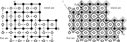
Figure 1: Left: a graph $G$ with its dual $G^{*}$. The black (resp., white) sites are the sites of $G$ (resp., $G^{*}$). The open bonds of $G$ (resp., $G^{*}$) are represented by solid (resp., dashed) black bonds. Right: construction of the medial lattice and the loop representation: the loops are interfaces between primal and dual clusters.

model on $G^{*}$ by declaring any bond of the dual graph to be open (resp., closed) if the corresponding bond of the primal lattice is closed (resp., open) for the initial random-cluster model. The new model on the dual graph is then a random-cluster measure with parameters $p^{*}=p^{*}(p,q)$ and $q^{*}=q$ satisfying

$$p^{*}(p,q):=\frac{(1-p)q}{(1-p)q+p}\quad\mbox{or equivalently}\quad\frac{p^{*}p}{(1-p^{*})(1-p)}=q$$

with wired boundary condition on the dual arc adjacent to $ab$, and free boundary condition on the dual arc adjacent to $ba$. In particular, it is again a random-cluster model with Dobrushin boundary condition. This relation is known as planar duality. It is then natural to define the self-dual point $p_{\mathrm{sd}}=p_{\mathrm{sd}}(q)$ by solving the equation $p^{*}(p_{\mathrm{sd}},q)=p_{\mathrm{sd}}$, which gives

$$p_{\mathrm{sd}}(q):=\frac{\sqrt{q}}{1+\sqrt{q}}.$$

This notion of duality has a natural counterpart, with the same formal definition, for free boundary conditions: the dual model is then a random-cluster model with parameters $p^{*}$ and $q$, with wired boundary condition.

Infinite-volume measures and the critical point

The domain Markov property and comparison between boundary conditions allow us to define infinite-volume measures. Indeed, one can consider a sequence of measures on boxes of increasing sizes with free boundary conditions. This sequence is increasing in the sense of stochastic domination, which implies that it converges weakly to a limiting measure, called the random-cluster measure on $\mathbb{L}$ with free boundary conditions (denoted by $\phi_{p,q}^{0}$). This classic construction can be performed with many other sequences of measures, defining a priori different infinite-volume measures on $\mathbb{L}$. For instance, one can define the random-cluster measure $\phi_{p,q}^{1}$ with wired boundary conditions, by considering the decreasing sequence of random-cluster measures on finite boxes with wired boundary condition.

For our purpose, the following example of infinite-volume measure will be important: we define a measure on the strip $\mathcal{S}_{\ell}=\mathbb{Z}\times[0,\ell]$. The sequence of measures $(\phi_{[-m,m]\times[0,{\ell}]}^{(m,0),(-m,0)})_{m\geq 0}$ is increasing, in the sense that for any cylindrical increasing event $A$ defined in the strip, the sequence $(\phi_{[-m,m]\times[0,{\ell}]}^{(m,0),(-m,0)}(A))$ is well defined for $m$ large enough and is nondecreasing. This implies that the sequence of measures converges weakly as $m$ goes to infinity. The limit is called the random-cluster measure on the infinite strip with free boundary conditions on the top and wired boundary condition on the bottom, and we will denote it by $\phi_{\mathcal{S}_{\ell}}^{\infty,-\infty}$.

When defining such measures in infinite volume by thermodynamical limits, it is natural to ask whether the limit depends on the choice of domains and boundary conditions used to build it; in the case of the random-cluster model, a more specific version of the question is whether taking free or wired boundary conditions affects the limit—these two being extremal, if the limits match, this implies uniqueness of the infinite-volume limit for all boundary conditions. It can be shown that for fixed $q\geq 1$, uniqueness can fail only on a countable set $\mathcal{D}_{q}$ of values of $p$; see Theorem (4.60) of Grimmett . From that (or rather from the weaker statement that the set of values of $p$ at which uniqueness holds is everywhere dense in $[0,1]$), and from the fact that measures for larger values of $p$ dominate those for smaller values, it is not difficult to show that there exists a critical point $p_{c}$ such that for any infinite-volume measure with $p<p_{c}$ (resp., $p>p_{c}$), there is almost surely no infinite component of connected sites (resp., at least one infinite component). Moreover, it is also known that the infinite-volume measure is unique when $p<p_{\mathrm{sd}}$.

Remark 1.1.

Physically, it is natural to conjecture that the critical point satisfies $p_{c}=p_{\mathrm{sd}}$. Indeed, if one assumes $p_{c}\neq p_{\mathrm{sd}}$, there should be a phase transition due to the change of behavior in the primal model at $p_{c}$ and a second (different) phase transition due to the change of behavior in the dual model at $p_{c}^{*}$. This is unlikely to happen—in fact, constructing a natural-looking model exhibiting two phase transitions is not so easy; but the equality of $p_{c}$ and $p_{\mathrm{sd}}$ is only known to hold in a few specific cases.

In the case of the random-cluster model on the square lattice, the authors proved recently BeffaraDuminil that indeed $p_{c}(q)=p_{\mathrm{sd}}(q)$ for all $q\geq 1$ (therefore determining the critical temperature for all $q$-state Potts models on $\mathbb{L}$). The argument does not use Smirnov’s observable, but it is quite a bit longer than the one we present here, is not as self-contained (mostly because it depends on recent sharp-threshold results by Graham and Grimmett GrahamGrimmett , GrahamGrimmett2 ) and it provides less information on the subcritical phase.

Coupling with the Ising model

The random-cluster model on $G$ with parameter $q=2$ is of particular interest since it can be coupled with the Ising model; consider a configuration $\omega$ sampled with probability $\phi_{p,2,G}^{0}$ and assign independently a spin $+1$ or $-1$ to every cluster with probability $1/2$. We are now facing a model of spins on sites of $G$. It can be proved that the law of the configuration corresponds to the Ising model at temperature $\beta=\beta(p)=-\frac{1}{2}\ln(1-p)$ with free boundary condition.

We are then equipped with a “dictionary” between the properties of the random-cluster model with $q=2$ and those of the Ising model. One instance of this relation is given by the useful identity

$$\mathbb{E}_{\beta(p),G}^{\mathrm{free}}[\sigma(0)\sigma(a)]=\phi_{p,2,G}^{0}(0\leftrightarrow a),$$ (3)

where the left-hand term denotes the correlation between sites $0$ and $a$ for the Ising model at inverse temperature $\beta$ on the graph $G$ with free boundary condition.

The critical inverse temperature $\beta_{c}$ of the Ising model is characterized by the fact that the two-point correlation undergoes a phase transition in its asymptotic behavior: below $\beta_{c}$, the correlation goes to 0 when $a$ goes to infinity, while above it, it stays bounded away from 0. The previous definition readily implies that $\beta_{c}=-\frac{1}{2}\log(1-p_{c}(2))$. In order to prove Theorem 1, it is thus sufficient to determine $p_{c}(2)$. Notice that the inverse temperature corresponding to the self-dual point is given by $\beta(p_{\mathrm{sd}})=\frac{1}{2}\ln(1+\sqrt{2})$ so that what needs to be proved can be written as $p_{c}(2)=p_{\mathrm{sd}}(2)$.

The same reasoning implies that we can compute correlation lengths for the random-cluster model in order to prove Theorem 2.

2 Definition of the observable

From now on, we consider only random-cluster models on the two-dimensional square lattice with parameter $q=2$ (we drop the dependency on $q$ in the notation).

The medial lattice and the loop representation

Let $(G,a,b)$ be a Dobrushin domain. In this paragraph, we aim for the construction of the loop representation of the random-cluster model, defined on the so-called medial graph. In order to do that, consider $G$ together with its dual $G^{*}$; declare black the sites of $G$ and white the sites of $G^{*}$. Replace every site with a colored diamond, as in Figure 1. The medial graph $G_{\diamond}=(V_{\diamond},E_{\diamond})$ is defined as follows (see Figure 1 again): $E_{\diamond}$ is the set of diamond sides which belong to both a black and a white diamond; $V_{\diamond}$ is the set of all the endpoints of the edges in $E_{\diamond}$. We obtain a subgraph of a rotated (and rescaled) version of the usual square lattice. We give $G_{\diamond}$ an additional structure as an oriented graph by orienting its edges clockwise around white faces.

The random-cluster measure with Dobrushin boundary condition has a rather convenient representation in this setting. Consider a configuration $\omega$: it defines clusters in $G$ and dual clusters in $G^{*}$. Through every vertex of the medial graph passes either an open bond of $G$ or a dual open bond of $G^{*}$. Hence, there is a unique way to draw Eulerian (i.e., using every edge of $E_{\diamond}$ exactly once) loops on the medial lattice such that the loops are the interfaces separating primal clusters from dual clusters. Namely, a loop arriving at a vertex of the medial lattice always makes a $\pm\pi/2$ turn so as not to cross the open or dual open bond through this vertex; see Figure 1 yet again.

Besides loops, the configuration will have a single curve joining the vertices adjacent to $a$ and $b$, which are the only vertices in $V_{\diamond}$ with three adjacent edges within the domain (the fourth edge emanating from $a$, resp., $b$, will be denoted by $e_{a}$, resp., $e_{b}$). This curve is called the exploration path; we will denote it by $\gamma$. It corresponds to the interface between the cluster connected to the wired arc and the dual cluster connected to the free arc.

This gives a bijection between random-cluster configurations on $G$ and Eulerian loop configurations on $G_{\diamond}$. The probability measure can be nicely rewritten (using Euler’s formula) in terms of the loop picture

$$\phi_{G}^{a,b}({\omega})=\frac{x(p)^{\#\ \mathrm{open}\ \mathrm{bonds}}\sqrt{2}{}^{\#\ \mathrm{loops}}}{\tilde{Z}(p,G)}\qquad\mbox{where }x(p):=\frac{p}{(1-p)\sqrt{2}},$$

and $\tilde{Z}(p,G)$ is a normalizing constant. Notice that $p=p_{\mathrm{sd}}$ if and only if $x(p)=1$. This bijection is called the loop representation of the random-cluster model. The orientation of the medial graph gives a natural orientation to the interfaces in the loop representation.

The edge observable for Dobrushin domains

Fix a Dobrushin domain $(G,a,b)$. Following Smirnov , we now define an observable $F$ on the edges of its medial graph, that is, a function $F\dvtx E_{\diamond}\to\mathbb{C}$. Roughly speaking, $F$ is a modification of the probability that the exploration path passes through an edge.

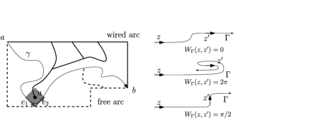
Figure 2: Left: a schematic picture of the exploration path and a boundary point $u$, together with two possible choices $e_{1}$ and $e_{2}$ for $e$. If $u$ is connected to the wired arc, the exploration path must go through $e$. Right: the winding of a curve. In the first example, the curve did one quarter-turn on the left and one quarter-turn on the right.

First, introduce the following definition: the winding $\mathrm{W}_{\Gamma}(z,z^{\prime})$ of a curve $\Gamma$ between two edges $z$ and $z^{\prime}$ of the medial graph is the total rotation (in radians and oriented counter-clockwise) that the curve makes from the mid-point of edge $z$ to that of edge $z^{\prime}$; see Figure 2. We define the observable $F$ for any edge $e\in E_{\diamond}$ as

$$F(e):=\phi_{G}^{a,b}\bigl{(}\mathrm{e}^{({\mathrm{i}}/{2})\mathrm{W}_{\gamma}(e,e_{b})}\mathbh{1}_{e\in\gamma}\bigr{)},$$ (4)

where $\gamma$ is the exploration path.

Remark 2.1.

In Smirnov , Smirnov extends the observable to vertices—as being the sum of $F$ on adjacent edges—in order to study the critical regime. Properly rescaled, this function converges to a holomorphic function, which is a key step toward the proof of conformal invariance; and indeed the exploration curve $\gamma$ converges to the trace of an SLE process as the mesh goes to $0$. Away from criticality, it is more convenient to work directly with the observable on edges.

The following three lemmas present the properties of the observable we will be using in the proofs of both theorems. They have direct counterparts in Smirnov’s article Smirnov (in particular, the idea of the proof of Lemma 2.2 can be found in the proof of Lemma 4.12 of Smirnov ), and as such they are not completely new. We still include their proofs here since our goal is to keep the present paper as self-contained as possible.

Lemma 2.2

Let $u\in G$ be a site on the free arc, and $e$ be a side of the black diamond associated to $u$ which borders a white diamond of the free arc; see Figure 2. Then

$$|F(e)|=\phi_{G}^{a,b}(u\leftrightarrow\mbox{wired arc}).$$ (5)

Let $u$ be a site of the free arc and recall that the exploration path is the interface between the open cluster connected to the wired arc and the dual open cluster connected to the free arc. Since $u$ belongs to the free arc, $u$ is connected to the wired arc if and only if $e$ is on the exploration path, so that

$$\phi_{G}^{a,b}(u\leftrightarrow\mbox{wired arc})=\phi_{G}^{a,b}(e\in\gamma).$$

The edge $e$ being on the boundary, the exploration path cannot wind around it, so that the winding (denoted $\mathrm{W}_{1}$) of the curve is deterministic (and easy to write in terms of that of the boundary itself). We deduce from this remark that

$$|F(e)| = \bigl{|}\phi_{G}^{a,b}\bigl{(}{\mathrm{e}}^{({\mathrm{i}}/{2})\mathrm{W}_{1}}\mathbh{1}_{e\in\gamma}\bigr{)}\bigr{|}=\bigl{|}{\mathrm{e}}^{({\mathrm{i}}/{2})\mathrm{W}_{1}}\phi_{G}^{a,b}(e\in\gamma)\bigr{|}$$

$$= \phi_{G}^{a,b}(e\in\gamma)=\phi_{G}^{a,b}(u\leftrightarrow\mbox{wired arc}).$$

For a random-cluster model, one can use the parameters $p$ or $x$ interchangeably. We introduce a third parameter which will be convenient: let $\alpha=\alpha(p)\in[0,2\pi)$ be given by the relation

$${\mathrm{e}}^{{\mathrm{i}}\alpha(p)}:=\frac{{\mathrm{e}}^{{\mathrm{i}}\pi/4}+x(p)}{{\mathrm{e}}^{{\mathrm{i}}\pi/4}x(p)+1}.$$ (6)

Observe that $\alpha(p)=0$ if and only if $p=p_{\mathrm{sd}}$ and $\alpha(p)>0$ for $p<p_{\mathrm{sd}}$. With this definition:

Lemma 2.3

Consider a vertex $v\in V_{\diamond}$ with four adjacent edges in $E_{\diamond}$. For every $p\in[0,1]$,

$$F(A)+F(C)={\mathrm{e}}^{{\mathrm{i}}\alpha(p)}[F(B)+F(D)],$$ (7)

where $A$ and $C$ (resp., $B$ and $D$) are the adjacent edges pointing toward (resp., away from) $v$, as depicted in Figure 3.

Let $v$ be a vertex of $V_{\diamond}$ with four adjacent edges, indexed as mention above. Edges $A$ and $C$ play symmetric roles, so that we can further require the indexation to be in clockwise order (see one such indexation in Figure 3). Recall that any vertex in $V_{\diamond}$ corresponds to a bond of the primal graph and a bond of the dual graph. We consider the involution $s$ on the space of configurations which switches the state (open or closed) of the bond of the primal lattice corresponding to $v$.

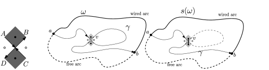
Figure 3: Left: indexation of the edges adjacent to $v$. Right: two associated configurations $\omega$ and $s(\omega)$. In this picture, $v$ corresponds to a vertical bond of the primal lattice.

Let $e$ be an edge of the medial graph and denote by $e_{\omega}:=\phi_{G}^{a,b}(\omega){\mathrm{e}}^{({\mathrm{i}}/{2})\mathrm{W}_{\gamma}(e,e_{b})}\times\mathbh{1}_{e\in\gamma}$ the contribution of $\omega$ to $F(e)$. Since $s$ is an involution, the following relation holds:

$$F(e):=\sum_{\omega}e_{\omega}=\frac{1}{2}\sum_{\omega}\bigl{[}e_{\omega}+e_{s(\omega)}\bigr{]}.$$

In order to prove (7), it suffices to prove the following for any configuration $\omega$:

$$A_{\omega}+A_{s(\omega)}+C_{\omega}+C_{s(\omega)}={\mathrm{e}}^{{\mathrm{i}}\alpha(p)}\bigl{(}B_{\omega}+B_{s(\omega)}+D_{\omega}+D_{s(\omega)}\bigr{)}.$$ (8)

When $\gamma(\omega)$ does not go through any of the edges adjacent to $v$, it is easy to see that neither does $\gamma(s(\omega))$. All the contributions then vanish and (8) trivially holds. Thus we can assume that $\gamma(\omega)$ passes through at least one edge adjacent to $v$. The interface follows the orientation of the medial graph, and thus can enter $v$ through either $A$ or $C$ and leave through $B$ or $D$. Without loss of generality we assume that it enters first through the edge $A$ and leaves last through the edge $D$; the other cases are treated similarly.

Two cases can occur: either the exploration curve, after arriving through $A$, leaves through $B$ and then returns a second time through $C$, leaving through $D$; or the exploration curve arrives through $A$ and leaves through $D$, with $B$ and $C$ belonging to a loop. Since the involution exchanges the two cases, we can assume that $\omega$ corresponds to the first case. Knowing the term $A_{\omega}$, it is possible to compute the contributions of $\omega$ and $s(\omega)$ to all of the edges adjacent to $v$. Indeed:

• The probability of $s(\omega)$ is equal to $x(p)\sqrt{2}$ times the probability of $\omega$ (due to the fact that there is one additional open edge and one additional loop).

• Windings of the curve can be expressed using the winding at $A$. For instance, the winding at $B$ in the configuration $\omega$ is equal to the winding at $A$ minus a $\pi/2$ turn.

The contributions are given as:

=315pt Configuration $\bolds{A}$ $\bolds{C}$ $\bolds{B}$ $\bolds{D}$ $\omega$ $A_{\omega}$ ${\mathrm{e}}^{{\mathrm{i}}\pi/2}A_{\omega}$ ${\mathrm{e}}^{-{\mathrm{i}}\pi/4}A_{\omega}$ ${\mathrm{e}}^{{\mathrm{i}}\pi/4}A_{\omega}$ $s(\omega)$ $x(p)\sqrt{2}A_{\omega}$ 0 0 ${\mathrm{e}}^{{\mathrm{i}}\pi/4}x(p)\sqrt{2}A_{\omega}$

Using the identity ${\mathrm{e}}^{{\mathrm{i}}\pi/4}+{\mathrm{e}}^{-{\mathrm{i}}\pi/4}=\sqrt{2}$, we deduce (8) by summing the contributions of all the edges around $v$.

The previous lemma provides us with one linear relation between values of $F$ for every vertex inside the domain. However, there are approximately twice as many edges than vertices in $G_{\diamond}$ so that these relations do not completely determine the value of $F$. The next lemma is therefore crucial since it decreases the number of possible values for $F$; roughly speaking, it states that the complex argument (modulo $\pi$) of $F(e)$ is determined by the orientation of the edge $e$.

Lemma 2.4

$F(e)$ belongs to $\mathbb{R}$ (resp., ${\mathrm{e}}^{-{\mathrm{i}}\pi/4}\mathbb{R}$, ${\mathrm{i}}\mathbb{R}$ or ${\mathrm{e}}^{{\mathrm{i}}\pi/4}\mathbb{R}$) on edges $e$ pointing in the same direction as the ending edge $e_{b}$ (resp., edges pointing in a direction which forms an angle $\pi/2$, $\pi$ and $3\pi/2$ with $e_{b}$).

The winding at an (oriented) edge can only take its value in the set $\mathrm{W}_{0}+2\pi\mathbb{Z}$ where $\mathrm{W}_{0}$ is the winding at $e$ of an arbitrary possible interface passing through $e$. Therefore, the winding weight involved in the definition of $F$ is always proportional to ${\mathrm{e}}^{{\mathrm{i}}\mathrm{W}_{0}/2}$ with a real-valued coefficient, and thus the complex argument of $F$ is equal to $\mathrm{W}_{0}/2$ or $\mathrm{W}_{0}/2+\pi$. Since $\mathrm{W}_{0}$ is exactly the angle between the direction of $e$ and that of $e_{b}$, we obtain the result.

The observable in strips

The definition of $F$ can be extended to the case of the strip. Indeed, the loop representation extends in this setting; the $\phi_{\mathcal{S}_{\ell}}^{\infty,-\infty}$-probability of having an infinite cluster is $0$: for fixed $\ell$, the model is essentially one dimensional, and it is a simple exercise to prove that it must be subcritical. Hence, there is a unique interface going from $+\infty$ to $-\infty$, which we call $\gamma$. We define

$$F(e):=\phi_{\mathcal{S}_{\ell}}^{\infty,-\infty}\bigl{[}{\mathrm{e}}^{({\mathrm{i}}/{2})\mathrm{W}_{\gamma}(e,-\infty)}\mathbh{1}_{e\in\gamma}\bigr{]},$$

where $\mathrm{W}_{\gamma}(e,-\infty)$ is the winding of the curve between $e$ and $-\infty$. This winding is well defined up to an additive constant, and we set it to be equal to $0$ for edges of the bottom side which point inside the domain. It is easy to see that $F$ is the limit of observables in finite boxes, so that the properties of fermionic observables in Dobrushin domains carry over to the infinite-volume case. In particular, the conclusions of the previous three lemmas apply to it as well.

3 Proof of Theorem 1

The proof consists of three steps:

• We first prove using Lemmas 2.3 and 2.4 that the observable decays exponentially fast when $p<p_{\mathrm{sd}}$ in a well chosen Dobrushin domain (namely a strip with free boundary condition on the top and wired boundary condition on the bottom). Lemma 2.2 then implies that the probability that a point on the top of the strip is connected to the bottom decays exponentially fast in the height of the strip.

• We derive exponential decay of the connectivity function for the infinite-volume measure with free boundary conditions from the first part.

• Finally, we show that exponential decay implies that the random-cluster model is subcritical when $p<p_{\mathrm{sd}}$, and that its dual is supercritical. This last step concludes the proof of Theorem 1 and is classical.

In the proof, points are identified with their complex coordinates.

Step 1: Exponential decay in the strip

Let $p<p_{\mathrm{sd}}$, and consider the random-cluster model on the strip $\mathcal{S}_{\ell}$ of height $\ell>0$ with wired boundary condition on the bottom and free boundary condition on the top. Define $e_{k}$ and $e_{k+1}$ to be the north-west-pointing sides of the diamonds associated to the points ${\mathrm{i}}k$ and ${\mathrm{i}}(k+1)$, respectively. Label some of the edges around these two diamonds as $x$, $x^{\prime}$, $x^{\prime\prime}$, $y$ and $y^{\prime}$ as shown in Figure 4.

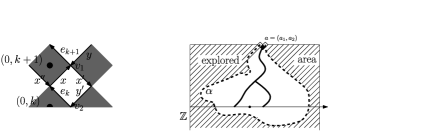
Figure 4: Left: the labeling of edges around $e_{k}$ used in Step 1. Right: a dual circuit surrounding an open path in the box $[-a_{2},a_{2}]^{2}$. Conditioning on to the most exterior such circuit gives no information on the state of the edges inside it.

Lemmas 2.3 and 2.4 have a very important consequence: around a vertex $v$, the value of the observable on one edge can be expressed in terms of its values on only two other edges. This can be done by seeing the relation given by Lemma 2.3 as a linear relation between four vectors in the plane $\mathbb{R}^{2}$, and applying an orthogonal projection to a line orthogonal to one of them (which can be chosen using Lemma 2.4). One then gets a linear relation between three real numbers, but using Lemma 2.4 “in reverse” shows that this is enough to determine any of the corresponding three (complex) values of the observable given the other two.

For instance, we can project (7) around $v_{1}$ orthogonally to $F(y)$, so that we obtain a relation between projections of $F(x)$, $F(x^{\prime})$ and $F(e_{k+1})$. Moreover, we know the complex argument (modulo $\pi$) of $F$ for each edge so that the relation between projections can be written as a relation between $F(x)$, $F(x^{\prime})$ and $F(e_{k+1})$ themselves. This leads to

$${\mathrm{e}}^{-{\mathrm{i}}\pi/4}F(x)=\cos(\pi/4-\alpha)F(e_{k+1})-\cos(\pi/4+\alpha){\mathrm{e}}^{-{\mathrm{i}}\pi/2}F(x^{\prime}).$$ (9)

Applying the same reasoning around $v_{2}$, we obtain

$${\mathrm{e}}^{-{\mathrm{i}}\pi/4}F(x)=\cos(\pi/4+\alpha)F(e_{k})-\cos(\pi/4-\alpha){\mathrm{e}}^{-{\mathrm{i}}\pi/2}F(x^{\prime\prime}).$$ (10)

The translation invariance of $\phi_{\mathcal{S}_{\ell}}^{\infty,-\infty}$ implies

$$F(x^{\prime})=F(x^{\prime\prime}).$$ (11)

Moreover, symmetry with respect to the imaginary axis implies that

$$F(x)={\mathrm{e}}^{{\mathrm{i}}\pi/4}\overline{F(x^{\prime})}={\mathrm{e}}^{-{\mathrm{i}}\pi/4}F(x^{\prime}).$$ (12)

Indeed, if, for a configuration $\omega$, $x$ belongs to $\gamma$, and the winding is equal to $W$, in the reflected configuration $\omega^{\prime}$, $x^{\prime}$ belongs to $\gamma(\omega^{\prime})$ and the winding is equal to $\pi/2-W$.

Plugging (11) and (12) into (9) and (10), we obtain

$$F(e_{k+1}) = {\mathrm{e}}^{-{\mathrm{i}}\pi/4}\frac{1+\cos(\pi/4+\alpha)}{\cos(\pi/4-\alpha)}F(x)$$

$$= \frac{[1+\cos(\pi/4+\alpha)]\cos(\pi/4+\alpha)}{[1+\cos(\pi/4-\alpha)]\cos(\pi/4-\alpha)}F(e_{k}).$$

Remember that $\alpha(p)>0$ since $p<p_{\mathrm{sd}}$, so that the multiplicative constant is less than 1. Using Lemma 2.2 and the previous equality inductively, we find that there exists $c_{1}=c_{1}(p)<1$ such that, for every $\ell>0$,

$$\phi_{\mathcal{S}_{\ell}}^{\infty,-\infty}[{\mathrm{i}}\ell\leftrightarrow\mathbb{Z}]=|F(e_{\ell})|=c_{1}^{\ell}|F(e_{1})|\leq c_{1}^{\ell},$$

where the last inequality is due to the fact that the observable has complex modulus less than $1$.

Step 2: Exponential decay for $\phi^{0}_{p}$ when $p<p_{\mathrm{sd}}$

Fix again $p<p_{\mathrm{sd}}$. Let $N\in\mathbb{N}$, and recall that $\phi^{0}_{p,N}:=\phi^{0}_{p,2,[-N,N]^{2}}$ converges to the infinite-volume measure with free boundary conditions $\phi^{0}_{p}$ when $N$ goes to infinity.

Consider a configuration in the box $[-N,N]^{2}$, and let $A_{\max}$ be the site of the cluster of the origin which maximizes the $\ell^{\infty}$-norm $\max\{|x_{1}|,|x_{2}|\}$ (it could be equal to $N$). If there is more than one such site, we consider the greatest one in lexicographical order. Assume that $A_{\max}$ equals $a=a_{1}+{\mathrm{i}}a_{2}$ with $a_{2}\geq|a_{1}|$ (the other cases can be treated the same way by symmetry, using the rotational invariance of the lattice).

By definition, if $A_{\max}$ equals $a$, $a$ is connected to $0$ in $[-a_{2},a_{2}]^{2}$. In addition to this, because of our choice of the free boundary condition, there exists a dual circuit starting from $a+\mathrm{i}/2$ in the dual of $[-a_{2},a_{2}]^{2}$ (which is the same as $\mathbb{L}^{*}\cap[-a_{2}-1/2,a_{2}+1/2]^{2}$) and surrounding both $a$ and $0$. Let $\Gamma$ be the outermost such dual circuit: we get

$$\phi_{p,N}^{0}(A_{\max}=a)=\sum_{\gamma}\phi_{p,N}^{0}(a\leftrightarrow 0|\Gamma=\gamma)\phi_{p,N}^{0}(\Gamma=\gamma),$$ (13)

where the sum is over contours $\gamma$ in the dual of $[-a_{2},a_{2}]^{2}$ that surround both $a$ and $0$.

The event $\{\Gamma=\gamma\}$ is measurable in terms of edges outside or on $\gamma$. In addition, conditioning on this event implies that the edges of $\gamma$ are dual-open. Therefore, from the domain Markov property, the conditional distribution of the configuration inside $\gamma$ is a random-cluster model with free boundary condition. Comparison between boundary conditions implies that the probability of $\{a\leftrightarrow 0\}$ conditionally on $\{\Gamma=\gamma\}$ is smaller than the probability of $\{a\leftrightarrow 0\}$ in the strip $\mathcal{S}_{a_{2}}$ with free boundary condition on the top and wired boundary condition on the bottom. Hence, for any such $\gamma$, we get

$$\phi_{p,N}^{0}(a\leftrightarrow 0|\Gamma=\gamma)\leq\phi_{\mathcal{S}_{a_{2}}}^{\infty,-\infty}(a\leftrightarrow 0)=\phi_{\mathcal{S}_{a_{2}}}^{\infty,-\infty}(a\leftrightarrow\mathbb{Z})\leq c_{1}^{a_{2}}=c_{1}^{|a|/2}$$

(observe that for the second measure, $\mathbb{Z}$ is wired, so that $\{a\leftrightarrow 0\}$ and $\{a\leftrightarrow\mathbb{Z}\}$ have the same probability). Plugging this into (13), we obtain

$$\phi_{p,N}^{0}(A_{\max}=a)\leq\sum_{\gamma}c_{1}^{|a|/2}\phi_{p,N}^{0}(\Gamma=\gamma)\leq c_{1}^{|a|/2}.$$

Fix $n\leq N$. Since $c_{1}<1$, we deduce from the previous inequality that there exist two constants $0<c_{2},C_{2}<\infty$ such that

$$\phi_{p,N}^{0}(0\leftrightarrow\mathbb{Z}^{2}\setminus[-n,n]^{2}) \leq \sum_{a\in[-N,N]^{2}\setminus[-n,n]^{2}}\phi_{p,N}^{0}(A_{\max}=a)$$

$$\leq \sum_{a\notin[-n,n]^{2}}c_{1}^{|a|/2}\leq C_{2}{\mathrm{e}}^{-c_{2}n}.$$

Since the estimate is uniform in $N$, we deduce that

$$\phi_{p}^{0}(0\leftrightarrow\mathbb{Z}^{2}\setminus[-n,n]^{2})\leq C_{2}{\mathrm{e}}^{-c_{2}n}.$$ (14)

Step 3: Exploiting exponential decay

The inequality $p_{c}\geq p_{\mathrm{sd}}$ follows from (14) since exponential decay prevents the existence of an infinite cluster for $\phi^{0}_{p}$ when $p<p_{\mathrm{sd}}$.

In order to prove that $p_{c}\leq p_{\mathrm{sd}}$, we use the following standard reasoning. Let $A_{n}$ be the event that the point $(n,0)$ is in an open circuit which surrounds the origin. Notice that this event is included in the event that the point $(n,0)$ is in a cluster of radius larger than $n$. For $p<p_{\mathrm{sd}}$, (14) implies that the probability of $A_{n}$ decays exponentially fast. The Borel–Cantelli lemma shows that there is almost surely only a finite number of values of $n$ such that $A_{n}$ occurs. In other words, there is only a finite number of open circuits surrounding the origin, which enforces the existence of an infinite dual cluster. It means that the dual model is supercritical whenever $p<p_{\mathrm{sd}}$. Equivalently, the primal model is supercritical whenever $p>p_{\mathrm{sd}}$, which implies $p_{c}\leq p_{\mathrm{sd}}$.

4 Proof of Theorem 2

In this section, we compute the correlation length in all directions. In Messikh , Messikh noticed that this correlation length was connected to large deviations for random walks and asked whether there exists a direct proof of the correspondence. Indeed, large deviations results are easy to obtain for random walks, so that one could deduce Theorem 2 easily. In the following, we exhibit what we believe to be the first direct proof of this result.

An equivalent way to deal with large deviations of the simple random walk is to study the massive Green function $G_{m}$, defined in the bulk as

$$G_{m}(x,y):=\mathbb{E}^{x}\biggl{[}\sum_{n\geq 0}m^{n}\mathbh 1_{X_{n}=y}\biggr{]},$$

where $\mathbb{E}^{x}$ is the law of a simple random walk starting at $x$.

The correlation length of the two-dimensional Ising model is the same as the correlation length for its random-cluster representation so that we will state the result in terms of the random-cluster. We use the parameters $p$ and $\alpha=\alpha(p)$ without revealing the connection with $\beta$ in the notation.

Proposition 4.1

For $p<p_{\mathrm{sd}}$ and any $a\in\mathbb{L}$,

$$-\lim_{n\rightarrow\infty}\frac{1}{n}\log\phi_{p}^{0}(0\leftrightarrow na)=-\lim_{n\rightarrow\infty}\frac{1}{n}\log G_{m}(0,na),$$ (15)

where $m=\cos[2\alpha(p)]$—the value of $\alpha(p)$ is given by (6).

In Messikh , the statement involves Laplace transforms, but we can translate it into the previous terms. Moreover, the mass is expressed in terms of $\beta$, but it is elementary to compute it in terms of $\alpha$. Theorem 2 follows from this proposition by first relating the two-point functions of the Ising and $q=2$ random-cluster models, as was mentioned earlier, and then deriving the asymptotics of the massive Green function explicitly—the details can be found, for instance, in the proof of Proposition 8 in Messikh .

Before delving into the actual proof, here is a short outline of the strategy we employ. We have already seen exponential decay in the strip, which was an essentially one-dimensional computation; we want to refine it into a two-dimensional version for correlations between two points $0$ and $a$ in the bulk, and once again we use the observable to estimate them. The basic step, namely obtaining local linear relations between the values of the observable, is the same, although it is complicated by the lack of translation invariance. The point is that the observable is massive harmonic when $p\neq p_{\mathrm{sd}}$ (see Lemma 4.2 below). Since $G_{m}(\cdot,\cdot)$ is massive harmonic in both variables away from the diagonal $x=y$, it is possible to compare both quantities.

The main problem is that we are interested in correlations in the bulk. The observable can be defined directly in the bulk (see below), but it provides only a lower bound on the correlations. In order to obtain an upper bound, we have to introduce an “artificial” domain [that will be $T(a)$ below], which needs two features: the observable in it can be well estimated, and at the same time correlations inside it have comparable probabilities to correlations in the bulk. For the second one, it is equivalent to impose that the Wulff shape centered at $0$, and having $a$ on its boundary is contained in the domain in the neighborhood of $a$; from convexity, it is then natural to construct $T(a)$ as the whole plane minus two wedges, one with vertex at $0$ and the other with vertex at $a$.

The proof is rather technical since we need to deal with the behavior of the observable on the boundary of the domains. This was also an issue in Smirnov’s proof. At criticality, the difficulty was overcome by working with the discrete primitive $H$ of $F^{2}$. Unfortunately, there is no nice equivalent of $H$ to work with away from criticality. The solution is to use a representation of $F$ in terms of a massive random walk. This representation extends to the boundary and allows to control the behavior of $F$ everywhere. Proof of Theorem 2 Let $p<p_{\mathrm{sd}}$. Without loss of generality, we can consider $a=(a_{1},a_{2})\in\mathbb{L}$ satisfying $a_{2}\geq a_{1}\geq 0$. In the proof, we identify a site $u$ of $\mathbb{L}$ with the unique side $e_{u}$ of the associated black diamond which points north-west. In other words $F(u)$ and $\{u\in\gamma\}$ should be understood as $F(e_{u})$ and $\{e_{u}\in\gamma\}$—notice that this differs from the notation used in Smirnov .

The lower bound. Consider the observable $F$ in the bulk defined as follows: for every edge $e$ not equal to $e_{0}$,

$$F(e):=\phi_{p}^{0}\bigl{(}{\mathrm{e}}^{({\mathrm{i}}/{2})\mathrm{W}_{\gamma}(e,e_{0})}\mathbh{1}_{e\in\gamma}\bigr{)},$$ (16)

where $\gamma$ is the unique loop passing through $e_{0}$. Note that this definition is justified by the fact that $p$ is subcritical, and that it immediately implies that

$$\phi_{p}^{0}(0\leftrightarrow a)\geq|F(a)|.$$ (17)

We mention that $F$ is not well defined at $e_{0}$. Indeed, $e_{0}$ can be thought of as the start of the loop $\gamma$ or its end. In other words, $F$ is multi-valued at $e_{0}$, with value 1 or $-$1.

Lemma 2.3 can be extended to this context following a very similar proof, but taking into account that $F$ is multi-valued at $e_{0}$. More precisely, let $e_{0}=xy$. Around any vertex $v\notin\{x,y\}$ the relation in Lemma 2.3 still holds; besides,

$$\cases{F(\mathit{SE})+1={\mathrm{e}}^{{\mathrm{i}}\alpha(p)}[F(\mathit{SW})+F(\mathit{NE})],&\quad if $v=y$,\vspace*{2pt}\cr F(\mathit{SW})+F(\mathit{NE})={\mathrm{e}}^{{\mathrm{i}}\alpha(p)}[-1+F(\mathit{SE})],&\quad if $v=x$,}$$

where the $\mathit{NE}$ (resp., $\mathit{SE}$, $\mathit{SW}$) is the edge at $v$ pointing to the north-east (resp., south-east, south-west). In other words, the statement of Lemma 2.3 still formally holds if we choose the convention that $F(e_{0})=1$ when considering the relation around $x$, and $F(e_{0})=-1$ when considering the relation around $y$.

One can see that Lemma 2.4 is still valid. In fact, the two lemmas imply that $F$ is massive harmonic:

Lemma 4.2

Let $p<p_{\mathrm{sd}}$ and consider the observable $F$ in the bulk. For any site $X$ not equal to 0, we have

$$\Delta_{\alpha}F(X):=\frac{\cos 2\alpha}{4}[F(W)+F(S)+F(E)+F(N)]-F(X)=0,$$

where $W$, $S$, $E$ and $N$ are the four neighbors of $X$.

Consider a site $X$ inside the domain and recall that we identify $X$ with the corresponding edge of the medial lattice pointing north-west. Index the edges around $X$ in the same way as in case 1 of Figure 5. By considering the six equations

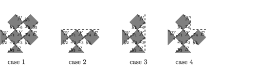
Figure 5: Indexation of the edges around vertices in the different cases.

corresponding to vertices that end one of the edges $x_{1},\ldots,x_{6}$ (being careful to identify the edges $A$, $B$, $C$ and $D$ correctly for each of the vertices), we obtain the following linear system:

$$\cases{F(X)+F(y_{1})={\mathrm{e}}^{{\mathrm{i}}\alpha}[F(x_{1})+F(x_{6})],\vspace*{1pt}\cr F(y_{2})+F(x_{1})={\mathrm{e}}^{{\mathrm{i}}\alpha}[F(x_{2})+F(W)],\vspace*{1pt}\cr F(S)+F(x_{2})={\mathrm{e}}^{{\mathrm{i}}\alpha}[F(y_{3})+F(x_{3})],\vspace*{1pt}\cr F(x_{3})+F(x_{4})={\mathrm{e}}^{{\mathrm{i}}\alpha}[F(y_{4})+F(X)],\vspace*{1pt}\cr F(E)+F(x_{5})={\mathrm{e}}^{{\mathrm{i}}\alpha}[F(x_{4})+F(y_{5})],\vspace*{1pt}\cr F(x_{6})+F(y_{6})={\mathrm{e}}^{{\mathrm{i}}\alpha}[F(x_{5})+F(N)].}$$

Recall that by definition, $F(X)$ is real. For an edge $e$, denote by $f(e)$ the projection of $F(e)$ on the line directed by its argument ($\mathbb{R}$, ${\mathrm{e}}^{{\mathrm{i}}\pi/4}\mathbb{R}$, $i\mathbb{R}$ and ${\mathrm{e}}^{-{\mathrm{i}}\pi/4}\mathbb{R}$). By projecting orthogonally to the $F(y_{i})$, $i=1,\ldots,6$, the system becomes

$$\cases{f(X)=\cos(\pi/4+\alpha)f(x_{1})+\cos(\pi/4-\alpha)f(x_{6}),&(1)\vspace*{1pt}\cr f(x_{1})=\cos(\pi/4+\alpha)f(x_{2})+\cos(\pi/4-\alpha)f(W),&(2)\vspace*{1pt}\cr f(x_{3})=\cos(\pi/4-\alpha)f(S)+-\cos(\pi/4+\alpha)f(x_{2}),&(3)\vspace*{1pt}\cr f(X)=\cos(\pi/4+\alpha)f(x_{3})+\cos(\pi/4-\alpha)f(x_{4}),&(4)\vspace*{1pt}\cr f(x_{4})=\cos(\pi/4+\alpha)f(E)+\cos(\pi/4-\alpha)f(x_{5}),&(5)\vspace*{1pt}\cr f(x_{6})=-\cos(\pi/4-\alpha)f(x_{5})+\cos(\pi/4+\alpha)f(N).&(6)}$$

By adding $(2)$ to $(3)$, $(5)$ to $(6)$ and $(1)$ to $(4)$, we find

$$\cases{f(x_{3})+f(x_{1})=\cos(\pi/4-\alpha)[f(W)+f(S)],&(7)\vspace*{1pt}\cr f(x_{6})+f(x_{4})=\cos(\pi/4+\alpha)[f(E)+f(N)],&(8)\vspace*{1pt}\cr 2f(X)=\cos(\pi/4+\alpha)[f(x_{3})+f(x_{1})]+\cos(\pi/4-\alpha)[f(x_{6})+f(x_{4})].&(9)}$$

Plugging $(7)$ and $(8)$ into $(9)$, we obtain

$$2f(X)=\cos(\pi/4+\alpha)\cos(\pi/4-\alpha)[f(W)+f(S)+f(E)+f(N)].$$

The edges $X,\ldots,N$ are pointing in the same direction so the previous equality becomes an equality with $F$ in place of $f$ (use Lemma 2.4). A simple trigonometric identity then leads to the claim.

Define the Markov process with generator $\Delta_{\alpha}$, which one can see either as a branching process or as the random walk of a massive particle. We choose the latter interpretation and write this process $(X_{n},m_{n})$ where $X_{n}$ is a random walk with jump probabilities defined in terms of $\Delta_{\alpha}$—the proportionality between jump probabilities is the same as the proportionality between coefficients—and $m_{n}$ is the mass associated to this random walk. The law of the random walk starting at $x$ is denoted $\mathbb{P}^{x}$. Note that the mass of the walk decays by a factor $\cos 2\alpha$ at each step.

Denote by $\tau$ the hitting time of $0$. The last lemma translates into the following formula for any $a$ and any $t$:

$$F(a)=\mathbb{E}^{a}[F(X_{t\wedge\tau})m_{t\wedge\tau}].$$ (18)

The sequence $(F(X_{t})m_{t})_{t\leq\tau}$ is obviously uniformly integrable, so that (18) can be improved to

$$F(a)=\mathbb{E}^{a}[F(X_{\tau})m_{\tau}].$$ (19)

Equations (17), (19) together with Lemma 4.3 below give

$$\phi_{p}^{0}(0\leftrightarrow a)\geq\frac{c}{|a|}G_{\cos 2\alpha}(0,a),$$

which implies the lower bound.

Lemma 4.3

There exists $c>0$ such that, for every $a$ in the upper-right quadrant,

$$|\mathbb{E}^{a}[F(X_{\tau})m_{\tau}]|\geq\frac{c}{|a|}G_{\cos 2\alpha}(0,a).$$

Recall that $F(X_{\tau})$ is equal to 1 or $-1$ depending on the last step the walk takes before reaching 0. Let us rewrite $\mathbb{E}^{a}[F(X_{\tau})m_{\tau}]$ as

$$\mathbb{E}^{a}\bigl{[}m^{\tau}1_{\{X_{\tau-1}=W\ \mathrm{or}\ S\}}\bigr{]}-\mathbb{E}^{a}\bigl{[}m^{\tau}1_{\{X_{\tau-1}=N\ \mathrm{or}\ E\}}\bigr{]}.$$

Now, let $\Delta_{\alpha}$ be the line $y=-x$, and let $T$ be the time of the last visit of $\Delta_{\alpha}$ by the walk before time $\tau$ (set $T=\infty$ if it does not exist). On the event that $X_{\tau-1}=W$ or $S$, this time is finite, and reflecting the part of the path between $T$ and $\tau$ across $\Delta_{\alpha}$ produces a path from $a$ to $0$ with $X_{\tau-1}=E$ or $N$. This transformation is one-to-one, so summing over all paths, we obtain

$$\mathbb{E}^{a}\bigl{[}m^{\tau}1_{\{X_{\tau-1}=W\ \mathrm{or}\ S\}}\bigr{]}-\mathbb{E}^{a}\bigl{[}m^{\tau}1_{\{X_{\tau-1}=N\ \mathrm{or}\ E\}}\bigr{]}$$

$$\qquad=-\mathbb{E}^{a}\bigl{[}m^{\tau}1_{\{X_{\tau-1}=N\ \mathrm{or}\ E\}}1_{\{T=\infty\}}\bigr{]},$$

which in turn is equal to $-\mathbb{E}^{a}[m^{\tau}1_{\{T=\infty\}}]$. General arguments of large deviation theory imply that $\mathbb{E}^{a}[m^{\tau}1_{\{T=\infty\}}]\geq\frac{c}{|a|}G_{\cos 2\alpha}(0,a)$ for some universal constant $c$.

The upper bound. Assume that $0$ is connected to $a$ in the bulk. We first show how to reduce the problem to estimations of correlations for points on the boundary of a domain.

For every $u=u_{1}+{\mathrm{i}}u_{2}$ and $v=v_{1}+{\mathrm{i}}v_{2}$ two sites of $\mathbb{L}$, write $u\prec v$ if $u_{1}<v_{1}$ and $u_{2}<v_{2}$. This relation is a partial ordering of $\mathbb{L}$. We consider the following sets:

$$\mathbb{L}^{+}(u)=\{x\in\mathbb{L}\dvtx u\prec x\}\quad\mbox{and}\quad\mathbb{L}^{-}=\{x\in\mathbb{L}\dvtx x\prec 0\}$$

and

$$T(u)=\mathbb{L}\setminus\bigl{(}\mathbb{L}^{+}(u)\cup\mathbb{L}^{-}\bigr{)}.$$

In the following, $L^{+}(u)$ and $L^{-}$ will denote the interior boundaries of $T(u)$ near $\mathbb{L}^{+}(u)$ and $\mathbb{L}^{-}$, respectively; see Figure 6. The measure with wired boundary conditions on $\mathbb{L}^{-}$ and free boundary conditions on $\mathbb{L}^{+}(u)$ is denoted $\phi_{T(u)}$.

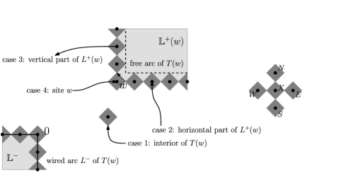
Figure 6: The set $T(w)$. The different cases listed in the definition of the Laplacian are pictured.

Assume that $a$ is connected to 0 in the bulk. By conditioning on $w$ which maximizes the partial $\succ$-ordering in the cluster of $0$ (it is the same reasoning as in Section 3), we obtain the following:

$$\phi_{p}^{0}(a\leftrightarrow 0)\leq\sum_{w\succ a}\phi_{T(w)}(w\leftrightarrow\mathbb{L}^{-})\leq C_{3}|a|\max_{w\succ a,|w|\leq c_{3}|a|}\phi_{T(w)}(w\leftrightarrow\mathbb{L}^{-})$$ (20)

for $c_{3},C_{3}$ large enough. The existence of $c_{3}$ is given by the fact that the two-point function decays exponentially fast: a priori estimates on the correlation length show that the maximum above cannot be reached at any $w$ which is much further away from the origin than $a$, and even that the sum of the corresponding probabilities is actually of a smaller order than the remaining terms. Summarizing, it is sufficient to estimate the probability of the right-hand side of (20).

Observe that $w$ is on the free arc of $T(w)$, so that, harnessing Lemma 2.2, we find

$$\phi_{T(w)}(w\leftrightarrow L^{-})=|F(w)|,$$ (21)

where $F$ is the observable in the Dobrushin domain $T(w)$ (the winding is fixed in such a way that it equals 0 at $e_{w}$). Now, similarly to Lemma 4.2, $F$ satisfies local relations in the domain $T(w)$:

Lemma 4.4

The observable $F$ satisfies $\Delta_{\alpha}F=0$ for every site not on the wired arc, where the massive Laplacian $\Delta_{\alpha}$ on $T(w)$ is defined by the following relations: for all $g\dvtx T(w)\mapsto\mathbb{R}$, $(g+\Delta_{\alpha}g)(X)$ is equal to

$$\frac{\cos 2\alpha}{4}[g(W)+g(S)+g(E)+g(N)]$$

inside the domain;

$$\frac{\cos 2\alpha}{2(1+\cos(\pi/4-\alpha))}[g(W)+g(S)]+\frac{\cos(\pi/4+\alpha)}{1+\cos(\pi/4-\alpha)}g(E)$$

on the horizontal part of $L^{+}(w)$;

$$\frac{\cos 2\alpha}{2(1+\cos(\pi/4-\alpha))}[g(W)+g(S)]+\frac{\cos(\pi/4+\alpha)}{1+\cos(\pi/4-\alpha)}g(N)$$

on the vertical part of $L^{+}(w)$;

$$\frac{\cos 2\alpha}{4}[g(W)+g(S)]+\frac{\cos(\pi/4-\alpha)}{2}[g(E)+g(N)]\qquad\mbox{at }w$$

with $N$, $E$, $S$ and $W$ being the four neighbors of $X$.

When the site is inside the domain, the proof is the same as in Lemma 4.2. For boundary sites, a similar computation can be done. For instance, consider case 2 in Figure 5. Equations (3) and (7) in the proof of Lemma 4.2 are preserved. Furthermore, Lemma 2.2 implies that

$$f(X)=f(x_{1})=\phi_{T(w)}(X\leftrightarrow L^{-})$$

and similarly $f(x_{4})=f(E)$ (where $f$ is still as defined in the proof of Lemma 4.2). Plugging all these equations together, we obtain the second equality. The other cases are handled similarly.

Now, we aim to use a representation with massive random walks similar to the proof of the lower bound. One technical point is the fact that the mass at $w$ is larger than 1. This could a priori prevent $(F(X_{t})m_{t})_{t}$ from being uniformly integrable. Therefore, we need to deal with the behavior at $w$ separately. Denote by $\tau_{1}$ the hitting time (for $t>0$) of $w$, and by $\tau$ the hitting time of $L^{-}$. Since the masses are smaller than 1, except at $w$, $(F(X_{t})m_{t})_{t\leq\tau\wedge\tau_{1}}$ is uniformly integrable and we can apply the stopping theorem to obtain

$$F(w)=\mathbb{E}^{w}[F(X_{\tau\wedge\tau_{1}})m_{\tau\wedge\tau_{1}}]=\mathbb{E}^{w}[F(X_{\tau_{1}})m_{\tau_{1}}\mathbh{1}_{\tau_{1}<\tau}]+\mathbb{E}^{w}[F(X_{\tau})m_{\tau}\mathbh{1}_{\tau<\tau_{1}}].$$

Since $X_{\tau_{1}}=w$, the previous formula can be rewritten as

$$F(w)=\frac{\mathbb{E}^{w}[F(X_{\tau})m_{\tau}\mathbh{1}_{\tau<\tau_{1}}]}{1-\mathbb{E}^{w}(m_{\tau_{1}}\mathbh{1}_{\tau_{1}<\tau})}.$$ (22)

When $w$ goes to infinity in a prescribed direction, $[1-\mathbb{E}^{w}(m_{\tau_{1}}\mathbh{1}_{\tau_{1}<\tau})]$ converges to the analytic function $h\dvtx[0,1]\rightarrow\mathbb{R},p\mapsto 1-\mathbb{E}^{w}(m_{\tau_{1}})$ (since the function is translation-invariant). The function $h$ is not equal to 0 when $p=0$, implying that it is equal to 0 for a discrete set $\mathcal{P}$ of points. In particular, for $p\notin\mathcal{P}$, the first term in the right-hand side stays bounded when $w$ goes to infinity. Denoted by $C_{4}=C_{4}(p)$ such a bound. Recalling that $|F|\leq 1$ and that the mass is smaller than 1 except at $w$, (22) becomes

$$|F(w)| \leq C_{4}|\mathbb{E}^{w}[F(X_{\tau})m_{\tau}\mathbh{1}_{\tau<\tau_{1}}]|\leq\mathbb{E}^{w}[m_{\tau}\mathbh{1}_{\tau<\tau_{1}}]$$

$$\leq C_{4}\sum_{w\prec x}\mathbb{E}^{x}\bigl{[}(\cos 2\alpha)^{\tau}\mathbh{1}_{\tau<\tau_{1}}1_{\{(X_{t})\ \mathrm{avoids}\ L^{+}(w)\}}\bigr{]}$$

$$\leq C_{4}\sum_{w\prec x}G_{\cos 2\alpha}(0,x),$$

where the last inequality is due to the fact that we release the condition on avoiding $L^{+}(w)$.

Finally, it only remains to bound the right-hand side. From (4), we deduce

$$|F(w)|\leq C_{5}|w|G_{\cos 2\alpha}(0,w),$$ (25)

where the existence of $C_{5}$ is due to the exponential decay of $G_{\cos 2\alpha}(\cdot,\cdot)$ and the fact that $G_{\cos 2\alpha}(0,x)\leq G_{\cos 2\alpha}(0,w)$ whenever $w\prec x$. We deduce from (20), (21) and (25) that

$$\qquad\phi_{p}(0\leftrightarrow a)\leq C_{3}C_{5}|a|^{2}\max_{w\succ a,|w|_{\infty}\leq c_{5}|a|_{\infty}}G_{m}(0,w)\leq C_{6}|a|^{2}G_{m}(0,a).$$ (26)

Taking the logarithm, we obtain the claim for all $p<p_{\mathrm{sd}}$ not in the discrete set $\mathcal{P}$. The result follows for every $p$ using the fact that the correlation length is increasing in $p$.

References

- (1) {barticle}[mr] \bauthor\bsnmAizenman, \bfnmM.\binitsM., \bauthor\bsnmBarsky, \bfnmD. J.\binitsD. J. and \bauthor\bsnmFernández, \bfnmR.\binitsR. (\byear1987). \btitleThe phase transition in a general class of Ising-type models is sharp. \bjournalJ. Stat. Phys. \bvolume47 \bpages343–374. \biddoi=10.1007/BF01007515, issn=0022-4715, mr=0894398 \bptokimsref \endbibitem
- (2) {barticle}[auto:STB—2012/02/03—11:55:16] \bauthor\bsnmBeffara, \bfnmV.\binitsV. and \bauthor\bsnmDuminil-Copin, \bfnmH.\binitsH. (\byear2012). \btitleThe self-dual point of the two-dimensional random-cluster model is critical for . \bjournalProbab. Theory Related Fields \bvolume153 \bpages511–542. \bidmr=2948685 \bptokimsref \endbibitem
- (3) {barticle}[auto:STB—2012/02/03—11:55:16] \bauthor\bsnmDuminil-Copin, \bfnmH.\binitsH., \bauthor\bsnmHongler, \bfnmC.\binitsC. and \bauthor\bsnmNolin, \bfnmP.\binitsP. (\byear2012). \btitleConnection probabilities and RSW-type bounds for the two-dimensional FK Ising model. \bjournalComm. Pure Appl. Math. \bvolume64 \bpages1165–1198. \bidmr=2839298 \bptokimsref \endbibitem
- (4) {barticle}[mr] \bauthor\bsnmFortuin, \bfnmC. M.\binitsC. M. and \bauthor\bsnmKasteleyn, \bfnmP. W.\binitsP. W. (\byear1972). \btitleOn the random-cluster model. I. Introduction and relation to other models. \bjournalPhysica \bvolume57 \bpages536–564. \bidmr=0359655 \bptokimsref \endbibitem
- (5) {barticle}[mr] \bauthor\bsnmGraham, \bfnmB. T.\binitsB. T. and \bauthor\bsnmGrimmett, \bfnmG. R.\binitsG. R. (\byear2006). \btitleInfluence and sharp-threshold theorems for monotonic measures. \bjournalAnn. Probab. \bvolume34 \bpages1726–1745. \biddoi=10.1214/009117906000000278, issn=0091-1798, mr=2271479 \bptokimsref \endbibitem
- (6) {barticle}[auto:STB—2012/02/03—11:55:16] \bauthor\bsnmGraham, \bfnmB. T.\binitsB. T. and \bauthor\bsnmGrimmett, \bfnmG. R.\binitsG. R. (\byear2011). \btitleSharp thresholds for the random-cluster and Ising models. \bjournalAnn. Appl. Probab. \bvolume21 \bpages240–265. \bidmr=2759201 \bptokimsref \endbibitem
- (7) {bbook}[mr] \bauthor\bsnmGrimmett, \bfnmGeoffrey\binitsG. (\byear2006). \btitleThe Random-Cluster Model. \bseriesGrundlehren der Mathematischen Wissenschaften [Fundamental Principles of Mathematical Sciences] \bvolume333. \bpublisherSpringer, \baddressBerlin. \biddoi=10.1007/978-3-540-32891-9, mr=2243761 \bptokimsref \endbibitem
- (8) {barticle}[auto:STB—2012/02/03—11:55:16] \bauthor\bsnmIsing, \bfnmE.\binitsE. (\byear1925). \btitleBeitrag zur theorie des ferromagnetismus. \bjournalZ. Phys. \bvolume31 \bpages253–258. \bptokimsref \endbibitem
- (9) {bmisc}[auto:STB—2012/02/03—11:55:16] \bauthor\bsnmKaufman, \bfnmB.\binitsB. and \bauthor\bsnmOnsager, \bfnmL.\binitsL. (\byear1950). \bhowpublishedCrystal statistics. IV. Long-range order in a binary crystal. Unpublished manuscript. \bptokimsref \endbibitem
- (10) {barticle}[mr] \bauthor\bsnmKramers, \bfnmH. A.\binitsH. A. and \bauthor\bsnmWannier, \bfnmG. H.\binitsG. H. (\byear1941). \btitleStatistics of the two-dimensional ferromagnet. I. \bjournalPhys. Rev. (2) \bvolume60 \bpages252–262. \bidmr=0004803 \bptokimsref \endbibitem
- (11) {barticle}[auto:STB—2012/02/03—11:55:16] \bauthor\bsnmLenz, \bfnmW.\binitsW. (\byear1920). \btitleBeitrag zum Verständnis der magnetischen Eigenschaften in festen Körpern. \bjournalPhys. Zeitschr. \bvolume21 \bpages613–615. \bptokimsref \endbibitem
- (12) {bmisc}[auto:STB—2012/02/03—11:55:16] \bauthor\bsnmMcCoy, \bfnmB. M.\binitsB. M. and \bauthor\bsnmWu, \bfnmT. T.\binitsT. T. (\byear1973). \bhowpublishedThe Two-Dimensional Ising Model. Harvard Univ. Press, Cambridge, MA. \bptokimsref \endbibitem
- (13) {bmisc}[auto:STB—2012/02/03—11:55:16] \bauthor\bsnmMessikh, \bfnmR. J.\binitsR. J. (\byear2006). \bhowpublishedThe surface tension near criticality of the 2d-Ising model. Preprint. Available at arXiv:\arxivurlmath/0610636. \bptokimsref \endbibitem
- (14) {barticle}[auto:STB—2012/02/03—11:55:16] \bauthor\bsnmPeierls, \bfnmR.\binitsR. (\byear1936). \btitleOn Ising’s model of ferromagnetism. \bjournalProc. Camb. Philos. Soc. \bvolume32 \bpages477–481. \bptokimsref \endbibitem
- (15) {barticle}[mr] \bauthor\bsnmSmirnov, \bfnmStanislav\binitsS. (\byear2010). \btitleConformal invariance in random cluster models. I. Holomorphic fermions in the Ising model. \bjournalAnn. of Math. (2) \bvolume172 \bpages1435–1467. \biddoi=10.4007/annals.2010.172.1441, issn=0003-486X, mr=2680496 \bptokimsref \endbibitem