The Inversion of the Real Kinematic Properties of Coronal Mass Ejections by Forward Modeling

Abstract

The kinematic properties of coronal mass ejections (CMEs) suffer from the projection effects, and it is expected that the real velocity should be larger and the real angular width should be smaller than the apparent values. Several attempts have been tried to correct the projection effects, which however led to a too large average velocity probably due to the biased choice of the CME events. In order to estimate the overall influence of the projection effects on the kinematic properties of the CMEs, we perform a forward modeling of the real distributions of the CME properties, such as the velocity, the angular width, and the latitude, by requiring their projected distributions to best match the observations. Such a matching is conducted by Monte Carlo simulations. According to the derived real distributions, it is found that (1) the average real velocity of all non-full-halo CMEs is about 514 $\rm{km~{}s}^{-1}$, and the average real angular width is about 33^∘, in contrast to the corresponding apparent values of 418 $\rm{km~{}s}^{-1}$and 42.7^∘ in observations; (2) For the CMEs with the angular width in the range of $20^{\circ}-120^{\circ}$, the average real velocity is 510 $\rm{km~{}s}^{-1}$and the average real angular width is 43.4^∘, in contrast to the corresponding apparent values of 392 $\rm{km~{}s}^{-1}$and 52^∘ in observations.

1 Introduction

Expulsions of dense clouds of plasma from the solar corona, which are termed coronal mass ejections (CMEs), have been explored in the past four decades. Most CMEs originate in the lower corona, and expel about $10^{14}-10^{16}$ grams of plasma with the kinetic energy about $10^{30}$ to $10^{32}$ ergs (Hudson et al., 2006), and the velocity ranging from tens to more than three thousand $\rm{km~{}s}^{-1}$(St.Cyr et al., 2000). The CME phenomenon has provoked great interests within the communities of solar and solar-terrestrial physics since CMEs are often associated with other activities, such as flares, filament eruptions, radio bursts, and solar energetic particle events (e.g., Munro et al., 1979; Kahler, 1992; Chen et al., 2006; Gopalswamy et al., 2008; Chen et al., 2009). Whether a CME can approach the Earth and induce a strong geomagnetic storm depends on various properties of the CME, e.g., the location of the source region, the angular width, mass, velocity, magnetic field intensity, and so on.

Since the first detection on 1971 December 14 by the seventh Orbiting Solar Observatory (OSO-7) coronagraph (Tousey et al., 1973), CMEs have been observed by several other space instruments (Yashiro et al., 2008). The Large angle and Spectrometric Coronagraph (LASCO) on board the Solar and Heliospheric Observatory (SOHO) mission has made a significant impact on the understanding of CMEs since its first light in 1996 January. The total number of CMEs that LASCO observed is over 14 thousand until the end of 2009 February. The huge database, e.g., the CME catalog in NASA/CDAW, is very useful for investigating various properties of CMEs. For example, Yashiro et al. (2004) found that the average velocity of normal CMEs (with the angular widths between $20^{\circ}-120^{\circ}$) is about 428 $\rm{km~{}s}^{-1}$, and the corresponding average angular width is $56^{\circ}$ for the CME events observed during 1996-2002. Although the statistical results might change more or less as more observations are made or different methods are applied in identifying the CME events, research on the CME kinematic properties based on this catalog should have a high degree of reliability. However, the measurements of the CME kinematic properties directly from coronagraph observations generally suffer from the projection effects. For example, it would be expected that the real CME velocity could be higher and the real angular width could be lower than the apparent values (Vršnak et al., 2007).

One straightforward method to get the real kinematic properties of CMEs is to study the limb CME events, which are nearly free of the projection effects. Burkepile et al. (2004) identify a sample of 111 “limb” events among 1351 CMEs observed by the Solar Maximum Mission (SMM) in 1980 and 1984-1989. The limb events have an average velocity of 519 $\rm{km~{}s}^{-1}$and an average angular width of $52.3^{\circ}$, in contrast to 349 $\rm{km~{}s}^{-1}$and $46^{\circ}$ for all CMEs observed by SMM. It is understandable that the velocity of the limb events is larger than that of all events, however, the result of the angular width is not consistent with the projection effects, which might be due to the limb sample is biased to the eruptive filament association and therefore is not representative (Burkepile et al., 2004). A similar survey with a larger sample is strongly in need. It is noted that, however, uncertainty may arise in identifying the limb events in this kind of survey. If EUV dimmings are used to identify the source region of the CMEs, many slow events without evident dimmings would be missed.

Several attempts have been tried to correct the projection effects for individual events. For halo events, Michalek et al. (2003) presented a correction method and found that halo CMEs have an average real velocity of 1080 $\rm{km~{}s}^{-1}$and average real angular width of $120^{\circ}$, in contrast to 900 $\rm{km~{}s}^{-1}$and $360^{\circ}$ before the correction. For non-halo CMEs, Leblanc et al. (2001) proposed a correction method, where the locus of the associated flare is used to determine the center of the source region of each CME. Yeh et al. (2005) slightly modified such a method and applied it to 619 CME/flare events where the loci of the flares are available in the Solar Geophysical Data Report. They found that the average velocity of the sampled CMEs is 792 $\rm{km~{}s}^{-1}$, and the average angular width is $59^{\circ}$, compared to 549 $\rm{km~{}s}^{-1}$and $77^{\circ}$ before correction. It is noted that their surveys may be biased to strong events (so that the loci of the flares were well documented), which results in a remarkably high average velocity.

One common requirement for the aforementioned inversion methods is that one needs to determine the central position of the CME source region, which is not easy to be determined for a large sample. In order to correct the projection effects without the knowledge of the central position of the source region for each CME event, we propose a forward modeling technique in this paper, and apply it to derive the real velocity and angular width. This paper is divided into four parts. The forward modeling method is described in Section 2, and the results are shown in Section 3, which is followed by discussions in Section 4.

2 Method

The directly measurable quantities of CMEs are the apparent velocity ($v$), the apparent angular width (AW), and the measurement position angle (MPA). With a large sample of events, we can get their distributions statistically, which are fitted with respective formulae. Our forward modeling method can be described as follows: Assuming that the real velocity, real angular width, and the real latitude of sample CMEs follow the same functions as their apparent counterparts, but with different parameters, we project the sample CMEs into the plane of the sky to get the projected distributions of their kinematic quantities. The parameters are adjusted by trial and error until the projected distributions of $v$, AW, and MPA best fit the observed distributions.

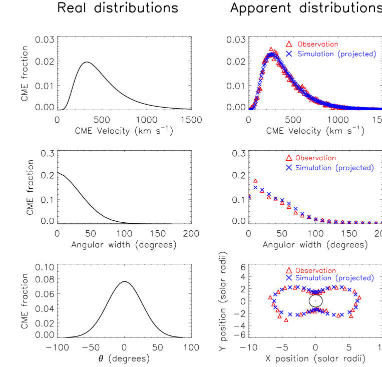
Figure 2: left column: The derived real distributions of the CME velocity (top), the angular width (middle), and the latitude $\theta$ (bottom); Right column: The apparent distributions of the CME velocity (top), the angular width (middle), and the MPA (bottom), where the triangles correspond to the SOHO/LASCO observations, and the crosses to the projection of the real distributions.

In order to get the statistical results of the observations, we appeal for the NASA/CDAW CME catalog, which is based on SOHO/LASCO observations. There are 14120 CMEs from 1996 January 11 to 2009 February 28 in this catalog. Among these events, 106 CMEs, whose velocity can not be detected, and 396 full halo CMEs are excluded, by which we obtain a sample of 13618 CMEs. The distributions of their apparent velocity, apparent angular width, and MPA are showed in Figure 2, which can be fit with lognormal, Gaussian, and double Gaussian functions, respectively, as shown in Equations (1)-(3). The average apparent velocity of the whole sample is about 418 $\rm{km~{}s}^{-1}$, and the average apparent angular width is about $42.7^{\circ}$.

$$f(v)={\frac{1}{0.57\sqrt{2\pi}v}}\exp{[-\frac{(\ln{v}-5.85)^{2}}{2\times 0.57^{2}}]}$$ (1)

$$f(AW)=\frac{1}{60.7\sqrt{2\pi}}\exp[-\frac{AW^{2}}{2\times 60.7^{2}}]$$ (2)

$$f(MPA)=\frac{1}{30.5\sqrt{2\pi}}\exp[-\frac{(MPA-90)^{2}}{2\times 30.5^{2}}]+\frac{1}{30.5\sqrt{2\pi}}\exp[-\frac{(MPA-270)^{2}}{2\times 30.5^{2}}]+0.003$$ (3)

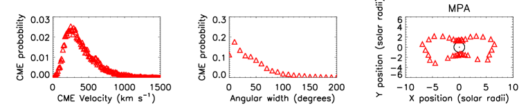
Figure 1: Distributions of the apparent velocity (left panel), the apparent angular width (middle panel), and the MPA (right panel) of the sample CMEs. The velocity is binned in 10 $\rm{km~{}s}^{-1}$intervals, the angular width is in $10^{\circ}$ intervals, and the MPA is in $10^{\circ}$ intervals. In the right panel, the distance of each triangle from the solar disk center represents the fraction of CMEs in this direction, and the circle marks the solar limb.

Since most CMEs propagate radially with an almost fixed angular width, the so-called cone model is often applied to describe the geometry of CMEs (Howard et al., 1982; Fisher et al., 1984; Michalek et al., 2003; Burkepile et al., 2004; Schwenn et al., 2005; Vršnak et al., 2007; Gao et al., 2009). With the assumption of the cone model, the kinematic properties of a CME in 3-dimensional space are characterized roughly by 4 variables, i.e., the real velocity ($v_{re}$), the real angular width ($AW_{re}$), the latitude ($\theta$) and the longitude ($\phi$) of the source center. It is reasonable to assume that CME sources are randomly distributed along the longitude in the heliocentric coordinates. For other three variables, we assume that the distributions of $v_{re}$, $AW_{re}$, and $\theta$ take the same functions as those of the apparent velocity, angular width, and the MPA (Equations 1-3), but with modified parameters, which are expressed as follows:

$$F(v_{re})=\frac{1}{v_{re}\sigma_{1}\sqrt{2\pi}}\exp[-\frac{(\ln{v_{re}}-\mu)^{2}}{2\sigma_{1}^{2}}],$$ (4)

$$F(AW_{re})=\frac{1}{\sigma_{2}\sqrt{2\pi}}\exp(-\frac{AW_{re}^{2}}{2\sigma_{2}^{2}}),$$ (5)

$$F(\theta)=\frac{1}{\sigma_{3}\sqrt{2\pi}}\exp(-\frac{\theta^{2}}{2\sigma_{3}^{2}}),$$ (6)

where $\mu$, $\sigma_{1}$, $\sigma_{2}$, and $\sigma_{3}$ are parameters to be determined.

In order to quantitatively calculate the projection effects on the CME velocity and angular width, we perform Monte Carlo simulations, which are described as follows: One million artificial CMEs are created, whose real velocity, angular width, and latitude of the central source region satisfy the distributions presented in Equations (4-6), and whose longitude of the central source region is randomly distributed in the range of $0^{\circ}$-$360^{\circ}$. Each of the artificial CMEs is then projected into the plane of the sky, through which the distributions of apparent velocity, apparent angular width, and the MPA can be derived. The four parameters ($\mu$, $\sigma_{1}$, $\sigma_{2}$, and $\sigma_{3}$) are adjusted until the projected distributions reproduce the observational counterparts (Equations 1-3), where the similarity is examined with the Kolmogorov test.

It is noted that, when projecting the artificial CMEs into the plane of the sky, the relation between the apparent velocity and the real value depends on the choice of the cone models (Schwenn et al., 2005; Vršnak et al., 2007; Gao et al., 2009). We assume that CMEs are symmetric, and propagate out radially through the corona, and their leading edge is a part of sphere, connecting the cone tangentially like an ice-cream, i.e., the Model C in Schwenn et al. (2005). Besides, according to Zhang et al. (2010), some CMEs, especially those near the Sun-Earth line, would be too faint to be detected by coronagraphs due to Thomson scattering, which should be taken into account in our study. For that purpose, we calculate the white-light intensity of each CME leading edge at $3R_{\odot}$ in the plane of the sky. Those CMEs whose white-light intensity falls below the $3\sigma$ of the fluctuation level of the solar wind are considered to be missed by coronagraphs (see Zhang et al., 2010, for details). The expression for calculating the Thomson-scattered intensity is given by Billings (1966). In our work we neglect the limb darkening effect, so the expression can be simplified as follows,

$$I=\pi\sigma J_{0}n_{0}R_{0}\frac{1}{81}\int^{\pi/2}_{0}(2C\cos^{3}\theta-A\cos^{5}\theta),$$ (7)

where $\sigma$ represents the Thomson scattering cross section, $J_{0}$ the photosphere radiative intensity at solar surface, $n_{0}$ the electron density, $R_{0}$ the solar radius, $\theta$ the angle between the plane of the sky and the direction of CME propagation, $A=\frac{\cos^{2}\theta\sqrt{9-\cos^{2}\theta}}{27}$, and $C=\frac{4}{3}-\frac{\sqrt{9-\cos^{2}\theta}}{3}-\frac{(9-\cos^{2}\theta)^{3/2}}{81}$.

3 Results

The derived real distributions of the CME velocity, the angular width, and the latitude are expressed as follows:

$$F(v_{re})=\frac{1}{0.53\sqrt{2\pi}v}\exp[-\frac{(\ln{v_{re}}-6.09)^{2}}{2\times 0.53^{2}}],$$ (8)

$$F(AW_{re})=\frac{1}{37.2\sqrt{2\pi}}\exp(-\frac{AW_{re}^{2}}{2\times 37.2^{2}}),$$ (9)

$$F(\theta)=\frac{1}{26.0\sqrt{2\pi}}\exp(-\frac{\theta^{2}}{2\times 26.0^{2}}).$$ (10)

Their profiles are depicted in the left column of Figure 3. As these quantities are projected into the plane of the sky, the resulting distributions of the apparent velocity, the angular width, and the MPA are shown in the right column of Figure 3 as crosses, where they are compared to the LASCO observations (triangles). It is seen that the simulated apparent distributions of the CME velocity, the angular width, and the MPA match the observations very well, which implies that the derived distributions in Equations (8–10) might well represent the real situation.

According to the derived real distributions of the CME velocity and the angular width ($AW_{re}$) for all non-full-halo CMEs, the average CME velocity is 514 $\rm{km~{}s}^{-1}$, which is $\sim 23\%$ larger than the apparent value, and the average angular width is $33^{\circ}$, which is $\sim 23\%$ smaller than the apparent value. In particular, for those CMEs whose angular widths are between $20^{\circ}$ and $120^{\circ}$ (the so-called normal CMEs in Yashiro et al., 2004), the corrected average CME velocity is 510 $\rm{km~{}s}^{-1}$, which is $\sim 30\%$ larger than the apparent value (392 $\rm{km~{}s}^{-1}$), and the corrected average angular width is $43.4^{\circ}$, which is $\sim 17\%$ smaller than the apparent value ($52^{\circ}$).

It is noticed that the real angular width distribution is peaked near $0^{\circ}$, however, its apparent angular width is peaked around $10^{\circ}$, which is consistent with the observations. Our simulations reveal that the significant drop of the number of narrow CMEs (with the angular width less than $10^{\circ}$) is due to that some of them are two weak to be detected when they propagate not far from the Sun-Earth direction.

4 Discussions

The accumulating observations of CMEs enable the statistics of their properties, such as their angular size and their kinematics. However, the measurements of the CME geometry and kinematics suffer from the projection effects, and it is expected that the real angular width should be smaller, whereas the real velocity should be larger. In this paper, with a forward modeling by Monte Carlo simulations, we corrected the distributions of the CME velocity and the angular width for the projection effects, as revealed by Equations (8–10). It is found that (1) for all non-full-halo CMEs, the real velocity is averaged at 514 $\rm{km~{}s}^{-1}$, and the real angular width is averaged at $33^{\circ}$, in contrast to 418 $\rm{km~{}s}^{-1}$and 42.7^∘ before correction; (2) for CMEs with the apparent angular width between $20^{\circ}-120^{\circ}$, the real velocity is averaged at 510 $\rm{km~{}s}^{-1}$, and the real angular width is averaged at $43.4^{\circ}$, in contrast to 392 $\rm{km~{}s}^{-1}$and 52^∘ before correction. The average real velocity of CMEs derived in this paper is similar to that of the limb events, which are free of the projection effects (Burkepile et al., 2004).

It should be noted that in our forward modeling, it was assumed for simplicity that the three prescribed variables (i.e., the CME velocity, the angular width, and the latitude of the central source region) are completely independent. With a large sample, Yeh et al. (2005) did find that there is little correlation between the CME velocity and the angular width. However, Yashiro et al. (2004) and Vršnak et al. (2007) claimed that wider CMEs tend to be faster. In order to clarify the discrepancy, we collect the 13618 non-full-halo CME events observed by SOHO/LASCO during the period 1996 January - 2009 February and display the scatter plot of the relation between the observed CME angular width and the velocity in the left panel of Figure 4. It is found that the two quantities present a very weak positive correlation, with the correlation coefficient being only 0.23. We also divide the sample into a subsample with CMEs observed near solar maximum and another subsample with CMEs near solar minimum, it is also revealed that the CME velocity and the angular width present little correlation. For comparison, the right panel of Figure 4 displays the scatter plot of the CME velocities and the angular widths of the artificial CMEs in our Monte Carlo simulations. It can be seen that the distributions of the scatter points in the two panels of Figure 4 are quite similar. The linear Pearson correlation test indicates that the similarity between the two panels is as high as 0.95. It is noted that the sparse data points with $v>1000$ $\rm{km~{}s}^{-1}$or $AW>120^{\circ}$ are not shown in Figure 4 in order to make the figure clear, though they are included in our study.

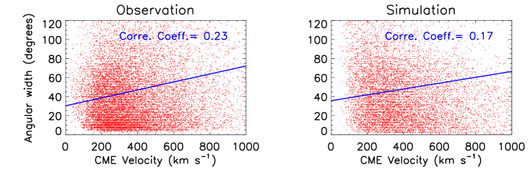
Figure 3: Scatter plots of the relation between the CME velocity and the angular width in observation (left) and simulation (right). The solid lines represent the linearly fitted lines.

In Figure 4 we compare the correlations between the CME velocity and the MPA in both observations and simulations. The left panel displays the scatter plot in the observations, where we can see that the correlation coefficient between the CME velocity and the MPA is almost zero. The right panel shows the corresponding scatter plot in our Monte Carlo simulations. The linear Pearson correlation test indicates that the similarity between the distributions in the two panels is as high as 0.91. Similarly to Figure 4, the sparse data points with $v>1000$ $\rm{km~{}s}^{-1}$or $MPA>200^{\circ}$ are not shown in Figure 4, though they are included in our study.

Figure 4: Scatter plots of the relation between the CME velocity and the MPA in observation (left) and simulation (right). The solid lines represent the linearly fitted lines.

It is noted in passing that the CME angular width and the MPA also show little correlation. Therefore, with the largest-ever sample that includes almost all the CMEs observed by the SOHO/LASCO coronagraph, we found that the CME velocity, the CME angular width, and the latitude of the central source region are all mutually uncorrelated. Such a lack of correlation validates our assumptions used in our forward modeling in deriving the CME real velocity and angular width distributions.