SPECTRAL STATISTICS OF “CELLULAR” BILLIARDS

Abstract.

For a bounded domain $\Omega^{0}\subset\mathbb{R}^{2}$ whose boundary contains a number of flat pieces $\Gamma_{i}$, $i=1,\dots l$ we consider a family of non-symmetric billiards $\Omega$ constructed by patching several copies of $\Omega^{0}$ along $\Gamma_{i}$’s. It is demonstrated that the length spectrum of the periodic orbits in $\Omega$ is degenerate with the multiplicities determined by a matrix group $G$. We study the energy spectrum of the corresponding quantum billiard problem in $\Omega$ and show that it can be split in a number of uncorrelated subspectra corresponding to a set of irreducible representations $\alpha$ of $G$. Assuming that the classical dynamics in $\Omega^{0}$ are chaotic, we derive a semiclassical trace formula for each spectral component and show that their energy level statistics are the same as in standard Random Matrix ensembles. Depending on whether ${\alpha}$ is real, pseudo-real or complex, the spectrum has either Gaussian Orthogonal, Gaussian Symplectic or Gaussian Unitary types of statistics, respectively.

1. Introduction

According to the Bohigas-Giannoni-Schmit conjecture [1] the energy spectrum of a generic Hamiltonian system with classically chaotic dynamics is distributed in the same way as spectra of the standard random matrix ensembles within the same symmetry class. In particular, the spectral statistics of spinless single-particle systems with time-reversal invariant classical chaotic dynamics can usually be described by the Gaussian Orthogonal Ensemble (GOE), or by the Gaussian Unitary Ensemble (GUE), if the time-reversal invariance is broken. For chaotic single-particle systems with half-integer spin the spectral statistics are typically the same as in the Gaussian Symplectic Ensemble (GSE). There exist, however, a few notable exceptions from this rule. It is known, for instance, that the presence of additional symmetries might lead to a change of the spectral statistics [2, 3]. If the system possesses a discreate symmetry group $H$, its spectrum can be split into a number of uncorrelated subspectra, where each spectral component corresponds to an irreducible representation $\alpha$ of $H$ [4, 5]. The distribution of the energy levels $\{E^{(\alpha)}_{n}\}$ within each sector depends then on the type of the representation $\alpha$ [6, 7]. For real and pseudo-real representations the corresponding spectral statistics are of GOE and of GSE type, respectively. If, on the other hand, $\alpha$ is complex, then the corresponding spectral statistics are of GUE type. As a result, even time-reversal invariant systems might contain subspectra of GUE type provided $H$ has complex irreducible representations [3, 6]. Other examples of non-standard spectral statistics are provided by the Laplacian eigenvalues of certain arithmetic surfaces of constant negative curvature [8, 9], as well as by some linear hyperbolic automorphisms of the 2-torus (cat maps) [10, 11]. Anomalous spectral statistics also appear in some chaotic systems with several ergodic components [12, 13].

From the semiclassical point of view deviations from the spectral universality can be always traced to a certain anomaly in the length spectrum of the classical periodic orbits (PO). For instance, additional geometrical symmetries imply degeneracies in the length spectrum of periodic orbits. Note, however, that even in the absence of geometrical symmetries degeneracies in the length spectrum might exist. This happens, for instance, in the case of arithmetic surfaces of negative curvature, where large multiplicities of the periodic orbits lead to the spectral statistics reminiscent of the Poissonian distribution. In the present work we consider another class of non-symmetric billiards whose length spectrum of periodic orbits is degenerate. These billiards are constructed in the following way. Let $\Omega^{0}$ be a bounded domain on $\mathbb{R}^{2}$ with the boundary $\partial\Omega^{0}$ containing $l$ flat pieces (i.e., line segments) $\Gamma_{i}$, $i=1,\dots l$. The billiard domain $\Omega$ is then builded up by taking $N$ copies of $\Omega^{0}$ and connecting them with the opposite orientations along $\Gamma_{i}$’s, see fig. 1a. The resulting domain $\Omega$ is equipped with the flat metric and in some cases with an appropriate choice of $\Omega^{0}$ can be embedded into $\mathbb{R}^{2}$. In what follows we will refer to any such domain $\Omega$ as cellular billiard and to $\Omega^{0}$ as fundamental cell. It should be noted that the same construction can be carried out in any dimension. In particular, starting from a one-dimensional fundamental cell one can also construct (quantum) cellular graphs, see fig. 1b. It is easy to see that the classical dynamics in $\Omega$ is intimately connected with the classical dynamics in $\Omega^{0}$. Specifically, for every periodic orbit in $\Omega$ there exists a corresponding periodic orbit in $\Omega^{0}$ of the same length. The opposite, however, is not always true: a periodic orbit in $\Omega^{0}$, in general, gives rise to a number (which can be also zero) of periodic orbits in $\Omega$. As a result, $\Omega^{0}$ and $\Omega$ posses the same length spectrum of periodic orbits but with different multiplicities, see fig. 1a.

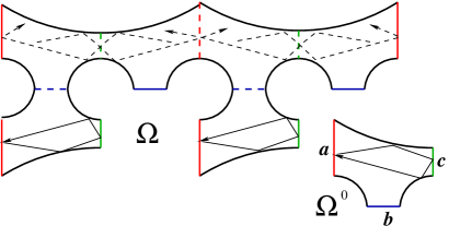
(a)  (b)

Figure 1. Construction of cellular (quantum) billiards (a) and (quantum) graphs (b). The billiard $\Omega$ is obtained by connecting six copies of $\Omega^{0}$ along its flat sides (coloured lines). At each flat part of the billiard boundary $\partial\Omega$ we impose either Dirichlet or Neumann boundary conditions.

Consider now the corresponding quantum billiard problem in $\Omega$:

(1.1) $$-\Delta_{\Omega}\varphi=\lambda\varphi,$$

where the function $\varphi$ satisfies some boundary conditions at $\partial\Omega$ and $\Delta_{\Omega}$ stands for the corresponding Laplacian. Note by passing, that the spectral problem for such billiards has previously attracted an attention in connection to the famous question of M. Katz [15]: “Can one hear the shape of a drum?”. It was shown [16] that starting from the same initial domain $\Omega^{0}$ one can construct in certain cases a pair of non-isometric domains $\Omega$, $\Omega^{\prime}$ such that the spectra of $\Delta_{\Omega}$ and $\Delta_{\Omega^{\prime}}$ coincide (for a similar construction of isospectral graphs, see [17, 18]). Here we are rather interested in the spectral properties of $\Delta_{\Omega}$ for a general cellular billiard $\Omega$. Note that, generically, $\Omega$ does not have geometric symmetries. On the other hand, the length spectrum of periodic orbits in $\Omega$ is degenerate and one might suspect that the energy levels statistics of $\Delta_{\Omega}$ exhibit an anomaly.

The main goal of this paper is to give a precise description of the spectral structure of $\Delta_{\Omega}$, based on the assumption of chaotic dynamics in the fundamental cell $\Omega^{0}$. As we will show, the situation here is reminiscent of that encountered in systems with geometrical symmetries. Namely, $\Delta_{\Omega}$ can be split in a number of subspectra:

(1.2) $$\Delta_{\Omega}=\bigoplus_{\alpha\in{\mathcal{R}}}\Delta^{(\alpha)}_{\Omega},$$

where the sum runs over a subset ${\mathcal{R}}$ of irreducible representations for certain matrix group $G$. Note that in general $G$ is not a symmetry group of the billiard domain, but rather a structure group which determines multiplicities of periodic orbits in $\Omega$. (The exact definition of $G$ and the relevant set ${\mathcal{R}}$ of its irreducible representations will be provided in the body of the paper.) As in the case of geometrical symmetries, the spectral statistics of each sector $\Delta^{(\alpha)}_{\Omega}$ turns out to be determined by the type of the representation $\alpha$ – the statistics are of GUE type, if the representation is complex and of GOE, GSE types, if the representation is real or pseudo-real, respectively. Furthermore, we show that the spectra of different sectors $\alpha$ are uncorrelated.

The paper is organised as follows. In Sec. 2 we consider the semiclassical trace formula for $\Delta_{\Omega}$ and express the multiplicities $\eta_{\gamma}$ of the periodic orbits $\gamma$ in $\Omega$ through the traces of certain class of permutation matrices. We then show that $\eta_{\gamma}$ combined with the phases (resulting from the Dirichlet boundary conditions) can be represented as characters of the standard representation for some matrix group $G$. In Sec. 3 we apply the trace formula to obtain spectral correlations of $\Delta_{\Omega}$. We show that the resulting spectral statistics are, in general, mixtures of GUE, GOE and GSE types of distributions. In Sec. 4 we demonstrate that the spectrum of $\Delta_{\Omega}$ can be split into a number of subspectra corresponding to irreducible representations of $G$ and derive a semiclassical trace formula for these subspectra in Sec. 5. Finally, the conclusion is presented in Sec. 6.

2. Semiclassical trace formula

Let $\Omega^{0}$ be a bounded domain on $\mathbb{R}^{2}$, with a piecewise smooth boundary $\partial\Omega^{0}$ containing $l$ flat pieces $\Gamma_{i}$, $i=1,\dots l$. We will consider the associated quantum Hamiltonian ${\widehat{H}}^{(0)}:=-(\hbar^{2}/2)\Delta_{\Omega^{0}}$, where $\hbar$ is Planck’s constant and $\Delta_{\Omega^{0}}$ is the Laplacian in $\Omega^{0}$ with the Neumann boundary conditions at $\partial\Omega^{0}$. The spectrum $\{E^{(0)}_{j}\}^{\infty}_{j=0}$, $E^{(0)}_{j}=\hbar^{2}\lambda^{(0)}_{j}/{2}$ of ${\widehat{H}}^{(0)}$ is then defined by the solutions of the following eigenvalue problem

(2.1) $$-\Delta\varphi^{(0)}_{j}=\lambda^{(0)}_{j}\varphi^{(0)}_{j},\qquad\varphi^{(0)}_{j}\in L^{2}(\Omega^{0}),\quad\partial_{n}\varphi^{(0)}_{j}|_{{\partial\Omega^{0}}}=0.$$

Now, take $\Omega^{0}$ as the fundamental cell and construct a cellular billiard $\Omega$ by means of the procedure described in the previous section. Note that, in general, the billiard boundary $\partial\Omega$ contains a number of flat pieces corresponding to unpaired sides $\Gamma_{i}$ of the copies of $\Omega^{0}$, see fig. 1. We will study the quantum billiard problem in $\Omega$ for mixed Dirichlet-Neumann boundary conditions at flat pieces of $\partial\Omega$. For the sake of concreteness we fix the Neumann boundary conditions at the rest of the boundary. Let $\partial\Omega_{i}$, $i=1,\dots\ell$ be the flat pieces of $\partial\Omega$ with the Dirichlet boundary conditions and let $\overline{\partial\Omega}=\partial\Omega\backslash\cup_{i}^{\ell}\partial\Omega_{i}$ be the remaining part of the boundary, then the eigenvalue problem

$$-\Delta\varphi_{j}=\lambda_{j}\varphi_{j}, \,\,\,\varphi_{j}\in L^{2}(\Omega),$$

(2.2) $$\varphi_{j}|_{\partial\Omega_{k}}=0,\,\,k=1,\dots\ell, \,\,\,\partial_{n}\varphi_{j}|_{\overline{\partial\Omega}}=0,$$

defines the Laplace operator $\Delta_{\Omega}$ and the energy levels $\{E_{j}\}^{\infty}_{j=0}$, $E_{j}=\hbar^{2}\lambda_{j}/2$ of the corresponding quantum Hamiltonian ${\widehat{H}}:=-(\hbar^{2}/2)\Delta_{\Omega}$. In what follows we will consider the spectral density functions for the quantum billiards in $\Omega^{0}$, $\Omega$:

(2.3) $$d^{(0)}(E)=\sum_{n=0}^{\infty}\delta(E-E^{(0)}_{n}),\qquad d(E)=\sum_{n=0}^{\infty}\delta(E-E_{n})$$

under the assumption that the classical dynamics in the fundamental cell $\Omega^{0}$ are chaotic.

The spectral function $d^{(0)}(E)=\bar{d}^{(0)}(E)+d^{(0)}_{\mathrm{osc}}(E)$ can be split into the smooth $\bar{d}^{(0)}(E)$ and the oscillating part whose semiclassical form is given by the Gutzwiller trace formula [19]:

(2.4) $$d^{(0)}_{\mathrm{osc}}(E)=\frac{1}{\pi\hbar}{\mathrm{Re}}\sum_{\gamma\in\mathrm{PPO(\Omega^{0})}}{\mathcal{A}}_{\gamma}\exp{\left(\frac{i}{\hbar}S_{\gamma}(E)\right)}+\Bigl{\{}\begin{subarray}{c}\text{Contribution from}\\ \text{repetition of p.o.}\end{subarray}\Bigr{\}}.$$

Here the sum runs over the set of all prime periodic orbits (PPO) in $\Omega^{0}$ and $S_{\gamma}$, ${\mathcal{A}}_{\gamma}$ are the action (including Maslov indices) and the stability factor of $\gamma$. In eq. (2.4) we singled out the contribution of the prime periodic orbits, as only these orbits are relevant for the spectral correlations. The contributions from the periodic orbits with a number of repetitions turn out to be suppressed by their large instability factors, see e.g., [19].

Analogously, one can express the spectral density of states for the billiard $\Omega$ in terms of its periodic orbits. Since each periodic orbit of $\Omega$ is also a periodic orbit of $\Omega^{0}$, the oscillating part of $d(E)=\bar{d}(E)+d_{\mathrm{osc}}(E)$ can be represented as a sum over the periodic orbits $\gamma$ of the billiard $\Omega^{0}$:

(2.5) $$d_{\mathrm{osc}}(E)=\frac{1}{\pi\hbar}{\mathrm{Re}}\sum_{\gamma\in\mathrm{PPO(\Omega^{0})}}\chi_{\gamma}{\mathcal{A}}_{\gamma}\exp{\left(\frac{i}{\hbar}S_{\gamma}(E)\right)}+\Bigl{\{}\begin{subarray}{c}\text{Contribution from}\\ \text{repetition of p.o.}\end{subarray}\Bigr{\}},$$

where $\chi_{\gamma}=(-1)^{k_{\gamma}}\eta_{\gamma}$ with $k_{\gamma}$ being the number of times $\gamma$ hits the pieces of the boundary with the Dirichlet boundary conditions and $\eta_{\gamma}\in\mathbb{Z}^{+}$ being the multiplicity of $\gamma$. Note that the forms of (2.4) and (2.5) are almost identical with a noticeable difference of additional multiplicity factors $\chi_{\gamma}$ in the last expression. Let us show now that these factors can be identified as characters of the standard representation for some matrix group.

Let $\{\Gamma_{k},k=1,\dots l\}$ be the set of flat components at the boundary of the domain $\Omega^{0}$. For each such component $\Gamma_{k}$ we define an associated $N\times N$ matrix $\sigma^{(k)}$ in the following way. Let $\Omega^{0}_{i}$, $i=1,\dots N$, be $N$ copies of $\Omega^{0}$ which compose the billiard $\Omega$. Then $\sigma^{(k)}_{i,j}=1$ for $i\neq j$ if $\Omega^{0}_{i}$ is connected to $\Omega^{0}_{j}$ through the side $\Gamma_{k}$, $\sigma^{(k)}_{i,i}=1$ (resp. $\sigma^{(k)}_{i,i}=-1$) if the boundary component $\Gamma_{k}$ of $\partial\Omega^{0}_{i}$ belongs to the boundary $\partial\Omega$ with the Neumann boundary conditions (resp. the Dirichlet boundary conditions) and $\sigma^{(k)}_{i,j}=0$, otherwise. The set of matrices $\{\sigma^{(k)},k=1,\dots l\}$ generates then the group $G$ with the multiplication operation given by the standart matrix product. In particular, for purely Neumann boundary conditions on $\partial\Omega$, $\sigma^{(k)}$ are just permutation matrices and $G$ is isomorphic to a subgroup of the permutation group of $N$ elements. Since $G$ is a matrix group, it admits the standard representation $\rho$, such that $\rho_{i,j}(\sigma)=\sigma_{i,j}$ for any $\sigma\in G$. It is straightforward to see that the multiplicity factors $\chi_{\gamma}$ can be expressed through the charactors of $\rho$. Given a periodic orbit $\gamma$ in $\Omega^{0}$, denote $\Gamma_{k_{1}}\Gamma_{k_{2}}\dots\Gamma_{k_{\bar{n}}}$, $k_{i}\in\{1,\dots l\}$ the (time) ordered sequence of flat pieces of $\partial\Omega^{0}$ in which the billiard ball flying along $\gamma$ hits the boundary, then

(2.6) $$\chi_{\gamma}={\mathrm{Tr}}{\sigma_{\gamma}},\qquad\sigma_{\gamma}=\prod_{i=1}^{\bar{n}}\sigma^{(k_{i})}\in G.$$

The above formula can be interpreted in the following way. Any periodic trajectory $\gamma$ in $\Omega^{0}$ passing through a point $x\in\Omega^{0}$ gives rise to $N$ trajectories $\{\gamma_{1},\dots\gamma_{N}\}$ in $\Omega$. Each trajectory $\gamma_{j}$ starts at the point $x_{j}$, where $x_{i}\in\Omega^{0}_{i}$, $i=1\dots N$ are the lifts of $x$ on $\Omega$. Since $\gamma$ starts and ends at the same point, the set of endpoints of $\gamma_{1},\dots\gamma_{N}$ is, in fact, a permutation of the initial points $\{x_{1},\dots x_{N}\}$. Specifically, $x_{j}$ is the end point of $\gamma_{i}$ if $(i,j)$’s element of $\sigma_{\gamma}$ is nonzero. As a result, by setting all nonvanishing elements of $\sigma_{\gamma}$ to $+1$ we obtain a permutation matrix of initial and final conditions, where the number of units at the diagonal defines the number of periodic trajectories among $\{\gamma_{1},\dots\gamma_{N}\}$. Furtheremore, having the elements of $\sigma^{(k)}$ with both negative and positive signs allows us to take in account different boundary conditions on $\partial\Omega$ which are relevant for the semiclassical trace formula.

As an example, let us consider two billiards shown in fig. 2 with the Dirichlet boundary conditions on the flat parts of the boundary $\partial\Omega$.

Example 2.1.

For the billiard in fig. 2a the generating matrices are given by

$$\sigma_{a}=\begin{pmatrix}-1&0&0\\ 0&0&1\\ 0&1&0\end{pmatrix},\quad\sigma_{b}=\begin{pmatrix}0&1&0\\ 1&0&0\\ 0&0&-1\end{pmatrix},\quad\sigma_{c}=\begin{pmatrix}-1&0&0\\ 0&-1&0\\ 0&0&-1\end{pmatrix}.$$

The group generated by $\sigma_{a},\sigma_{b},\sigma_{c}$ contains $10$ elements: $G=\{\sigma_{0}\sigma,\sigma_{1}\sigma|\sigma\in G_{0}\}$, where

$$\sigma_{0}=-\sigma_{1}=\begin{pmatrix}1&0&0\\ 0&1&0\\ 0&0&1\end{pmatrix}\quad\mbox{ and }G_{0}=\{\sigma_{0},\sigma_{a},\sigma_{b},\sigma_{a}\sigma_{b},\sigma_{b}\sigma_{a}\}.$$

Note also that $G_{0}$ is isomorphic to the group of permutations of three elements.

For the billiard shown in fig. 2b there is an additional connection between first and third copies of the fundamental cell and the generators of the group $G$ are given by:

$$\sigma_{a}=\begin{pmatrix}-1&0&0\\ 0&0&1\\ 0&1&0\end{pmatrix},\quad\sigma_{b}=\begin{pmatrix}0&1&0\\ 1&0&0\\ 0&0&-1\end{pmatrix},\quad\sigma_{c}=\begin{pmatrix}0&0&1\\ 0&-1&0\\ 1&0&0\end{pmatrix},$$

and $G=\{\sigma_{i}\sigma|i=0,1,2,3;\sigma\in G_{0}\}$, where $G_{0}$ is defined as above, with

$$\sigma_{0}=\begin{pmatrix}1&0&0\\ 0&1&0\\ 0&0&1\end{pmatrix},\sigma_{1}=\begin{pmatrix}1&0&0\\ 0&-1&0\\ 0&0&-1\end{pmatrix},\sigma_{2}=\begin{pmatrix}-1&0&0\\ 0&-1&0\\ 0&0&1\end{pmatrix},\sigma_{3}=\begin{pmatrix}-1&0&0\\ 0&1&0\\ 0&0&-1\end{pmatrix}.$$

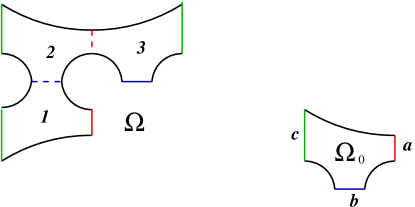
(a)          (b)

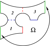
Figure 2. Pictures of two billiards considered in Example 2.1. Note that in the second case the first and the third copy of $\Omega_{0}$ are connected along the flat pieces of the boundary (marked by green colour), as shown by the arrow.

3. Spectral correlations

We now proceed with the calculations of the form factor

$$K(\tau)=\int_{-\infty}^{+\infty}R(x/\bar{d})e^{-2\pi i\tau x}dx$$

for the two-point correlation function of the spectral level density:

(3.1) $$R(\varepsilon)=\frac{1}{\bar{d}^{2}}\left\langle d\left(E+\frac{\varepsilon}{2}\right)d\left(E-\frac{\varepsilon}{2}\right)\right\rangle_{E}-1.$$

Using the semiclassical expression (2.5) for the density of states and expanding the actions $S(E\pm\frac{\varepsilon}{2})\approx S(E)\pm\frac{\varepsilon}{2}T(E)$ up to the linear term one obtains

(3.2) $$K(\tau)=\frac{1}{T_{\scriptscriptstyle\mathrm{H}}^{2}}\left\langle\sum_{\gamma,\gamma^{\prime}}\chi_{\gamma}\chi_{\gamma^{\prime}}{\mathcal{A}}_{\gamma}{\mathcal{A}}^{*}_{\gamma^{\prime}}\exp{\left(\frac{i}{\hbar}(S_{\gamma}-S_{\gamma^{\prime}})\right)}\delta\left(\tau-\frac{(T_{\gamma}+T_{\gamma^{\prime}})}{2T_{\scriptscriptstyle\mathrm{H}}}\right)\right\rangle_{E},$$

where $T_{\gamma},T_{\gamma^{\prime}}$ stand for periods of $\gamma,\gamma^{\prime}\in\mathrm{PPO(\Omega^{0})}$, and $T_{\scriptscriptstyle\mathrm{H}}=2\pi\hbar\bar{d}$ is the Heisenberg time for $\Omega$. Note that the spectral form factor $K_{0}(\tau)$ of the quantum billiard in $\Omega^{0}$ can be expressed in a similar way by setting all multiplicity factors $\chi_{\gamma},\chi_{\gamma^{\prime}}$ in eq. (3.2) to one and rescaling $T_{\scriptscriptstyle\mathrm{H}}$ by the factor $1/N$:

(3.3) $$K_{0}(\tau)=\frac{N^{2}}{T_{\scriptscriptstyle\mathrm{H}}^{2}}\left\langle\sum_{\gamma,\gamma^{\prime}}{\mathcal{A}}_{\gamma}{\mathcal{A}}^{*}_{\gamma^{\prime}}\exp{\left(\frac{i}{\hbar}(S_{\gamma}-S_{\gamma^{\prime}})\right)}\delta\left(\tau-\frac{(T_{\gamma}+T_{\gamma^{\prime}})}{2T_{\scriptscriptstyle\mathrm{H}}/N}\right)\right\rangle_{E}.$$

In what follows we are going to establish connection between $K_{0}(\tau)$ and $K(\tau)$.

The semiclassical expressions (3.2,3.3) can be used in order to calculate $K(\tau)$, $K_{0}(\tau)$ perturbatively, as functions of the parameter $\tau$. The leading order $\tau^{1}$ contribution can be obtained using so-called diagonal approximation, where only pairs of the same periodic orbits are considered [14]. The next order $\tau^{2}$ term is due to the contribution of pairs of periodic orbits with one selfencounter (Sieber-Richter pairs) [20]. In the same spirit the higher order terms $\tau^{n+1}$ can be obtained from the correlations of non-identical trajectories with $n$ selfencounters [21]. Such correlating orbits can be organised into families according to their topological structure. Each family then, includes periodic orbits with close actions which systematically contribute into the sum. As a result, the form factor $K_{0}(\tau)$ can be written in the perturbative form as:

(3.4) $$K_{0}(\tau)=\sum^{\infty}_{n=1}\tau^{n}c_{n},\qquad c_{n}=\sum_{s\in{\mathcal{S}}_{n}}k_{n}^{(s)},$$

where the last sum runs over the set ${\mathcal{S}}_{n}$ of topologically different structures of periodic orbits having $n$ encounters. For generic form of the length spectrum of periodic orbits in chaotic systems with time reversal invariance, the contribution $k_{n}^{(s)}$ for each structure $s\in{\mathcal{S}}_{n}$ has been explicitly calculated in [21] and shown to reproduce RMT result:

$$\mathbf{GOE:}\,\,c_{1}=2,\,\,c_{n+1}=\frac{(-2)^{n}}{n},\,\,n\geq 1;\quad\mathbf{GUE:}\,\,c_{1}=1,\,\,c_{n+1}=0,\,\,n\geq 1;$$

$$\mathbf{GSE:}\,\,c_{1}=\frac{1}{2},\,\,c_{n+1}=\frac{1}{4n},\,\,n\geq 1.$$

To calculate the spectral form factor $K(\tau)$ for the billiard $\Omega$ we will assume that for long periodic trajectories the multiplicity factors $\chi_{\gamma}$ do not correlate with the actions $S_{\gamma}$. It follows then by (3.2) and (3.3) that

(3.5) $$K(\tau)=\frac{1}{N}\sum^{\infty}_{n=1}(N\tau)^{n}c^{\prime}_{n},\qquad c^{\prime}_{n}=\sum_{s\in{\mathcal{S}}_{n}}{\mathcal{D}}_{n}^{(s)}k_{n}^{(s)},$$

where $k_{n}^{(s)}$ are as in eq. (3.4), and

$${\mathcal{D}}_{n}^{(s)}=\left\langle\chi_{\gamma}\chi_{\gamma^{\prime}}\right\rangle_{s},$$

with the average over all periodic orbits $\gamma,\gamma^{\prime}$ having the same topological structure $s\in{\mathcal{S}}_{n}$ of encounters. Since $\chi_{\gamma}$, $\chi_{\gamma^{\prime}}$ are characters of two group elements $\sigma_{\gamma},\sigma_{\gamma^{\prime}}\in G$ the above average over periodic trajectories can be substituted with the average over the set $G^{(s)}=\{(\sigma,\bar{\sigma})\}$ of pairs $\sigma,\bar{\sigma}\in G$ compatible with the structure $s$ of correlating periodic orbits:

(3.6) $${\mathcal{D}}_{n}^{(s)}=\frac{1}{|G^{(s)}|}\sum_{\sigma,\sigma^{\prime}\in G^{(s)}}\chi(\sigma)\chi(\sigma^{\prime}),$$

where the normalisation factor $|G^{(s)}|$ is the number of pairs in $G^{(s)}$.

It follows from eq. (3.5) that, in order to evaluate $K(\tau)$ one only need to know the coefficients ${\mathcal{D}}_{n}^{(s)}$. Below we show how to calculate ${\mathcal{D}}_{n}^{(s)}$ for a given structure $s$ of the correlating periodic orbits.

3.1. Diagonal approximation

For the diagonal approximation the two trajectories $\gamma,\gamma^{\prime}$ coincide and we have: $G^{(s)}=\{(g,g)|\,g\in G\}$. This yields

(3.7) $${\mathcal{D}}_{1}=\frac{1}{|G|}\sum_{\sigma\in G}(\chi(\sigma))^{2},\qquad\chi(\sigma)={\mathrm{Tr}}\sigma.$$

By the group orthogonality theorem (see e.g., [22]) it follows then

(3.8) $${\mathcal{D}}_{1}=\sum_{\alpha\in{\mathcal{R}}(\rho)}n^{2}_{\alpha},$$

where $n_{\alpha}$ is the number of times the irreducible representation $\alpha$ enters into $\rho$. If $n_{\alpha}=1$ for each $\alpha$, then ${\mathcal{D}}_{1}$ is just the number of irreducible representations contained in $\rho$.

3.2. Non-diagonal contribution

The second order term in eq. (3.5) comes from the correlations of periodic orbits shown in fig. 3. These periodic orbits can be represented as unions of two (directed) stretches: $a\cup b$, $a^{\prime}\cup b^{\prime}$, where $a$ is connected with $b$ (resp. $a^{\prime}$ with $b^{\prime}$) at the encounter region. Note that in the configuration space $a$ and $a^{\prime}$ are running close to each other. The same holds true for the stretches $b$ and $b^{\prime}$ which have, however, opposite orientations. Schematically, it is convenient to denote such correlating periodic orbits as $\gamma=ab$, $\gamma^{\prime}=a\bar{b}$, where the “bar” symbol stands for an “opposite orientation”. Such structure of $\gamma$, $\gamma^{\prime}$ implies that the pairs of group elements $(\sigma_{\gamma},\sigma_{\gamma^{\prime}})\in G^{(s)}$ in eq. (3.6) can be represented in the following form:

(3.9) $$\sigma_{\gamma}=gh,\qquad\sigma_{\gamma^{\prime}}=gh^{-1},$$

where $g$, $h$ correspond to the stretches $a$ and $b$, respectively. It is, therefore, necessary to calculate the following group average:

(3.10) $${\mathcal{D}}_{2}=\frac{1}{|G|^{2}}\sum_{h\in G}\sum_{g\in G}\chi(gh)\chi(gh^{-1}).$$

This quantity can be easily evaluated using the group orthogonality theorem.

(3.11) $${\mathcal{D}}_{2}=\frac{1}{|G|^{2}}\sum_{h,g\in G}\sum_{i,j,k=1}^{N}\sum_{\alpha,\beta\in{\mathcal{R}}(\rho)}\rho^{(\alpha)}_{i,j}(g)\rho^{(\alpha)}_{j,i}(h^{2})\rho^{(\beta)}_{k,k}(g)\\ =\frac{1}{|G|}\sum_{\alpha\in{\mathcal{R}}(\rho)}\frac{1}{m_{\alpha}}\sum_{h\in G}\chi^{(\alpha)}(h^{2})=\sum_{\alpha\in{\mathcal{R}_{\scriptscriptstyle\mathrm{r}}}(\rho)}\frac{n^{2}_{\alpha}}{m_{\alpha}}-\sum_{\beta\in{\mathcal{R}_{\scriptscriptstyle\mathrm{pr}}}(\rho)}\frac{n^{2}_{\beta}}{m_{\beta}},$$

where the indices in the last two sums run over the set of real ${\mathcal{R}_{\scriptscriptstyle\mathrm{r}}}(\rho)$ and pseudoreal ${\mathcal{R}_{\scriptscriptstyle\mathrm{pr}}}(\rho)$ irreducible representations entering $\rho$.

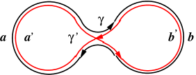
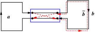
Figure 3. Sketch of a Sieber-Richter pair in configuration space (left) and the corresponding diagram (right). The two partner periodic orbits $\gamma=ab$, $\gamma^{\prime}=a\bar{b}$ depicted as solid (black) and dashed (red) lines follow each other at the stretch “$a$”, but after leaving the encounter region (shown as a (blue) rectangle on the right figure) move in the opposite directions at the stretches “$b$” and “$\bar{b}$”, respectively.

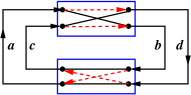
(a)          (b)

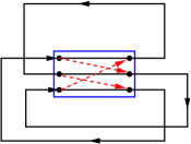
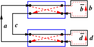
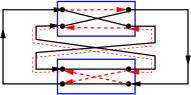
(c)      (d)      (e)

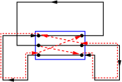
Figure 4. Five diagrams corresponding to topologically different families of correlating periodic orbits which contribute to the $\tau^{3}$ term of the form factor. The structures depicted at figures (c,d,e) appear only for systems with time reversal invariance.

To calculate $\tau^{3}$ term of $K(\tau)$ one needs to take in account several different structures of the correlating orbits, which are shown in fig. 4. In general all such structures can be separated into two categories: structures which are relevant both for systems with and without time reversal invariance and structures which are relevant only when time reversal invariance is present. The first category is composed of two “uni-directional” structures shown in figs. 4a,b. Here all correlating trajectories have the same direction at each of the encounters. The second category is represented by three “bi-directional” structures shown in figs. 4c,d,e, where correlating trajectories have different directions at least in one of the encounters. As we show bellow, the expression for ${\mathcal{D}}_{3}^{(s)}$ essentially depends on the type of the structure $s$. Let us consider for example the “bi-directional” diagram shown in fig. 4c. In that case the two correlating orbits have the structure $\gamma=abcd$ and $\bar{\gamma}=a\bar{d}c\bar{b}$, respectively. As before, we can use the group orthogonality theorem:

(3.12) $${\mathcal{D}}^{(c)}_{3}=\frac{1}{|G|^{4}}\sum_{g,h\in G}\sum_{f,e\in G}\chi(gfhe)\chi(ge^{-1}hf^{-1})\\ =\frac{1}{|G|^{3}}\sum_{g,h,f\in G}\sum_{\alpha\in{\mathcal{R}}(\rho)}\frac{n^{2}_{\alpha}}{m_{\alpha}}\chi^{(\alpha)}(g^{2}fh^{2}f^{-1})\\ =\frac{1}{|G|^{2}}\sum_{\alpha\in{\mathcal{R}}(\rho)}\frac{n^{2}_{\alpha}}{m^{2}_{\alpha}}\sum_{g,h\in G}\chi^{(\alpha)}(g^{2})\chi^{(\alpha)}(h^{2})=\sum_{\alpha\in{\mathcal{R}_{\scriptscriptstyle\mathrm{r}}}(\rho)}\frac{n^{2}_{\alpha}}{m^{2}_{\alpha}}+\sum_{\beta\in{\mathcal{R}_{\scriptscriptstyle\mathrm{pr}}}(\rho)}\frac{n^{2}_{\beta}}{m^{2}_{\beta}}.$$

It is straightforward to see that the same result holds for all “bi-directional” diagrams of order $\tau^{3}$, i.e., ${\mathcal{D}}^{(c)}_{3}={\mathcal{D}}^{(d)}_{3}={\mathcal{D}}^{(e)}_{3}$. On the other hand, for the “uni-directional“ diagram in fig. 4a one has $\gamma=abcd$ and $\bar{\gamma}=adcb$. This leads to

(3.13) $${\mathcal{D}}^{(a)}_{3}=\frac{1}{|G|^{4}}\sum_{g,h\in G}\sum_{f,e\in G}\chi(gfhe)\chi(gehf)\\ =\frac{1}{|G|^{4}}\sum_{g,h\in G}\sum_{f,e\in G}\chi(gfhe)\chi(f^{-1}h^{-1}e^{-1}g^{-1})=\sum_{\alpha\in{\mathcal{R}}(\rho)}\frac{n^{2}_{\alpha}}{m^{2}_{\alpha}}.$$

The same result ${\mathcal{D}}^{(a)}_{3}={\mathcal{D}}^{(b)}_{3}$ holds for the diagram on fig. 4b. Note that both expressions (3.12,3.13) have the same form with the notable difference of the range of irreducible representations $\alpha$ appearing there. Namely, the sum in eq. (3.13) runs only over real and pseudoreal irreducible representations entering $\rho$ while the sum in eq. (3.12) includes complex irreducible representations, as well.

Furtheremore, using the same approach it is straightforward to see that, for a general diagram of order $\tau^{n}$ the corresponding coefficients ${\mathcal{D}}^{(s)}_{n}$ are given by

(3.14) $${\mathcal{D}}^{\mathrm{uni}}_{n}=\sum_{\alpha\in{\mathcal{R}}(\rho)}\frac{n^{2}_{\alpha}}{m^{n-1}_{\alpha}},\qquad{\mathcal{D}}^{\mathrm{bi}}_{n}=\sum_{\alpha\in{\mathcal{R}_{\scriptscriptstyle\mathrm{r}}}(\rho)}\frac{n^{2}_{\alpha}}{m^{n-1}_{\alpha}}+\sum_{\beta\in{\mathcal{R}_{\scriptscriptstyle\mathrm{pr}}}(\rho)}\frac{n^{2}_{\beta}}{(-m_{\beta})^{n-1}},$$

for diagrams with “uni-directional” and “bi-directional” structures, respectively. Substituting (3.14) into eq. (3.5) and taking into account that $K_{0}(\tau)=K_{\scriptscriptstyle\mathrm{GOE}}(\tau)$ for a generic $\Omega^{0}$ with chaotic dynamics, we obtain:

(3.15) $$K(\tau)=\sum_{\alpha\in{\mathcal{R}_{\scriptscriptstyle\mathrm{r}}}(\rho)}n^{2}_{\alpha}\left(\frac{m_{\alpha}}{N}\right)K_{\scriptscriptstyle\mathrm{GOE}}\left(\frac{N}{m_{\alpha}}\tau\right)\\ +\sum_{\beta\in{\mathcal{R}_{\scriptscriptstyle\mathrm{pr}}}(\rho)}(2n_{\beta})^{2}\left(\frac{m_{\beta}}{2N}\right)K_{\scriptscriptstyle\mathrm{GSE}}\left(\frac{2N}{m_{\beta}}\tau\right)+\sum_{\nu\in{\mathcal{R}_{\scriptscriptstyle\mathrm{c}}}(\rho)}2n^{2}_{\nu}\tau.$$

Note, that since $\rho_{i,j}(g)$ are real matrices, for every complex representation $\nu$ entering $\rho$ the corresponding complex conjugate representation $\bar{\nu}$ enters $\rho$, as well. As a result, the last sum in (3.15) can be cast into the form

(3.16) $$\sum_{(\nu,\bar{\nu})\in{\mathcal{R}_{\scriptscriptstyle\mathrm{c}}}(\rho)}(2n_{\nu})^{2}\left(\frac{m_{\nu}}{N}\right)K_{\scriptscriptstyle\mathrm{GUE}}\left(\frac{N}{m_{\nu}}\tau\right),$$

where the sum runs over pairs of all complex representations and their conjugate counterparts. Eqs. (3.15, 3.16) suggest the following spectral structure of $\Delta_{\Omega}$:

Proposition 3.1.

Let $\rho$ be the standard representation of the structural group $G$ (as defined in Sec. 2) and let

$$\rho=\bigoplus_{\alpha\in{\mathcal{R}_{\scriptscriptstyle\mathrm{r}}}(\rho)}[\alpha]\bigoplus_{\beta\in{\mathcal{R}_{\scriptscriptstyle\mathrm{pr}}}(\rho)}[\beta]\bigoplus_{\nu\in{\mathcal{R}_{\scriptscriptstyle\mathrm{c}}}(\rho)}[\nu],$$

be its decomposition into a number of real, pseudoreal and complex irreducible representations. Then the spectrum of $\Delta_{\Omega}$ can be split accordingly:

i) For each real representation $\alpha$ entering $n_{\alpha}$ times $\rho$ there exists an associated GOE-like subspectrum with the density $\bar{d}_{\alpha}=\bar{d}\left(\frac{m_{\alpha}}{N}\right)$ and the number of degenerate levels $n_{\alpha}$.

ii) For each pseudoreal representation $\beta$ entering $n_{\beta}$ times $\rho$ there exists an associated GSE-like subspectrum with the dencity $\bar{d}_{\beta}=\bar{d}\left(\frac{m_{\beta}}{2N}\right)$ and the number of degenerate levels $2n_{\beta}$.

iii) For each pair of complex conjugate representations $(\nu,\bar{\nu})$ entering $n_{\nu}$ times $\rho$ there exists an associated GUE-like subspectrum with the density of levels $\bar{d}_{\nu}=\bar{d}\left(\frac{m_{\nu}}{N}\right)$ and the number of degenerate levels $2n_{\nu}$.

In the next section we analyse the origin of this spectral decomposition in cellular billiards.

4. Spectral decomposition

Before turning to the general case, let us consider, as an example, the billiards shown in fig. 2. By eq. (3.7) the leading order term of the form factor can be straightforwardly evaluated giving ${\mathcal{D}}_{1}=2$, ${\mathcal{D}}_{1}=1$ for the billiards in fig. 2a and fig. 2b, respectively. This can be understood, as an indication that the spectrum of the first billiard is composed of two independent GOE components, while the spectrum of the second billiard has a single GOE component. As we show below, this is indeed so, since for the billiard in fig. 2a it is actually possible to find a projection operator $P$ commuting with $\Delta_{\Omega}$. To construct such an operator, consider a continuous function $\psi\in C^{2}(\Omega)$ on $\Omega$ satisfying the same boundary conditions as in (2.2). Let $\{\psi_{1},\psi_{2},\psi_{3}\}$ be the restrictions of $\psi$ on $\Omega_{i},i=1,2,3$. Regarding $(\psi_{1},\psi_{2},\psi_{3})$ as the components of the three-dimensional vector, define the new set of functions $\{\psi^{\prime}_{1},\psi^{\prime}_{2},\psi^{\prime}_{3}\}$ on $\Omega_{i},i=1,2,3$:

(4.1) $$\psi^{\prime}_{i}=\sum_{j=1}^{3}p_{ij}\psi_{j},\qquad p=\frac{1}{3}\begin{pmatrix}-1&1&-1\\ 1&-1&1\\ -1&1&-1\end{pmatrix}.$$

We can now lift $\{\psi^{\prime}_{1},\psi^{\prime}_{2},\psi^{\prime}_{3}\}$ to the new function $\psi^{\prime}$ on $\Omega$, whose restrictions on $\Omega_{i},i=1,2,3$ are given by $\psi^{\prime}_{i}$’s. It is easy to see that $\psi^{\prime}$ is, in fact, continuous function on $\Omega$ satisfies the same boundary conditions as $\psi$. As a result, the map $P:\psi\to\psi^{\prime}$ defines the linear operator $P$ which acts on the domain $\mathrm{Dom}(\Delta_{\Omega})$ of $\Delta_{\Omega}$. Since any solution of eq. (2.2) is mapped by $P$ into another solution of this equation we have $[P,\Delta_{\Omega}]=0$. Furthermore, the property $p^{2}=p$ implies that $P$ is the projection i.e., $P^{2}=P$.

Turning now to the general case, for each representation $\alpha\in{\mathcal{R}}(\rho)$ entering $\rho$ define the following $N\times N$ matrix:

(4.2) $$p^{(\alpha)}=\frac{m_{\alpha}}{|G|}\sum_{\sigma\in G}\chi^{(\alpha)}(\sigma)\rho^{*}(\sigma).$$

By the group orthogonality theorem these matrices satisfy $p^{(\alpha)}p^{(\beta)}=p^{(\alpha)}\delta_{\alpha,\beta}$, for ${\alpha},\beta\in{\mathcal{R}}(\rho)$ and $\sum_{\alpha\in{\mathcal{R}}(\rho)}p^{(\alpha)}=1_{N\times N}$. Furthermore, it is straightforward to check that the projections (4.2) commute with $\rho(\sigma)$ for all $\sigma\in G$:

$$[p^{(\alpha)},\rho(\sigma)]=0,\quad{\alpha}\in{\mathcal{R}}(\rho).$$

We can now use $p^{(\alpha)}$’s in order to construct projection operators $P_{\alpha}$’s commuting with $\Delta_{\Omega}$. For a given state $\psi\in{\mathcal{H}}:=\mathrm{Dom}(\Delta_{\Omega})$, with the restrictions $\{\psi_{1},\dots\psi_{N}\}$ on $\Omega_{i}$, $i=1,\dots N$ let $\psi^{\prime}\in{\mathcal{H}}$ be the state whose restrictions on $\Omega_{i}$, $i=1,\dots N$ are given by

(4.3) $$\psi^{\prime}_{i}=\sum_{j=1}^{N}p^{(\alpha)}_{i,j}\psi_{j}.$$

With each $p^{(\alpha)}$ we associate the linear operation $P_{\alpha}$ which maps $\psi$ into $\psi^{\prime}$. It follows from the definition of $P_{\alpha}$ and the corresponding properties of $p^{(\alpha)}$ that $P_{\alpha}P_{\beta}=P_{\alpha}\delta_{\alpha,\beta}$ for any $\alpha,\beta\in{\mathcal{R}}(\rho)$, $\sum_{\alpha\in{\mathcal{R}}(\rho)}P_{\alpha}=\mathsf{1}$ and

$$[P_{\alpha},\Delta_{\Omega}]=0,\qquad\alpha\in{\mathcal{R}}(\rho).$$

Using these projection operators we can now split $\Delta_{\Omega}$ into the direct sum

(4.4) $$\Delta_{\Omega}=\bigoplus_{\alpha\in{\mathcal{R}}(\rho)}\Delta_{\Omega}^{(\alpha)},\qquad\Delta_{\Omega}^{(\alpha)}:=P_{\alpha}\Delta_{\Omega}P_{\alpha},$$

where each $\Delta_{\Omega}^{(\alpha)}$ acts on the subspace ${\mathcal{H}}_{\alpha}=P_{\alpha}{\mathcal{H}}$, ${\mathcal{H}}=\bigoplus_{\alpha\in{\mathcal{R}}(\rho)}{\mathcal{H}}_{\alpha}$.

Now, let us analyse degeneracies in the spectrum of each $\Delta_{\Omega}^{(\alpha)}$. To this end note that if $\alpha$ enters $n_{\alpha}$ times into $\rho$, the projection $p^{(\alpha)}$ can be split further into the sum $p^{(\alpha)}=\sum_{i=1}^{n_{\alpha}}p^{(\alpha)}_{i}$, such that the subspaces $h_{i}^{(\alpha)}:=p_{i}^{(\alpha)}h$, $h\cong\mathbb{C}^{N}$, $i=1,\dots n_{\alpha}$ are orthogonal to each other and remain invariant under the action of $\rho$. Furtheremore, in this case there exists a group of unitary matrices $u^{(\alpha)}$ commuting with $\rho(g)$ for all $g\in G$ which mix different subspaces $h^{(\alpha)}_{i}$’s inside $h^{(\alpha)}=h^{(\alpha)}_{1}\oplus\dots\oplus h^{(\alpha)}_{n_{\alpha}}$, but leave every vector $v$ orthogonal to $h^{(\alpha)}$ intact: $u^{(\alpha)}v=v$. By using previous arguments, we can lift the matrices $p_{i}^{(\alpha)},u^{(\alpha)}$ to the linear operators $P_{i,\alpha},U_{\alpha}$ acting on the Hilbert space ${\mathcal{H}}$. From this follows immediately that the Hilbert space ${\mathcal{H}}_{\alpha}$ can be split into the direct sum ${\mathcal{H}}_{\alpha}=\bigoplus^{n_{\alpha}}_{i=1}{\mathcal{H}}_{i,\alpha}$, ${\mathcal{H}}_{i,\alpha}=P_{i,\alpha}{\mathcal{H}}$ , where $[P_{i,\alpha},\Delta_{\Omega}]=0$, $P_{i,\alpha}P_{j,\alpha}=\delta_{i,j}$, $i=1,\dots n_{\alpha}$ and there is a group of unitary operators $U_{\alpha}$, $[U_{\alpha},\Delta_{\Omega}]=0$ which mix different ${\mathcal{H}}_{i,\alpha}$ and leave states from ${\mathcal{H}}_{\alpha^{\prime}}$ intact if $\alpha^{\prime}\neq\alpha$. In its turn this implies that the spectrum of each $\Delta_{\Omega}^{(\alpha)}$ is at least $n_{\alpha}$ times degenerate.

Remark 4.1.

For any real representation $\alpha$, the degeneracy of the corresponding spectral component is given (generically) by the number of times $\alpha$ enters $\rho$. It follows, however, from Proposition 3.1 that for complex and pseudoreal representations there should be additional double degeneracies in the spectrum. Indeed, for each pair of complex conjugate representations $(\nu,\bar{\nu})$ entering $\rho$, the set of eigenvectors of $\Delta_{\Omega}^{(\nu)}$ is mapped into the set of orthogonal eigenvectors of $\Delta_{\Omega}^{(\bar{\nu})}$ (and vice versa) by the complex conjugation operation. Since all eigenvectors of $\Delta_{\Omega}$ can be chosen to be real, $\Delta_{\Omega}^{(\nu)}$ and $\Delta_{\Omega}^{(\bar{\nu})}$ must have the same spectrum. For every pseudoreal representation $\beta$, there exists a unitary operator $A$, such that $A\bar{A}=-1$, where $\bar{A}$ is the complex conjugate of $A$ and $\beta(g)=A\bar{\beta}(g)A^{-1}$ for any $g\in G$, see [22]. Combining $A$ with the complex conjugation operation $Cv=\bar{v}$ we obtain the antiunitary operator $t=AC$ satisfying $t^{2}=-1$ and commuting with $\beta(g)$ for all $g\in G$. In its turn, this induces the antiunitary operator $T$ acting on ${\mathcal{H}}$, such that $[\Delta_{\Omega}^{(\beta)},T]=0$ and $T^{2}=-1$. By the last property vectors $\psi$ and $T\psi$ must be orthogonal to each other for any $\psi\in{\mathcal{H}}$, which implies the double degeneracy of the spectrum of $\Delta_{\Omega}^{(\beta)}$ (Kramers’ degeneracy), see e.g., [19].

5. Trace formula for subspectra

By the decomposition (4.4) the whole spectrum of $\Delta_{\Omega}$ can be represented as the union of spectra of the operators $\Delta_{\Omega}^{(\alpha)}$:

(5.1) $${\mathrm{Spec}}(\Delta_{\Omega})=\bigcup_{\alpha\in{\mathcal{R}}(\rho)}{\mathrm{Spec}}(\Delta_{\Omega}^{(\alpha)}).$$

It is therefore of interest to obtain a semiclassical expression for the spectral density of each $\Delta_{\Omega}^{(\alpha)}$ individually:

(5.2) $$d^{(\alpha)}(E)=-\frac{1}{\pi}{\mathrm{Im}}{\mathrm{Tr}}\left(P_{\alpha}\frac{1}{E+i\varepsilon-\Delta_{\Omega}}\right).$$

To this end we can use the same approach, as in the case of systems with geometric symmetries [4]. The starting point here is the following representation of the projected Green’s function:

(5.3) $${\mathbf{G}}_{\alpha}(E,x,x):=\left\langle x\left|P_{\alpha}\frac{1}{E+i\varepsilon-\Delta_{\Omega}}\right|x\right\rangle=\int_{\Omega}dy\,\left\langle y|\,P_{\alpha}\,|x\right\rangle{\mathbf{G}}(E,x,y),$$

where ${\mathbf{G}}(E,x,y)$ stands for the Green’s function in the billiard $\Omega$. Let $x^{(k)}$ denote the mirror image of the point $x$ in the domain $\Omega^{(k)}$, $k=1,\dots N$ with $x$ being equal to $x^{(m)}\in\Omega^{(m)}$, for some $m$. Using then the definition (4.2) we obtain from eq. (5.3)

(5.4) $${\mathbf{G}}_{\alpha}(E,x,x)=\sum_{k=1}^{N}p^{(\alpha)}_{k,m}{\mathbf{G}}(E,x^{(m)},x^{(k)})\\ =\frac{m_{\alpha}}{|G|}\sum_{\sigma\in G}\chi^{(\alpha)}(\sigma)\sum_{k=1}^{N}\rho_{k,m}^{*}(\sigma){\mathbf{G}}(E,x^{(m)},x^{(k)}).$$

In order to calculate the oscillating part $d_{{\mathrm{osc}}}^{(\alpha)}$ of the spectral density

(5.5) $$d^{(\alpha)}(E)=\bar{d}^{(\alpha)}(E)+d_{{\mathrm{osc}}}^{(\alpha)}(E)=-\frac{1}{\pi}{\mathrm{Im}}\int_{\Omega}dx\,{\mathbf{G}}_{\alpha}(E,x,x),$$

we can now use the standard semiclassical representation for the Green’s function ${\mathbf{G}}$ (see e.g., [19]):

(5.6) $${\mathbf{G}}_{{\mathrm{sc}}}(E,x^{(m)},x^{(k)})=\frac{1}{i\hbar}\sum_{\tilde{\gamma}[x^{(m)}\to x^{(k)}]}A_{\tilde{\gamma}}\exp{\left(\frac{i}{\hbar}S_{\tilde{\gamma}}(E)\right)},$$

where the sum runs over trajectories in $\Omega$ connecting $x^{(m)}$ to $x^{(k)}$, and $A_{\tilde{\gamma}}$, $S_{\tilde{\gamma}}$ stand for their stability factors and actions, respectively. Note that the above expression can be also rewritten as a sum over closed trajectories $\gamma[x\to x]$ in the billiard $\Omega^{0}$:

(5.7) $${\mathbf{G}}_{{\mathrm{sc}}}(E,x^{(m)},x^{(k)})=\frac{1}{i\hbar}\sum_{\gamma[x\to x]}\rho_{m,k}(\sigma_{\gamma})A_{\gamma}\exp{\left(\frac{i}{\hbar}S_{\gamma}(E)\right)},$$

with $\sigma_{\gamma}$ being the permutation matrix (2.6) corresponding to the trajectory $\gamma$. Substituting now (5.7) into (5.4) and performing saddle point approximation in eq. (5.5) we obtain for the oscillating part of the spectral density:

(5.8) $$d_{{\mathrm{osc}}}^{(\alpha)}(E)=\frac{m_{\alpha}}{\pi\hbar|G|}{\mathrm{Re}}\left\{\sum_{\sigma}\sum_{\gamma\in\mathrm{PO(\Omega^{0})}}\chi^{(\alpha)}(\sigma)\chi(\sigma^{-1}\sigma_{\gamma}){\mathcal{A}}_{\gamma}\exp{\left(\frac{i}{\hbar}S_{\gamma}(E)\right)}\right\}.$$

Using the group orthogonality theorem we can perform summation over $\sigma$ and finally get

(5.9) $$d_{{\mathrm{osc}}}^{(\alpha)}(E)=\frac{n_{\alpha}}{\pi\hbar}{\mathrm{Re}}\left\{\sum_{\gamma\in\mathrm{PO(\Omega^{0})}}\chi^{(\alpha)}(\sigma_{\gamma}){\mathcal{A}}_{\gamma}\exp{\left(\frac{i}{\hbar}S_{\gamma}(E)\right)}\right\}.$$

The leading order of the mean spectral density $\bar{d}^{(\alpha)}(E)$ can be also obtained from eq. (5.4) by the integration of the imaginary part of the Green’s function over the points $x^{(m)}=x^{(k)}$:

(5.10) $$\bar{d}^{(\alpha)}(E)=-\frac{m_{\alpha}}{\pi|G|}\sum_{\sigma\in G}\chi^{(\alpha)}(\sigma)\sum_{k=1}^{N}\rho_{k,k}^{*}(\sigma)\int dx^{(k)}{\mathrm{Im}}\,{\mathbf{G}}(E,x^{(k)},x^{(k)})\\ =\frac{m_{\alpha}\bar{d}}{N|G|}\sum_{\sigma\in G}\chi^{(\alpha)}(\sigma)\chi^{*}(\sigma)+O(E^{-1/2})=n_{\alpha}\left(\frac{\bar{d}m_{\alpha}}{N}\right)+O(E^{-1/2}),$$

where $\bar{d}=\mathrm{Area}(\Omega)/4\pi\hbar^{2}$ is the leading order (Weyl term) of the mean spectral density of $\Omega$.

It is worth mentioning that using semiclassical expression for ${d}^{(\alpha)}(E)$ one can straightforwardly establish the type of spectral statistics for each sector $\alpha$. To this end, let us consider the form factor for crossover spectral correlations between two sectors $\alpha,\beta$:

$$K^{(\alpha,\beta)}(\tau)=\frac{1}{\bar{d}_{\alpha}\bar{d}_{\beta}}\int\left\langle{d}_{{\mathrm{osc}}}^{(\alpha)}\left(E-\frac{x}{2\bar{d}_{\alpha}}\right){d}_{{\mathrm{osc}}}^{(\beta)}\left(E+\frac{x}{2\bar{d}_{\beta}}\right)\right\rangle_{E}e^{-2\pi i\tau x}dx,$$

with $\bar{d}_{\alpha}$ (resp. $\bar{d}_{\beta}$) being the mean density of the energy levels (multiplets) in the sector $\alpha$ (resp. $\beta$) given in Proposition 3.1. Assuming, as before, that the averaging over $\chi^{(\alpha)},\chi^{(\beta)}$ can be performed independently of the averaging over periodic orbit actions, the problem of calculation $K^{(\alpha,\beta)}(\tau)$ reduces to the evaluation of the group average:

(5.11) $$\frac{1}{4}\left\langle\left(\chi^{(\alpha)}(\sigma)+\chi^{(\alpha)}(\sigma^{-1})\right)\left(\chi^{(\beta)*}(\bar{\sigma})+\chi^{(\beta)*}(\bar{\sigma}^{-1})\right)\right\rangle_{s}\\ =\frac{1}{4|G^{(s)}|}\sum_{(\sigma,\bar{\sigma})\in G^{(s)}}\left(\chi^{(\alpha)}(\sigma)+\chi^{(\alpha)*}(\sigma)\right)\left(\chi^{(\beta)}(\bar{\sigma})+\chi^{(\beta)*}(\bar{\sigma})\right),$$

where the sum runs over all pairs $(\sigma,\bar{\sigma})\in G^{(s)}$ having the same structure $s\in{\mathcal{S}}_{n}$. By the group orthogonality theorem this average is equal to zero if $\alpha\neq\beta$ implying the absence of correlations between different spectral components. It is therefore sufficient to consider the case $\alpha=\beta$. As has been explained in Section 3, for real and pseudo-real representations the average (5.11) is given by $(1/m_{\alpha})^{n-1}$ and by $(-1/m_{\alpha})^{n-1}$, respectively whenever $s$ is a structure contributing to the $n$-th order of the form factor. Applying then the same arguments as in the derivation of eq. (3.15) yields:

(5.12) $$K^{(\alpha,\beta)}(\tau)=\begin{cases}\delta_{\alpha,\beta}n^{2}_{\alpha}K_{\scriptscriptstyle\mathrm{GOE}}\left(\tau\right)&\text{ if $\alpha$ is real},\\ \delta_{\alpha,\beta}(2n_{\alpha})^{2}K_{\scriptscriptstyle\mathrm{GSE}}\left(\tau\right)&\text{ if $\alpha$ is pseudo-real},\end{cases}$$

where the additional factor $2$ for pseudo-real representations accounts for the double degeneracy of the spectrum. In the case of complex representations the average (5.11) is given by $\frac{1}{2}(1/m_{\alpha})^{n-1}$ for structures $s$ of the uni-directional type and zero, otherwise. This immediately implies that only the diagonal approximation contributes to the form factor which leads to:

(5.13) $$K^{(\alpha,\beta)}(\tau)=\delta_{\alpha,\beta}n^{2}_{\alpha}K_{\scriptscriptstyle\mathrm{GUE}}\left(\tau\right),\qquad\text{ if $\alpha$ is complex}.$$

Note finally, that summing up the (rescaled) contributions from all sectors $\alpha$ of the spectrum gives again the form factor (3.15).

6. Conclusion

To summarise, we have shown that with each cellular billiard $\Omega$ and prescribed boundary conditions on $\partial\Omega$ one can associate certain structure group $G$ and its standard representation $\rho(G)$. The characters of $\rho(G)$ determine multiplicities of the periodic trajectories in $\Omega$, as well as the phase factors entering the semiclassical trace formula for the corresponding quantum billiard problem. The main result is that the spectrum of the Laplacian $\Delta_{\Omega}$ can be split in a number of uncorrelated subspectra in accordance with the structure of $\rho(G)$. Namely, for each irreducible representation $\alpha$ entering $n_{\alpha}$ times into $\rho(G)$ there exists an associated $n_{\alpha}$-times degenerate subspectrum $\{E^{(\alpha)}\}$ whose mean level density is proportional to the dimension $m_{\alpha}$ of $\alpha$. Furtheremore, for billiards with classically chaotic dynamics the spectral statistics of $\{E^{(\alpha)}\}$ are of the GOE type if $\alpha$ is real, of the GSE type if $\alpha$ is pseudo-real and of the GUE type if $\alpha$ is complex.

It is worth recalling, that the above spectral structure is reminiscent of the spectral structure for systems with a group of geometrical symmetries $H$, where spectrum can be split in accordance with all irreducible representation of $H$. However, one should be cautioned to take this analogy too literally, since in the last case, for instance, the spectral degeneracies are determined by the dimensions $m_{\alpha}$ of the irreducible representations rather than by multiplicities $n_{\alpha}$ (which are not even defined in this case).

It is natural to inquire about the connection between the geometrical structure of $\Omega$ and the spectral structure of the corresponding quantum billiard. For a generic cellular billiard with a large number of connections between its cells it can be expected that the matrix group $G$ generated by $N\times N$ matrices $\sigma_{i},i=1,\dots l$ is typically maximum possible matrix group ${G}_{\max}$ for a given $N$. For exclusively Neumann boundary conditions on $\partial\Omega$, ${G}_{\max}$ is the group of $N\times N$ permutation matrices. In this case $\rho({G}_{\max})$ contains precisely two irreducible representations, implying that ${\mathrm{Spec}}(-\Delta_{\Omega})$ is composed of two independent subspectra. For the Dirichlet (or mixed) boundary conditions on $\partial\Omega$, ${G}_{\max}$ is the group of $N\times N$ matrices having the structure of permutation matrices whose elements $\sigma_{i,j}=\pm 1$ take all possible combinations of positive and negative signs. It is easy to check that in this case $\rho({G}_{\max})$ is an irreducible representation itself and, therefore, no subspectra appear in ${\mathrm{Spec}}(-\Delta_{\Omega})$. On the other hand, for some specific structures of $\Omega$, and boundary conditions on $\partial\Omega$, a richer spectral structure might, in principle, arise. Clearly this happens when a cellular billiard posses some geometrical symmetry. In this case the standard representation $\rho(G)$ must contain a non-trivial number of irreducible representations of $G$.

One can wonder, whether it is possible to have a non-trivial spectral structure of $\Omega$ without having any geometrical symmetry in the system. The answer to this question is positive, as can be seen from an obvious example of billiards with the Neumann boundary conditions. Any such billiard $\Omega$ contains as subspectrum the Neumann spectrum of its basic cell $\Omega^{0}$. In fact, one can use this property in order to obtain non-symmetric cellular billiards $\Omega$ with an arbitrary number of subspectra. Indeed, it is always possible to construct cellular billiards $\Omega^{\prime}$ with the Neumann boundary conditions having some symmetry $H$. The spectra of these billiards are composed of a number of independent subspectra corresponding to the irreducible representations of $H$. Taking then any such domain $\Omega^{\prime}$ as a fundamental cell, one can construct a (larger) cellular billiard $\Omega$ with the Neumann boundary conditions which has no geometrical symmetries at all. This billiard, however, will contain a number of independent subspectra provided by the Neumann spectrum of $\Omega^{\prime}$.

The simple arguments above demonstrate that, in principle, it is possible to construct non-symmetric cellular billiards whose spectrum is composed of several components. It would be of interest to investigate what kind of spectral structure might appear in a general case. One interesting question in that regard is whether there exist cellular billiards whose spectrum consists of only GUE or GSE components.

References

[1] O. Bohigas, M. J. Giannoni, C. Schmit, Phys. Rev. Lett. 52
(1) (1984)
[2] M. Berry, M. Robnik, False time-reversal violation and energy level statistics: the role of anti-unitary symmetry, J. Phys. A 19, 669-682 (1986)
[3] F. Leyvraz, C. Schmit, T. H. Seligman, J. Phys. A:
Math. Gen.29, L575-L580 (1996)
[4] J. M. Robbins, Discrete symmetries in periodic-orbit theory, Phys. Rev. A:
40, 2128-2136 (1989)
[5] B. Lauritzen, Discrete symmetries and periodic-orbit expansion, Phys. Rev. A43, 603-606 (1991)
[6] J. P. Keating, J. M. Robbins, Discrete symmetries and spectral statistics, J. Phys. A:
Math. Gen.30, L177-L181 (1997)
[7] C. Joyner, S. Müller, M. Sieber, preprint (2010)
[8] E. B. Bogomolny, B. Georgeot, M.J. Giannoni, C. Schmit,
Phys. Rev. Lett.69, 1477-1480 (1992)
[9] E. B. Bogomolny, B. Georgeot, M.J. Giannoni, C. Schmit,
Arithmetical chaos, Phys. Rep.291, 219-324 (1997)
[10] J.H. Hannay, M.V. Berry, Quantisation of linear maps on the torus – Fresnel diffraction by a periodic grating Physica D 1, 267-290 (1980)
[11] J.P. Keating, F. Mezzadri, Pseudo-symmetries of Anosov maps and spectral statistics, Nonlinearity13, 747-775 (2000)
[12] G. Veble, T. Prosen, M. Robnik, New J. Phys., 9, 15 (2007)
[13] B. Gutkin, J. Phys. A: Math. Theor.40, F761-F769 (2007)
[14] M. Berry, Semiclassical theory of spectral rigidity Proc. R. Soc. A400, 229-251 (1985)
[15] M. Kac, Am. Math. Monthly, 1 23 (1966).
[16] C. Gordon et al, Bull. Am. Math. Soc.,27 134 (1992).
[17] B. Gutkin, U. Smilansky, Can one hear the shape of a graph?
J. Phys. A: Math. Gen.34, 6061-6068 (2001)
[18] O. Parzanchevski, R. Band, J. Geom. Anal.20, 439-471 (2010)
[19] F. Haake, Quantum Signatures of Chaos, 2nd ed. (Springer-Verlag, Berlin, 2001)
[20] M. Sieber, K. Richter Phys. Scripta.T90, 128 (2001)
[21]
S. Müller, S. Heusler, P. Braun, F. Haake, and A. Altland, Phys. Rev. Lett. 93, 014103 (2004); Phys. Rev. E 72, 046207 (2005).
[22]
M. Hamermesh, Group Theory and its Applications to Physical Problems, Addison-Wesley, Reading (1962). (Reprinted by Dover).
(b)
(b)
(b)
(b)
(b)
(b)
(d)
(d)
(e)
(e)