Group-Lasso on Splines for Spectrum Cartography^†

Abstract

The unceasing demand for continuous situational awareness calls for innovative and large-scale signal processing algorithms, complemented by collaborative and adaptive sensing platforms to accomplish the objectives of layered sensing and control. Towards this goal, the present paper develops a spline-based approach to field estimation, which relies on a basis expansion model of the field of interest. The model entails known bases, weighted by generic functions estimated from the field’s noisy samples. A novel field estimator is developed based on a regularized variational least-squares (LS) criterion that yields finitely-parameterized (function) estimates spanned by thin-plate splines. Robustness considerations motivate well the adoption of an overcomplete set of (possibly overlapping) basis functions, while a sparsifying regularizer augmenting the LS cost endows the estimator with the ability to select a few of these bases that “better” explain the data. This parsimonious field representation becomes possible, because the sparsity-aware spline-based method of this paper induces a group-Lasso estimator for the coefficients of the thin-plate spline expansions per basis. A distributed algorithm is also developed to obtain the group-Lasso estimator using a network of wireless sensors, or, using multiple processors to balance the load of a single computational unit. The novel spline-based approach is motivated by a spectrum cartography application, in which a set of sensing cognitive radios collaborate to estimate the distribution of RF power in space and frequency. Simulated tests corroborate that the estimated power spectrum density atlas yields the desired RF state awareness, since the maps reveal spatial locations where idle frequency bands can be reused for transmission, even when fading and shadowing effects are pronounced.

Submitted:

I Introduction

Well-appreciated as a tool for field estimation, thin-plate (smoothing) splines find application in areas as diverse as climatology [27], image processing [9], and neurophysiology [21]. Spline-based field estimation involves approximating a deterministic map $g:\mathbb{R}^{n}\to\mathbb{R}$ from a finite number of its noisy data samples, by minimizing a variational least-squares (LS) criterion regularized with a smoothness-controlling functional. In the dilemma of trusting a model versus trusting the data, splines favor the latter since only a mild regularity condition is imposed on the derivatives of $g$, which is otherwise treated as a generic function. While this generality is inherent to the variational formulation, the smoothness penalty renders the estimated map unique and finitely parameterized [10, p. 85], [26, p. 31]. With the variational problem solution expressible by polynomials and specific kernels, the aforementioned map approximation task reduces to a parameter estimation problem. Consequently, thin-plate splines operate as a reproducing kernel Hilbert space (RKHS) learning machine in a suitably defined (Sobolev) space [26, p. 34].

Although splines emerge as variational LS estimators of deterministic fields, they are also connected to classes of estimators for random fields. The first class assumes that estimators are linearly related to the measured samples, while the second one assumes that fields are Gaussian distributed. The first corresponds to the Kriging method while the second to the Gaussian process model; but in both cases one deals with a best linear unbiased estimator (BLUE) [24]. Typically, wide sense stationarity is assumed for the field’s spatial correlation needed to form the BLUE. The so-termed generalized covariance model adds a parametric nonstationary term comprising known functions specified a priori [17]. Inspection of the BLUE reveals that if the nonstationary part is selected to comprise polynomials, and the spatial correlation is chosen to be the splines kernel, then the Kriging, Gaussian process, and spline-based estimators coincide [26, p. 35].

Bearing in mind this unifying treatment of deterministic and random fields, the main subjects of this paper are spline-based estimation, and the practically motivated sparse (and thus parsimonious) description of the wanted field. Toward these goals, the following basis expansion model (BEM) is adopted for the target map

$$\Phi(\mathbf{x},f)=\sum_{\nu=1}^{N_{b}}g_{\nu}(\mathbf{x})b_{\nu}(f)$$ (1)

with $\mathbf{x}\in\mathbb{R}^{2}$, $f\in\mathbb{R}$, and the $L_{2}-$norms $\{||b_{\nu}(f)||_{L_{2}}=1\}_{\nu=1}^{N_{b}}$ normalized to unity.

The bases $\{b_{\nu}(f)\}_{\nu=1}^{N_{b}}$ are preselected, and the functions $g_{\nu}(\bf x)$ are to be estimated based on noisy samples of $\Phi$. This way, the model-versus-data balance is calibrated by introducing a priori knowledge on the dependence of the map $\Phi$ with respect to (w.r.t.) variable $f$, or more generally a group of variables, while trusting the data to dictate the functions $g_{\nu}(\bf x)$ of the remaining variables $\mathbf{x}$.

Consider selecting $N_{b}$ basis functions using the basis pursuit approach [8], which entails an extensive set of bases thus rendering $N_{b}$ overly large and the model overcomplete. This motivates augmenting the variational LS problem with a suitable sparsity-encouraging penalty, which endows the map estimator with the ability to discard factors $g_{\nu}(\mathbf{x})b_{\nu}(f)$ in (1), only keeping a few bases that “better” explain the data. This attribute is inherited because the novel sparsity-aware spline-based method of this paper induces a group-Lasso estimator for the coefficients of the optimal finitely-parameterized $g_{\nu}$. Group-Lasso estimators are known to set groups of weak coefficients to zero (here the $N_{b}$ groups associated with coefficients per $g_{\nu}$), and outperform the sparsity-agnostic LS estimator by capitalizing on the sparsity present [29], [22]. An iterative group-Lasso algorithm is developed that yields closed-form estimates per iteration. A distributed version of this algorithm is also introduced for data collected by cooperating sensors, or, for computational load-balancing of multiprocessor architectures. A related approach to model selection in nonparametric regression is the component selection and smoothing operator (COSSO) [16]. Different from the approach followed here, COSSO is limited to smoothing-spline, analysis-of-variance models, where the target function is assumed to be expressible by a superposition of orthogonal component functions. Compared to the single group-Lasso estimate here, COSSO entails an iterative algorithm, which alternates through a sequence of smoothing spline[13, p. 151] and nonnegative garrote [7] subproblems.

The motivation behind the BEM in (1) comes from our interest in spectrum cartography for wireless cognitive radio (CR) networks, a sensing application that serves as an illustrating paradigm throughout the paper. CR technology holds great promise to address fruitfully the perceived dilemma of bandwidth under-utilization versus spectrum scarcity, which has rendered fixed-access communication networks inefficient. Sensing the ambient interference spectrum is of paramount importance to the operation of CR networks, since it enables spatial frequency reuse and allows for dynamic spectrum allocation; see, e.g., [11], [19] and references therein. Collaboration among CRs can markedly improve the sensing performance [23], and is key to revealing opportunities for spatial frequency reuse [20]. Pertinent existing approaches have mostly relied on detecting spectrum occupancy per radio, and do not account for spatio-temporal changes in the radio frequency (RF) ambiance, especially at intended receiver(s) which may reside several hops away from the sensed area.

The impact of this paper’s novel field estimators to CR networks is a collaborative sensing scheme whereby receiving CRs cooperate to estimate the distribution of power in space $\mathbf{x}$ and frequency $f$, namely the power spectrum density (PSD) map $\Phi(\mathbf{x},f)$ in (1), from local periodogram measurements. The estimator need not be extremely accurate, but precise enough to identify spectrum holes. This justifies adopting the known bases to capture the PSD frequency dependence in (1). As far as the spatial dependence is concerned, the model must account for path loss, fading, mobility, and shadowing effects, all of which vary with the propagation medium. For this reason, it is prudent to let the data dictate the spatial component of (1). Knowing the spectrum at any location allows remote CRs to reuse dynamically idle bands. It also enables CRs to adapt their transmit-power so as to minimally interfere with licensed transmitters. The spline-based PSD map here provides an alternative to [4], where known bases are used both in space and frequency. Different from [1] and [4], the field estimator here does not presume a spatial covariance model or pathloss channel model. Moreover, it captures general propagation characteristics including both shadowing and fading; see also [15].

Notation: Bold uppercase letters will denote matrices, whereas bold lowercase letters will stand for column vectors. Operators $\otimes$, $(.)^{\prime}$, $\mbox{tr}(.)$, $\mbox{rank}(.)$, $\mbox{bdiag}(.)$, $E[\cdot]$ will denote Kronecker product, transposition, matrix trace, rank, block diagonal matrix and expectation, respectively; $|.|$ will be used for the cardinality of a set, and the magnitude of a scalar. The $L_{2}$ norm of function $b:\mathbb{R}\to\mathbb{R}$ is $||b||_{L_{2}}^{2}:=\int_{-\infty}^{\infty}b^{2}(f)df$, while the $\ell_{p}$ norm of vector $\mathbf{x}\in\mathbb{R}^{p}$ is $\|\mathbf{x}\|_{p}:=\left(\sum_{i=1}^{p}|x_{i}|^{p}\right)^{1/p}$ for $p\geq 1$; and $\|\mathbf{M}\|_{F}:=\sqrt{\mbox{tr}\left(\mathbf{M}\mathbf{M}^{\prime}\right)}$ is the matrix Frobenious norm. Positive definite matrices will be denoted by ${\mathbf{M}}\succ\mathbf{0}$. The $p\times p$ identity matrix will be represented by $\mathbf{I}_{p}$, while $\mathbf{0}_{p}$ will denote the $p\times 1$ vector of all zeros, and $\mathbf{0}_{p\times q}:=\mathbf{0}_{p}\mathbf{0}_{q}^{\prime}$. The $i$-th vector in the canonical basis for $\mathbb{R}^{p}$ will be denoted by $\mathbf{e}_{p,i}$, $i=1,\ldots,p$.

II BEM for Spectrum Cartography

Consider a set of $N_{s}$ sources transmitting signals $\{u_{s}(t)\}_{s=1}^{N_{s}}$ using portions of the overall bandwidth $B$. The objective of revealing which of these portions (sub-bands) are available for new systems to transmit, suggests that the PSD estimate sought does not need to be super accurate. This motivates modeling the transmit-PSD of each $u_{s}(t)$ as

$$\Phi_{s}(f)=\sum_{\nu=1}^{N_{b}}\theta_{s\nu}b_{\nu}(f),~{}~{}s=1,\ldots,N_{s}$$ (2)

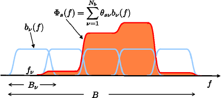
Figure 1: Expansion with overlapping raised cosine pulses.

where the basis $b_{\nu}(f)$ is centered at frequency $f_{\nu},\ \nu=1,\ldots,N_{b}$. The example depicted in Fig. 1 involves (generally overlapping) raised cosine bases with support $B_{\nu}=[f_{\nu}-(1+\rho)/2T_{s},f_{\nu}+(1+\rho)/2T_{s}]$, where $T_{s}$ is the symbol period, and $\rho$ stands for the roll-off factor. Such bases can model transmit-spectra of e.g., multicarrier systems. In other situations, power spectral masks may dictate sharp transitions between contiguous sub-bands, cases in which non-overlapping rectangular bases may be more appropriate. All in all, the set of bases should be selected to accommodate a priori knowledge about the PSD.

The power transmitted by source $s$ will propagate to the location $\mathbf{x}\in\mathbb{R}^{2}$ according to a generally unknown spatial loss function $l_{s}(\mathbf{x}):\mathbb{R}^{2}\to\mathbb{R}$. The propagation model $l_{s}(\mathbf{x})$ not only captures frequency-flat deterministic pathloss, but also stationary, block-fading and even frequency-selective Rayleigh channel effects, since their statistical moments do not depend on the frequency variable. In this case, the following vanishing memory assumption is required on the transmitted signals for the spatial receive-PSD $\Phi(\mathbf{x},f)$ to be factorizable as $l_{s}(\mathbf{x})\Phi_{s}(f)$; see [4] for further details.

(as) Sources $\{u_{s}(t)\}_{s=1}^{N_{s}}$ are stationary, mutually uncorrelated, independent of the channels, and have vanishing correlation per coherence interval; i.e., $r_{ss}(\tau):=E[u_{s}(t+\tau)u_{s}(t)]=0,$ $\forall\>|\tau|>T_{c}-L$, where $T_{c}$ and $L$ represent the coherence interval and delay spread of the channels, respectively.

Under (as), the contribution of source $s$ to the PSD at point $\mathbf{x}$ is $l_{s}(\mathbf{x})\sum_{\nu=1}^{N_{b}}\theta_{s\nu}b_{\nu}(f)$; and the PSD due to all sources received at $\mathbf{x}$ will be given by $\Phi(\mathbf{x},f)=\sum_{s=1}^{N_{s}}l_{s}(\mathbf{x})\sum_{\nu=1}^{N_{b}}\theta_{s\nu}b_{\nu}(f)$. Such a model can be simplified by defining the function $g_{\nu}(\mathbf{x}):=\sum_{s=1}^{N_{s}}\theta_{s\nu}l_{s}(\mathbf{x})$. With this definition and upon exchanging the order of summation, the spatial PSD model takes the form in (1), where functions $\{g_{\nu}(\mathbf{x})\}_{\nu=1}^{N_{b}}$ are to be estimated. They represent the aggregate distribution of power across space corresponding to the frequencies spanned by the bases $\{b_{\nu}\}$. Observe that the sources are not explicitly present in (1). Even if this model could have been postulated directly for the cartography task at hand, the previous discussion justifies the factorization of the $\Phi(\mathbf{x},f)$ map per band in factors depending on each of the variables $\mathbf{x}$ and $f$.

III Cooperative Spline-Based PSD Field Estimation

The sensing strategy will rely on the periodogram estimate $\widehat{\phi}_{rn}(\tau)$ at a set of receiving (sampling) locations $\mathcal{X}:=\{\mathbf{x}_{r}\}_{r=1}^{N_{r}}\in\mathbb{R}^{2}$, frequencies $\mathcal{F}:=\{f_{n}\}_{n=1}^{N}\in B$, and time-slots $\{\tau\}_{\tau=1}^{T}$. In order to reduce the periodogram variance and mitigate fading effects, $\widehat{\phi}_{rn}(\tau)$ is averaged across a window of $T$ time-slots [4], to obtain

$$\varphi_{rn}:=\frac{1}{T}\sum_{\tau=1}^{T}\widehat{\phi}_{rn}(\tau).$$ (3)

Hence, the envisioned setup consists of $N_{r}$ receiving CRs, which collaborate to construct the PSD map based on PSD observations $\{\varphi_{rn}\}$. The bulk of processing is performed centrally at a fusion center (FC), which is assumed to know the position vectors $\mathcal{X}$ of all CRs, and the sensed tones in $\mathcal{F}$. The FC receives over a dedicated control channel, the vector of samples $\bm{\varphi}_{r}:=[\varphi_{r1},\ldots,\varphi_{rN}]^{\prime}\in\mathbb{R}^{N}$ taken by node $r$ for all $r=1,\ldots,N_{r}$.

While a BEM could be introduced for the spatial loss function $l_{s}(\mathbf{x})$ as well [4], the uncertainty on the source locations and obstructions in the propagation medium may render such a model imprecise. This will happen, e.g., when shadowing is present. The alternative approach followed here relies on estimating the functions $g_{\nu}(\mathbf{x})$ based on the data $\{\varphi_{rn}\}$. To capture the smooth portions of $\Phi(\mathbf{x},f)$, the criterion for selecting $g_{\nu}(\mathbf{x})$ will be regularized using a so termed thin-plate penalty [26, p. 30]. This penalty extends to $\mathbb{R}^{2}$ the one-dimensional roughness regularization used in smoothing spline models. Accordingly, functions $\{g_{\nu}\}_{\nu=1}^{N_{b}}$ are estimated as

$$\{\hat{g}_{\nu}\}_{\nu=1}^{N_{b}}:=\arg\min_{\{g_{\nu}\in\mathcal{S}\}}\frac{1}{{N_{r}N}}\sum_{r=1}^{N_{r}}\sum_{n=1}^{N}\left(\varphi_{rn}-\sum_{\nu=1}^{N_{b}}g_{\nu}(\mathbf{x}_{r})b_{\nu}(f_{n})\right)^{2}+\lambda\sum_{\nu=1}^{N_{b}}\int_{\mathbb{R}^{2}}||\nabla^{2}g_{\nu}(\mathbf{x})||_{F}^{2}d\mathbf{x}$$ (4)

where $||\nabla^{2}g_{\nu}||_{F}$ denotes the Frobenius norm of the Hessian of $g_{\nu}$.

The optimization is over $\mathcal{S}$, the space of Sobolev functions, for which the penalty is well defined [10, p. 85]. The parameter $\lambda\geq 0$ controls the degree of smoothing. Specifically, for $\lambda=0$ the estimates in (4) correspond to rough functions interpolating the data; while as $\lambda\to\infty$ the estimates yield linear functions (cf. $\nabla^{2}\hat{g}_{\nu}(\mathbf{x})\equiv\mathbf{0}_{2\times 2}$). A smoothing parameter in between these limiting values will be selected using a leave-one-out cross-validation (CV) approach, as discussed later.

III-A Thin-plate splines solution

The optimization problem (4) is variational in nature, and in principle requires searching over the infinite-dimensional functional space $\mathcal{S}$. It turns out that (4) admits closed-form, finite dimensional minimizers $\hat{g}_{\nu}(\mathbf{x})$, as presented in the following proposition which provides a generalization of standard thin-plate splines results; see e.g., [26, p.31], to the multi-dimensional BEM (1).

Proposition 1: The estimates $\{\hat{g}_{\nu}\}_{\nu=1}^{N_{b}}$ in (4) are thin-plate splines expressible in closed form as

$$\hat{g}_{\nu}(\mathbf{x})=\sum_{r=1}^{N_{r}}\beta_{\nu r}K(||\mathbf{x}-\mathbf{x}_{r}||_{2})+\bm{\alpha}_{\nu 1}^{\prime}\mathbf{x}+\alpha_{\nu 0}$$ (5)

where $K(\rho):=\rho^{2}\log(\rho)$, and $\bm{\beta}_{\nu}:=[\beta_{\nu 1},\ldots,\beta_{\nu N_{r}}]^{\prime}$ is constrained to the linear subspace $\mathcal{B}:=\{\bm{\beta}\in\mathbb{R}^{N_{r}}:\sum_{r=1}^{N_{r}}\beta_{r}=0,\sum_{r=1}^{N_{r}}\beta_{r}\mathbf{x}_{r}=\mathbf{0}_{2},\>\mathbf{x}_{r}\in\mathcal{X}\}$ for $\nu=1,\ldots,N_{b}$.

The proof of this proposition is given in Appendix A.

Remark 1 (Overlapping frequency basis). If the basis functions $\{b_{\nu}(f)\}$ have finite supports which do not overlap, then (4) decouples per $g_{\nu}$, and thus the results in [26, 10] can be applied directly. The novelty of Proposition III-A is that the basis functions with spatial spline coefficients in (1) are allowed to be overlapping. The implication of Proposition III-A is finite parametrization of the PSD map [cf. (5)]. This is particularly important for non-FDMA based CR networks. In the forthcoming Section IV, an overcomplete set $\{b_{\nu}\}$ is adopted in (1), and overlapping bases naturally arise therein.

What is left to determine are the parameters $\alpha:=[\alpha_{10},\bm{\alpha}_{11}^{\prime},\ldots,\alpha_{N_{b}0},\bm{\alpha}_{N_{b}1}^{\prime}]^{\prime}\in\mathbb{R}^{3N_{b}}$, and $\bm{\beta}:=[\bm{\beta}_{1}^{\prime},\ldots,\bm{\beta}_{N_{b}}^{\prime}]^{\prime}\in\mathbb{R}^{N_{r}N_{b}}$ in (5). To this end, define the vector $\bm{\varphi}:=[\varphi_{11},\ldots,\varphi_{1N},\ldots,\varphi_{N_{r}1},\ldots,\varphi_{N_{r}N}]^{\prime}\in\mathbb{R}^{{N_{r}N}}$ containing the network-wide data obtained at all frequencies in $\mathcal{F}$. Three matrices are also introduced collecting the regression inputs: i) $\mathbf{T}\in\mathbb{R}^{N_{r}\times 3}$ with $r$th row $\mathbf{t}_{r}^{\prime}:=[1\>\mathbf{x}_{r}^{\prime}]$ for $r=1,\ldots,N_{r}$ and $\mathbf{x}_{r}\in\mathcal{X}$; ii) $\mathbf{B}\in\mathbb{R}^{N\times N_{b}}$ with $n$th row $\mathbf{b}_{n}^{\prime}:=[b_{1}(f_{n}),\ldots,b_{N_{b}}(f_{n})]$ for $n=1,\ldots,N$; and iii) $\mathbf{K}\in\mathbb{R}^{N_{r}\times N_{r}}$ with $ij$-th entry $[\mathbf{K}]_{ij}:=K(||\mathbf{x}_{i}-\mathbf{x}_{j}||)$ for $\mathbf{x}_{i},\mathbf{x}_{j}\in\mathcal{X}$. Consider also the QR decompositions of $\mathbf{T}=\left[\mathbf{Q}_{1}\>\mathbf{Q}_{2}\right]\left[\mathbf{R}^{\prime}\ \mathbf{0}\right]^{\prime}$ and $\mathbf{B}=\left[\bm{\Omega}_{1}\>\bm{\Omega}_{2}\right]\left[\bm{\Gamma}^{\prime}\ \mathbf{0}\right]^{\prime}$.

Upon plugging (5) into (4), it is shown in Appendix B that the optimal $\{\bm{\alpha},\bm{\beta}\}$ satisfy the following system of equations

$$(\mathbf{B}\otimes\mathbf{Q}_{2}^{\prime})\bm{\varphi} =\left[(\mathbf{B}^{\prime}\mathbf{B}\otimes\mathbf{Q}_{2}^{\prime}\mathbf{K}\mathbf{Q}_{2})+{N_{r}N}\lambda\mathbf{I}_{N_{b}(N_{r}-3)}\right]\hat{\bm{\gamma}}$$ (6)

$$[\bm{\Gamma}\otimes\mathbf{R}]\hat{\bm{\alpha}} =(\bm{\Omega}_{1}^{\prime}\otimes\mathbf{Q}_{1}^{\prime})\bm{\varphi}-(\bm{\Gamma}\otimes\mathbf{Q}_{1}^{\prime}\mathbf{K}\mathbf{Q}_{2})\hat{\bm{\gamma}}$$ (7)

$$\hat{\bm{\beta}} =(\mathbf{I}_{N_{b}}\otimes\mathbf{Q}_{2})\hat{\bm{\gamma}}.$$ (8)

Matrix $\mathbf{Q}_{2}^{\prime}\mathbf{K}\mathbf{Q}_{2}$ is positive definite, and $\textrm{rank}(\bm{\Gamma}\otimes\mathbf{R})=\textrm{rank}(\bm{\Gamma})\textrm{rank}(\mathbf{R})$; see e.g., [18]. It thus follows that (6)-(7) admit a unique solution if and only if $\bm{\Gamma}$ and $\mathbf{R}$ are invertible (correspondingly, $\mathbf{B}$ and $\mathbf{T}$ have full column rank). These conditions place practical constraints that should be taken into account at the system design stage. Specifically, $\mathbf{T}$ has full column rank if and only if the points in $\mathcal{X}$, i.e., the CR locations, are not aligned. Furthermore, $\mathbf{B}$ will have linearly independent columns provided the basis functions $\{b_{\nu}(f)\}_{\nu=1}^{N_{b}}$ comprise a linearly independent and complete set, i.e., $B\subseteq\bigcup_{\nu}B_{\nu}$. Note that completeness precludes all frequencies $\{f_{n}\}_{n=1}^{N}$ from falling outside the aggregate support of the basis set, hence preventing undesired all-zero columns in $\mathbf{B}$.

Remark 2 (Practicality of uniqueness conditions). The condition on $\mathcal{X}$ does not introduce an actual limitation as it can be easily satisfied in practice, especially when the CRs are randomly deployed. Likewise, the basis set is part of the system design, and can be chosen to satisfy the conditions on $\mathbf{B}$. Nonetheless, these conditions will be bypassed in Section IV by allowing for an overcomplete set of functions $\{b_{\nu}\}$.

The combined results in this section can be summarized in the following steps constituting the spline-based spectrum cartography algorithm, which amounts to estimating $\Phi(\mathbf{x},f)$:

S1.

Given $\bm{\varphi}$, solve (6)-(8) for $\bm{\hat{\alpha}},\bm{\hat{\beta}}$, after selecting $\lambda$ as detailed in Appendix D.

S2.

Substitute $\bm{\hat{\alpha}}$ and $\bm{\hat{\beta}}$ into (5) to obtain $\{\hat{g}_{\nu}(\mathbf{x})\}_{\nu=1}^{N_{b}}$.

S3.

Use $\{\hat{g}_{\nu}(\mathbf{x})\}_{\nu=1}^{N_{b}}$ in (1) to estimate $\Phi(\mathbf{x},f)$.

III-B PSD tracker

The real-time requirements on the sensing radios and the convenience of an estimator that adapts to changes in the spectrum map are the motivating reasons behind the PSD tracker introduced in this section. The spectrum map estimator will be henceforth denoted by $\Phi(\mathbf{x},f,\tau)$, to make its time dependence explicit.

Define the vector $\bm{\widehat{\phi}}_{n}(\tau):=[\widehat{\phi}_{1n}(\tau),\ldots,\widehat{\phi}_{N_{r}n}(\tau)]^{\prime}$ of periodogram samples taken at frequency $f_{n}$ by all CRs, and form the supervector $\bm{\widehat{\phi}}(\tau):=[\bm{\widehat{\phi}}_{1}^{\prime}(\tau),\ldots,\bm{\widehat{\phi}}_{N}^{\prime}(\tau)]^{\prime}\in\mathbb{R}^{N_{r}N}$. Per time-slot $\tau=1,2,\ldots$, the periodogram $\widehat{\bm{\phi}}(\tau)$ is averaged using the following adaptive counterpart of (3):

$$\bm{\varphi}(\tau):=\sum_{\tau^{\prime}=1}^{\tau}\delta^{\tau-\tau^{\prime}}\widehat{\bm{\phi}}(\tau^{\prime})=\delta\bm{\varphi}(\tau-1)+\widehat{\bm{\phi}}(\tau)$$ (9)

which implements an exponentially weighted moving average operation with forgetting factor $\delta\in(0,1)$. For every $\tau$, the online estimator $\Phi(\mathbf{x},f,\tau)$ is obtained by plugging in (1) the solution $\{\hat{g}_{\nu}(\mathbf{x},\tau)\}_{\nu=1}^{N_{b}}$ of (4), after replacing $\varphi_{rn}$ with $\varphi_{rn}(\tau)$ [cf. the entries of the vector in (9)]. In addition to mitigating fading effects, this adaptive approach can track slowly time-varying PSDs because the averaging in (9) exponentially discards past data.

Suppose that per time-slot $\tau$, the FC receives raw periodogram samples $\bm{\widehat{\phi}}(\tau)$ from the CRs in order to update $\Phi(\mathbf{x},f,\tau)$. The results of Section III apply for every $\tau$, meaning that $\{\hat{g}_{\nu}(\mathbf{x},\tau)\}_{\nu=1}^{N_{b}}$ are given by (5), while the optimum coefficients $\{\hat{\bm{\alpha}}(\tau),\hat{\bm{\beta}}(\tau)\}$ are found after solving (6)-(8). Capitalizing on (9), straightforward manipulations of (6)-(8) show that $\{\hat{\bm{\alpha}}(\tau),\hat{\bm{\beta}}(\tau)\}$ are recursively given for all $\tau\geq 1$ by

$$\hat{\bm{\beta}}(\tau) =\delta\hat{\bm{\beta}}(\tau-1)+(\mathbf{I}_{N_{b}}\otimes\mathbf{Q}_{2})\mathbf{G}_{1}\widehat{\bm{\phi}}(\tau)$$ (10)

$$\hat{\bm{\alpha}}(\tau) =\delta\hat{\bm{\alpha}}(\tau-1)+\mathbf{G}_{2}\widehat{\bm{\phi}}(\tau)$$ (11)

where the time-invariant matrices $\mathbf{G}_{1}$ and $\mathbf{G}_{2}$ are

$$\mathbf{G}_{1} :=\left[(\mathbf{B}^{\prime}\mathbf{B}\otimes\mathbf{Q}_{2}^{\prime}\mathbf{K}\mathbf{Q}_{2})+{N_{r}N}\lambda\mathbf{I}_{N_{b}(N_{r}-3)}\right]^{-1}(\mathbf{B}\otimes\mathbf{Q}_{2}^{\prime})$$

$$\mathbf{G}_{2} :=[\bm{\Gamma}\otimes\mathbf{R}]^{-1}\left[(\bm{\Omega}_{1}^{\prime}\otimes\mathbf{Q}_{1}^{\prime})-(\bm{\Gamma}\otimes\mathbf{Q}_{1}^{\prime}\mathbf{K}\mathbf{Q}_{2})\mathbf{G}_{1}\right].$$

Recursions (10)-(11) provide a means to update $\Phi(\mathbf{x},f,\tau)$ sequentially in time, by incorporating the newly acquired data from the CRs in $\widehat{\bm{\phi}}(\tau)$. There is no need to separately update $\bm{\varphi}(\tau)$ as in (9), yet the desired averaging takes place. Furthermore, matrices $\mathbf{G}_{1}$ and $\mathbf{G}_{2}$ need to be computed only once, during the startup phase of the network.

IV Group-Lasso on Splines

An improved spline-based PSD estimator is developed in this section to fit the unknown spatial functions $\{g_{\nu}\}_{\nu=1}^{N_{b}}$ in the model $\Phi(\mathbf{x},f)=\sum_{\nu=1}^{N_{b}}g_{\nu}(\mathbf{x})b_{\nu}(f)$, with a large ($N_{b}\gg N_{r}N$), and a possibly overcomplete set of known basis functions $\{b_{\nu}\}_{\nu=1}^{N_{b}}$. These models are particularly attractive when there is an inherent uncertainty on the transmitters’ parameters, such as central frequency and bandwidth of the pulse shapers; or, e.g., the roll-off factor when raised-cosine pulses are employed. In particular, adaptive communication schemes rely on frequently adjusting these parameters [12, Ch. 9]. A sizeable collection of bases to effectively accommodate most of the possible cases provides the desirable robustness. Still, prior knowledge available on the incumbent communication technologies being sensed should be exploited to choose the most descriptive classes of basis functions; e.g., a large set of raised-cosine pulses. This knowledge justifies why known bases are selected to describe frequency characteristics of the PSD map, while a variational approach is preferred to capture spatial dependencies.

In this context, the envisioned estimation method should provide the CRs with the capability of selecting a few bases that “better explain” the actual transmitted signals. As a result, most functions $g_{\nu}$ are expected to be identically zero; hence, there is an inherent form of sparsity present that can be exploited to improve estimation. The rationale behind the proposed approach can be rooted in the basis pursuit principle, a term coined in [8] for finding the most parsimonious sparse signal expansion using an overcomplete basis set. A major differentiating aspect however, is that while the sparse coefficients in the basis expansions treated in [8] are scalars, model (1) here entails bases weighted by functions $g_{\nu}$.

The proposed approach to sparsity-aware spline-based field estimation from the space-frequency power spectrum measurements $\varphi_{rn}$ [cf. (3)], is to obtain $\{\hat{g}_{\nu}\}_{\nu=1}^{N_{b}}$ as

$$\{\hat{g}_{\nu}\}_{\nu=1}^{N_{b}}:=\arg\min_{\{g_{\nu}\in\mathcal{S}\}} \frac{1}{{N_{r}N}}\sum_{r=1}^{N_{r}}\sum_{n=1}^{N}\left(\varphi_{rn}-\sum_{\nu=1}^{N_{b}}g_{\nu}(\mathbf{x}_{r})b_{\nu}(f_{n})\right)^{2}+\lambda\sum_{\nu=1}^{N_{b}}\int_{\mathbb{R}^{2}}||\nabla^{2}g_{\nu}(\mathbf{x})||_{F}^{2}d\mathbf{x}$$ (12)

$$+\mu\sum_{\nu=1}^{N_{b}}\left\|\left[g_{\nu}(\mathbf{x}_{1}),\ldots,g_{\nu}(\mathbf{x}_{N_{r}})\right]^{\prime}\right\|_{2}.$$

Relative to (4), the cost here is augmented with an additional regularization term weighted by a tuning parameter $\mu\geq 0$. Clearly, if $\mu=0$ then (12) boils down to (4). To appreciate the role of the new penalty term, note that the minimization of $\left\|\left[g_{\nu}(\mathbf{x}_{1}),\ldots,g_{\nu}(\mathbf{x}_{N_{r}})\right]^{\prime}\right\|_{2}$ intuitively shrinks all pointwise functional values $\left\{g_{\nu}(\mathbf{x}_{1}),\ldots,g_{\nu}(\mathbf{x}_{N_{r}})\right\}$ to zero for sufficiently large $\mu$. Interestingly, it will be shown in the ensuing section that this is enough to guarantee that $\hat{g}_{\nu}(\mathbf{x})\equiv 0\ \forall\mathbf{x}$, for $\mu$ large enough.

IV-A Estimation using the group-Lasso

Consider the classical problem of linear regression; see, e.g. [13, p. 11], where a vector $\mathbf{y}\in\mathbb{R}^{n}$ of observations is available, along with a matrix $\mathbf{X}\in\mathbb{R}^{n\times p}$ of inputs. The group Lasso estimate for the vector of features $\bm{\zeta}:=[\bm{\zeta}_{1}^{\prime},\ldots,\bm{\zeta}_{N_{b}}^{\prime}]^{\prime}\in\mathbb{R}^{p}$ is defined as the solution to [3, 29]

$$\min_{\bm{\zeta}}\frac{1}{2}\left\|\mathbf{y}-\mathbf{X}\bm{\zeta}\right\|_{2}^{2}+\mu\sum_{\nu=1}^{N_{b}}\|\bm{\zeta}_{\nu}\|_{2}.$$ (13)

This criterion achieves model selection by retaining relevant factors $\bm{\zeta}_{\nu}\in\mathbb{R}^{p/N_{b}}$ in which the features are grouped. In other words, group-Lasso encourages sparsity at the factor level, either by shrinking to zero all variables within a factor, or by retaining them altogether depending on the value of the tuning parameter $\mu\geq 0$. As $\mu$ is increased, more sub-vector estimates $\bm{\zeta}_{\nu}$ become zero, and the corresponding factors drop out of the model. It can be shown from the Karush-Kuhn-Tucker optimality conditions that only for $\mu\geq\mu_{\max}:=\max_{i}\|\mathbf{X}_{i}^{\prime}\mathbf{y}\|_{2}$ it holds that $\bm{\zeta}_{1}=\ldots=\bm{\zeta}_{N_{b}}=\mathbf{0}_{p/N_{b}}$, so that the values of interest are $\mu\in[0,\mu_{\max}]$ [2].

The connection between (13) and the spline-based field estimator (12) builds on Proposition III-A, which still holds in this context. That is, even though criteria (4) and (12) purposely differ, their respective solutions $\hat{g}_{\nu}(\mathbf{x})$ have the same form in (5). Indeed, the adaptation of the proof in Appendix A to the new case is straightforward, since the additional penalty term in (12) depends on $g_{\nu}$ evaluated at the knots. The essential difference manifested by this penalty is revealed when estimating the parameters $\bm{\alpha}$ and $\bm{\beta}$ in (5), as presented in the following proposition.

Proposition 2: The spline-based field estimator (12) is equivalent to group-Lasso (13), under the identities

$$\mathbf{y} :=\frac{1}{\sqrt{N_{r}N}}[\bm{\varphi}^{\prime},\>\bm{0}]^{\prime},\quad\mathbf{X}:=\frac{1}{\sqrt{N_{r}N}}\left[\begin{array}[]{c}\mathbf{B}\otimes\mathbf{I}_{N_{r}}\\ \mathbf{I}_{N_{b}}\otimes\left\{\textrm{bdiag}(({N_{r}N}\lambda\mathbf{Q}_{2}^{\prime}\mathbf{K}\mathbf{Q}_{2})^{1/2},\mathbf{0})[\mathbf{KQ}_{2}\>\>\mathbf{T}]^{-1}\right\}\end{array}\right]$$ (16)

with their respective solutions related by

$$\hat{g}_{\nu}(\mathbf{x}) =\sum_{r=1}^{N_{r}}\beta_{\nu r}K(||\mathbf{x}-\mathbf{x}_{r}||_{2})+\bm{\alpha}_{\nu 1}^{\prime}\mathbf{x}+\alpha_{\nu 0}$$ (17)

$$\left[\bm{\beta}_{\nu}^{\prime},\bm{\alpha}_{\nu}^{\prime}\right]^{\prime} =\textrm{bdiag}(\mathbf{Q}_{2},\mathbf{I}_{3})[\mathbf{KQ}_{2}\>\>\mathbf{T}]^{-1}\hat{\bm{\zeta}}_{\nu}$$ (18)

where $\bm{\beta}_{\nu}:=[\beta_{\nu 1},\ldots,\beta_{\nu N_{r}}]^{\prime}$ and $\bm{\alpha}_{\nu}:=[\alpha_{\nu 0},\bm{\alpha}_{\nu 1}^{\prime}]^{\prime}$.

The factors $\{\bm{\zeta}_{\nu}\}_{\nu=1}^{N_{b}}$ in (13) are in one-to-one correspondence with the vectors $\{[{\bm{\beta}}_{\nu}^{\prime},{\bm{\alpha}}_{\nu}^{\prime}]^{\prime}\}_{\nu=1}^{N_{b}}$ through the linear mapping (18). This implies that whenever a factor $\bm{\zeta}_{\nu}$ is dropped from the linear regression model obtained after solving (13), then $\hat{g}_{\nu}(\mathbf{x})\equiv 0$, and the term corresponding to $b_{\nu}(f)$ does not contribute to (1). Hence, by appropriately selecting the value of $\mu$, criterion (12) has the potential of retaining only the most significant terms in $\Phi(\mathbf{x},f)=\sum_{\nu=1}^{N_{b}}g_{\nu}(\mathbf{x})b_{\nu}(f)$, and thus yields parsimonious PSD map estimates. All in all, the motivation behind the variational problem (12) is now unravelled. The additional penalty term not present in (4) renders (12) equivalent to a group-Lasso problem. This enforces sparsity in the parameters of the splines expansion for $\Phi(\mathbf{x},f)$ at a factor level, which is exactly what is needed to potentially null the less descriptive functions $g_{\nu}$.

Remark 3 (Comparison with the PSD map estimator in Section III). The sparsity-agnostic LS problem (4) will not give rise to identically zero vectors $\{\bm{\alpha}_{\nu},\bm{\beta}_{\nu}\}$, for any $\nu$. Even when $N_{b}$ is not large, a sparsity-aware estimator will perform better if the underlying PSD is generated by a few basis functions. This is expected since the out-of-band residual error will increase when all basis functions enter the model (1); see also [4] for a related assessment. What is more, when the number of bases is sufficiently large ($N_{b}\gg{N_{r}N}$) matrix $\mathbf{B}$ is fat, and the approach in Section III is not applicable . On the other hand, it is admittedly more complex computationally to solve (13) than the system of linear equations (6)-(8). Because (12) is not a linear smoother, a leave-one-out (bi-) CV approach to select the tuning parameters $\lambda$ and $\mu$ does not enjoy the computational savings detailed in Appendix D. $K$-fold CV can be utilized instead, with typical choices of $K=5$ or $10$, as suggested in [13, p. 242].

The group-Lassoed splines-based approach to spectrum cartography developed in this section can be summarized in the following steps to estimate the global PSD map $\Phi(\mathbf{x},f)$:

S1.

Given $\bm{\varphi}$ and utilizing any group Lasso solver, obtain $\hat{\bm{\zeta}}:=[\hat{\bm{\zeta}}_{1}^{\prime},\ldots,\hat{\bm{\zeta}}_{N_{b}}^{\prime}]^{\prime}$ by solving (13).

S2.

Form the estimates $\bm{\hat{\alpha}},\bm{\hat{\beta}}$ using the change of variables $[\hat{\bm{\beta}}_{\nu}^{\prime},\hat{\bm{\alpha}}_{\nu}^{\prime}]^{\prime}=\textrm{bdiag}(\mathbf{Q}_{2},\mathbf{I}_{3})[\mathbf{KQ}_{2}\>\>\mathbf{T}]^{-1}\hat{\bm{\zeta}}_{\nu}$ for $\nu=1,\ldots,N_{b}$.

S3.

Substitute $\bm{\hat{\alpha}}$ and $\bm{\hat{\beta}}$ into (17) to obtain $\{\hat{g}_{\nu}(\mathbf{x})\}_{\nu=1}^{N_{b}}$.

S4.

Use $\{\hat{g}_{\nu}(\mathbf{x})\}_{\nu=1}^{N_{b}}$ in (1) to estimate $\Phi(\mathbf{x},f)$.

Implementing S1-S4 presumes that CRs communicate their local PSD estimates to a fusion center, which uses their aggregation in $\bm{\varphi}$ to estimate the field. But what if an FC is not available for centrally running S1-S4? In certain cases, forgoing with an FC is reasonable when the designer wishes to avoid an isolated point of failure, or, aims at a network topology which scales well with an increasing number of CRs based on power considerations (CRs located far away from the FC will drain their batteries more to reach the FC). These reasons motivate well a fully distributed counterpart of S1-S4, which is pursued next.

V Distributed Group-Lasso for In-Network Spectrum Cartography

Consider $N_{r}$ networked CRs that are capable of sensing the ambient RF spectrum, performing some local computations, as well as exchanging messages among neighbors via dedicated control channels. In lieu of a fusion center, the CR network is naturally modeled as an undirected graph ${\cal G}({\cal R},{\cal E})$, where the vertex set ${\cal R}:=\{1,\ldots,N_{r}\}$ corresponds to the sensing radios, and the edges in ${\cal E}$ represent pairs of CRs that can communicate. Radio $r\in{\cal R}$ communicates with its single-hop neighbors in ${\cal N}_{r}$, and the size of the neighborhood is denoted by $|{\cal N}_{r}|$. The locations $\{\mathbf{x}_{r}\}_{r=1}^{N_{r}}:=\mathcal{X}$ of the sensing radios are assumed known to the CR network. To ensure that the measured data from an arbitrary CR can eventually percolate throughout the entire network, it is assumed that the graph ${\cal G}$ is connected; i.e., there exists a (possibly) multi-hop communication path connecting any two CRs.

For the purpose of estimating an unknown vector $\bm{\zeta}:=\left[\bm{\zeta}_{1}^{\prime},\ldots,\bm{\zeta}_{N_{b}}^{\prime}\right]^{\prime}\in\mathbb{R}^{p}$, each radio $r\in{\cal R}$ has available a local vector of observations $\mathbf{y}_{r}\in\mathbb{R}^{n_{r}}$ as well as its own matrix of inputs $\mathbf{X}_{r}\in\mathbb{R}^{n_{r}\times p}$. Radios collaborate to form the wanted group-Lasso estimator (13) in a distributed fashion, using

$$\hat{\bm{\zeta}}_{\textrm{glasso}}=\mbox{arg}\>\min_{\bm{\zeta}}\frac{1}{2}\sum_{r=1}^{N_{r}}\left\|\mathbf{y}_{r}-\mathbf{X}_{r}\bm{\zeta}\right\|_{2}^{2}+\mu\sum_{\nu=1}^{N_{b}}\|\bm{\zeta}_{\nu}\|_{2}$$ (19)

where ${\mathbf{y}}:=[{\mathbf{y}}_{1}^{\prime},\ldots,{\mathbf{y}}_{N_{r}}^{\prime}]^{\prime}\in\mathbb{R}^{n\times 1}$ with $n:=\sum_{r=1}^{N_{r}}n_{r}$, and ${\mathbf{X}}:=[{\mathbf{X}}_{1}^{\prime},\ldots,{\mathbf{X}}_{N_{r}}^{\prime}]^{\prime}\in\mathbb{R}^{n\times p}$. The motivation behind developing a distributed solver of (19) is to tackle (12) based on in-network processing of the local observations $\bm{\varphi}_{r}:=[\varphi_{r1},\ldots,\varphi_{rN}]^{\prime}$ available per radio [cf. (3)]. Indeed, it readily follows that (19) can be used instead of (13) in Proposition IV-A when

$$\mathbf{y}_{r}:=\frac{1}{\sqrt{N_{r}N}}\left[\begin{array}[]{c}\bm{\varphi}_{r}\\ \mathbf{0}\end{array}\right],\quad\mathbf{X_{r}}:=\frac{1}{\sqrt{N_{r}N}}\left[\begin{array}[]{c}\mathbf{B}\otimes\mathbf{e}_{N_{r},r}^{\prime}\\ \mathbf{I}_{N_{b}}\otimes\left[\textrm{bdiag}((N_{r}N\lambda\mathbf{Q}_{2}^{\prime}\mathbf{K}\mathbf{Q}_{2})^{1/2},\mathbf{0})[\mathbf{KQ}_{2}\>\>\mathbf{T}]^{-1}\right]\end{array}\right],\quad r\in{\cal R}$$

corresponding to the identifications $n_{r}=N$ $\forall r\in{\cal R}$, $p=N_{b}N_{r}$. Note that because the locations $\{\mathbf{x}_{r}\}$ are assumed known to the entire network, CR $r$ can form matrices $\mathbf{T}$, $\mathbf{K}$, and thus, the local regression matrix $\mathbf{X}_{r}$.

V-A Consensus-based reformulation of the group-Lasso

To distribute the cost in (19), replace the global variable $\bm{\zeta}$ which couples the per-agent summands with local variables $\{\bm{\zeta}_{r}\}_{r=1}^{N_{r}}$ representing candidate estimates of $\bm{\zeta}$ per sensing radio. It is now possible to reformulate (19) as a convex constrained minimization problem

$$\left\{\hat{\bm{\zeta}}_{r}\right\}_{r=1}^{N_{r}}= \>\mbox{arg}\>\min_{\{\bm{\zeta}_{r}\}}\frac{1}{2}\sum_{r=1}^{N_{r}}\left[\left\|\mathbf{y}_{r}-\mathbf{X}_{r}\bm{\zeta}_{r}\right\|_{2}^{2}+\frac{2\mu}{N_{r}}\sum_{\nu=1}^{N_{b}}\|\bm{\zeta}_{r\nu}\|_{2}\right]$$ (20)

$$\begin{array}[]{ccl}\mbox{ s. t.}&}{}{\hfil&\bm{\zeta}_{r}=\bm{\zeta}_{r^{\prime}},{\>}r\in{\cal R},{\>}r^{\prime}\in{\cal N}_{r},\ \bm{\zeta}_{r}:=\left[\bm{\zeta}_{r1}^{\prime},\ldots,\bm{\zeta}_{rN_{b}}^{\prime}\right]^{\prime}.\end{array}$$ (22)

The equality constraints directly effect local agreement across each CR’s neighborhood. Since the communication graph $\mathcal{G}$ is assumed connected, these constraints also ensure global consensus a fortiori, meaning that $\bm{\zeta}_{r}=\bm{\zeta}_{r^{\prime}},$ $\forall r,r^{\prime}\in{\cal R}$. Indeed, let $P(r,r^{\prime}):r,r_{1},r_{2},\ldots,r_{n},r^{\prime}$ denote a path on $\mathcal{G}$ that joins an arbitrary pair of CRs $(r,r^{\prime})$. Because contiguous radios in the path are neighbors by definition, the corresponding chain of equalities $\bm{\zeta}_{r}=\bm{\zeta}_{r_{1}}=\bm{\zeta}_{r_{2}}=\ldots=\bm{\zeta}_{r_{n}}=\bm{\zeta}_{r^{\prime}}$ dictated by the constraints in (20) imply $\bm{\zeta}_{r}=\bm{\zeta}_{r^{\prime}}$, as desired. Thus, the constraints can be eliminated by replacing all the $\{\bm{\zeta}_{r}\}$ with a common $\bm{\zeta}$, in which case the cost in (20) reduces to the one in (19). This argument establishes the following result.

Lemma 1: If $\mathcal{G}$ is a connected graph, (19) and (20) are equivalent optimization problems, in the sense that $\hat{\bm{\zeta}}_{\textrm{glasso}}=\hat{\bm{\zeta}}_{r},{\>}\forall{\>}r\in\mathcal{R}.$

Problem (20) will be modified further for the purpose of reducing the computational complexity of the resulting algorithm. To this end, for a given $\mathbf{a}\in\mathbb{R}^{p}$ consider the problem

$$\min_{\bm{\zeta}} \frac{1}{2}||\bm{\zeta}||_{2}^{2}-\mathbf{a}^{\prime}\bm{\zeta}+\mu\sum_{\nu=1}^{N_{b}}\|\bm{\zeta}_{\nu}\|_{2},\hskip 28.45274pt\bm{\zeta}:=[\bm{\zeta}_{1}^{\prime},\ldots,\bm{\zeta}_{N_{b}}^{\prime}]^{\prime}$$ (23)

and notice that it is separable in the $N_{b}$ subproblems

$$\min_{\bm{\zeta}_{\nu}} \frac{1}{2}||\bm{\zeta}_{\nu}||_{2}^{2}-\mathbf{a}_{\nu}^{\prime}\bm{\zeta}_{\nu}+\mu\|\bm{\zeta}_{\nu}\|_{2},\hskip 28.45274pt\mathbf{a}:=[\mathbf{a}_{1}^{\prime},\ldots,\mathbf{a}_{N_{b}}^{\prime}]^{\prime}.$$ (24)

Interestingly, each of these subproblems admits a closed-form solution as given in the following lemma.

Lemma 2: The minimizer $\bm{\zeta}^{\star}_{\nu}$ of (24) is obtained via the vector soft-thresholding operator $\mathcal{T}_{\mu}(\cdot)$ defined by

$$\bm{\zeta}_{\nu}^{\star}=\mathcal{T}_{\mu}(\mathbf{a}_{\nu}):=\frac{\mathbf{a}_{\nu}}{\|\mathbf{a}_{\nu}\|_{2}}\left(\|\mathbf{a}_{\nu}\|_{2}-\mu\right)_{+}$$ (25)

where $\left(\cdot\right)_{+}:=\max\{\cdot,0\}$ .

Problem (23) is an instance of the group-Lasso (13) when $\mathbf{X}^{\prime}\mathbf{X}=\mathbf{I}_{p}$, and $\mathbf{a}:=\mathbf{X}^{\prime}{\mathbf{y}}$. As such, result (25) can be viewed as a particular case of the operators in [22] and [28]. However it is worth to prove Lemma V-A directly, since in this case the special form of (24) renders the proof neat in its simplicity.

Proof: It will be argued that the solver of (24) takes the form $\bm{\zeta}_{\nu}^{\star}=t\mathbf{a}_{\nu}$ for some scalar $t\geq 0$. This is because among all $\bm{\zeta}_{\nu}$ with the same $\ell_{2}$-norm, the Cauchy-Schwarz inequality implies that the maximizer of $\mathbf{a}_{\nu}^{\prime}\bm{\zeta}_{\nu}$ is colinear with (and in the same direction of) $\mathbf{a}_{\nu}$. Substituting $\bm{\zeta}_{\nu}=t\mathbf{a}_{\nu}$ into (24) renders the problem scalar in $t\geq 0$, with solution $t^{\star}=\left(\|\mathbf{a}_{\nu}\|-\mu\right)_{+}/\left({2\|\mathbf{a}_{\nu}\|}\right)$, which completes the proof.

In order to take advantage of Lemma V-A, auxiliary variables $\bm{\gamma}_{r},\ r=1,\ldots,N_{r}$ are introduced as copies of $\bm{\zeta}_{r}$. Upon introducing appropriate constraints $\bm{\gamma}_{r}=\bm{\zeta}_{r}$ that guarantee the equivalence of the formulations along the lines of Lemma V-A, problem (20) can be recast as

$$\left\{\hat{\bm{\zeta}}_{r}\right\}_{r=1}^{N_{r}}= \hskip 8.5359pt\mbox{arg}\min_{\{\bm{\zeta}_{r},\bm{\gamma}_{r},\bm{\gamma}_{r}^{r^{\prime}}\}}\frac{1}{2}\sum_{r=1}^{N_{r}}\left[\left\|\mathbf{y}_{r}-\mathbf{X}_{r}\bm{\gamma}_{r}\right\|_{2}^{2}+\frac{2\mu}{N_{r}}\sum_{\nu=1}^{N_{b}}\|\bm{\zeta}_{r\nu}\|_{2}\right]$$ (26)

$$\begin{array}[]{ccl}\mbox{ s. to}&}{}{\hfil&\bm{\zeta}_{r}=\bm{\gamma}_{r}^{r^{\prime}}=\bm{\zeta}_{r^{\prime}},{\>}r\in{\cal R},{\>}r^{\prime}\in{\cal N}_{r}\\ &&\bm{\gamma}_{r}=\bm{\zeta}_{r},\ r\in{\cal R}.\end{array}$$ (29)

The dummy variables $\bm{\gamma}_{r}^{r^{\prime}}$ are inserted for technical reasons that will become apparent in the ensuing section, and will be eventually eliminated.

V-B Distributed group-Lasso algorithm

The distributed group-Lasso algorithm is constructed by optimizing (26) using the alternating direction method of multipliers (AD-MoM) [6]. In this direction, associate Lagrange multipliers ${\mathbf{v}}_{r},\bar{{\mathbf{v}}}_{r}^{r^{\prime}}$ and $\breve{{\mathbf{v}}}_{r}^{r^{\prime}}$ with the constraints $\bm{\gamma}_{r}=\bm{\zeta}_{r}$, $\bm{\zeta}_{r^{\prime}}=\bm{\gamma}_{r}^{r^{\prime}}$ and $\bm{\zeta}_{r}=\bm{\gamma}_{r}^{r^{\prime}}$, respectively, and consider the augmented Lagrangian with parameter $c>0$

$${\mathcal{L}}_{c}\left[\{\bm{\zeta}_{r}\},\bm{\gamma},\bm{{\mathit{v}}}\right]= \frac{1}{2}\sum_{r=1}^{N_{r}}\left[\left\|\mathbf{y}_{r}-\mathbf{X}_{r}\bm{\gamma}_{r}\right\|_{2}^{2}+\frac{2\mu}{N_{r}}\sum_{\nu=1}^{N_{b}}\|\bm{\zeta}_{r\nu}\|_{2}\right]+\sum_{r=1}^{N_{r}}{\mathbf{v}}_{r}^{\prime}(\bm{\zeta}_{r}-\bm{\gamma}_{r})+\frac{c}{2}\sum_{r=1}^{N_{r}}\|\bm{\zeta}_{r}-\bm{\gamma}_{r}\|_{2}^{2}$$

$$+\sum_{r=1}^{N_{r}}\sum_{r^{\prime}\in{\cal N}_{r}}\left[(\breve{{\mathbf{v}}}_{r}^{r^{\prime}})^{\prime}(\bm{\zeta}_{r}-{\bm{\gamma}}_{r}^{r^{\prime}})+(\bar{{\mathbf{v}}}_{r}^{r^{\prime}})^{\prime}(\bm{\zeta}_{r^{\prime}}-{\bm{\gamma}}_{r}^{r^{\prime}})\right]+\frac{c}{2}\sum_{r=1}^{N_{r}}\sum_{r^{\prime}\in{\cal N}_{r}}\left[\|\bm{\zeta}_{r}-{\bm{\gamma}}_{r}^{r^{\prime}}\|_{2}^{2}+\|\bm{\zeta}_{r^{\prime}}-{\bm{\gamma}}_{r}^{r^{\prime}}\|_{2}^{2}\right]$$ (30)

where for notational convenience we group the variables $\bm{\gamma}:=\{\bm{\gamma}_{r},\{{\bm{\gamma}}_{r}^{r^{\prime}}\}_{r^{\prime}\in{\cal N}_{r}}\}_{r\in{\cal R}}$, and multipliers
$\bm{{\mathit{v}}}:=\{{\mathbf{v}}_{r},\{\breve{{\mathbf{v}}}_{r}^{r^{\prime}}\}_{r^{\prime}\in{\cal N}_{r}},\{\bar{{\mathbf{v}}}_{r}^{r^{\prime}}\}_{r^{\prime}\in{\cal N}_{r}}\}_{r\in{\cal R}}$.

Application of the AD-MoM to the problem at hand consists of a cycle of ${\mathcal{L}}_{c}$ minimizations in a block-coordinate fashion w.r.t. $\{\bm{\zeta}_{r}\}$ firstly, and $\bm{\gamma}$ secondly, together with an update of the multipliers per iteration $k=0,1,2,\ldots$. Deferring the details to Appendix E, the four main properties of this procedure that are instrumental to the resulting algorithm can be highlighted as follows.

1. Thanks to the introduction of the local copies $\bm{\zeta}_{r}$ and the dummy variables $\bm{\gamma}_{r}^{r^{\prime}}$, the minimizations of ${\mathcal{L}}_{c}$ w.r.t. both $\{\bm{\zeta}_{r}\}$ and $\bm{\gamma}$ decouple per CR $r$, thus enabling distribution of the algorithm. Moreover, the constraints in (26) involve variables of neighboring CRs only, which allows the required communications to be local within each CR’s neighborhood.

2. Introduction of the variables $\bm{\gamma}_{r}$ separates the quadratic cost $\|{\mathbf{y}}_{r}-\mathbf{X}_{r}\bm{\gamma}_{r}\|_{2}^{2}$ from the group-Lasso penalty $\sum_{\nu=1}^{N_{b}}\|\bm{\zeta}_{r\nu}\|_{2}$. As a result, minimization of (V-B) w.r.t. $\bm{\zeta}_{r}$ takes the form of (23), which admits a closed-form solution via the vector soft-thresholding operator $\mathcal{T}_{\mu}(\cdot)$ in Lemma V-A.

3. Minimization of (V-B) w.r.t. $\bm{\gamma}$ consists of an unconstrained quadratic problem, which can also be solved in closed form. In particular, the optimal $\bm{\gamma}_{r}^{r^{\prime}}$ at iteration $k$ takes the value $\bm{\gamma}_{r}^{r^{\prime}}(k)=\left(\bm{\zeta}_{r}(k)+\bm{\zeta}_{r^{\prime}}(k)\right)/2$, and thus can be eliminated.

4. It turns out that it is not necessary to carry out updates of the Lagrange multipliers $\{\bar{{\mathbf{v}}}_{r}^{r^{\prime}},\ \breve{{\mathbf{v}}}_{r}^{r^{\prime}}\}_{r^{\prime}\in\mathcal{N}_{r}}$ separately, but only of their sums which are henceforth denoted by ${\mathbf{p}}_{r}:=\sum_{r^{\prime}\in{\mathcal{N}}_{r}}\left(\bar{{\mathbf{v}}}_{r}^{r^{\prime}}+\breve{{\mathbf{v}}}_{r}^{r^{\prime}}\right)$. Hence, there is one price ${\mathbf{p}}_{r}$ per CR $r=1,\ldots,N_{r}$, which can be updated locally.

Building on these four features, it is established in Appendix E that the proposed AD-MoM scheme boils down to four parallel recursions run locally per CR:

$${\mathbf{p}}_{r}(k) ={\mathbf{p}}_{r}(k-1)+c\sum_{r^{\prime}\in{\cal N}_{r}}[\bm{\zeta}_{r}(k)-\bm{\zeta}_{r^{\prime}}(k)]$$ (31)

$${\mathbf{v}}_{r}(k) ={\mathbf{v}}_{r}(k-1)+c[\bm{\zeta}_{r}(k)-\bm{\gamma}_{r}(k)]$$ (32)

$$\bm{\zeta}_{r\nu}(k+1) =\frac{\mathcal{T}_{\mu}\left(N_{r}\left(c\bm{\gamma}_{r\nu}(k)+c\sum_{r^{\prime}\in{\cal N}_{r}}\left[\bm{\zeta}_{r\nu}(k)+\bm{\zeta}_{r^{\prime}\nu}(k)\right]-\mathbf{p}_{r\nu}(k)-\mathbf{v}_{r\nu}(k)\right)\right)}{cN_{r}(2|{\cal N}_{r}|+1)},\>\>\nu=1,\ldots,N_{b}$$ (33)

$$\bm{\gamma}_{r}(k+1) =\left[c\mathbf{I}_{p}+\mathbf{X}_{r}^{\prime}\mathbf{X}_{r}\right]^{-1}\left(\mathbf{X}_{r}^{\prime}\mathbf{y}_{r}+c\bm{\zeta}_{r}(k+1)+\mathbf{v}_{r}(k)\right).$$ (34)

Recursions (31)-(34) comprise the novel DGLasso algorithm, tabulated as Algorithm 1.

Algorithm 1 : DGLasso

  All radios $r\in{\cal R}$ initialize $\{\bm{\zeta}_{r}(0),\bm{\gamma}_{r}(0),{\mathbf{p}}_{r}(-1),{\mathbf{v}}_{r}(-1)\}$ to zero, and locally run:

  for $k=0,1$,$\ldots$ do

     Transmit $\bm{\zeta}_{r}(k)$ to neighbors in ${\cal N}_{r}$.

     Update ${\mathbf{p}}_{r}(k)$ via ${\mathbf{p}}_{r}(k)={\mathbf{p}}_{r}(k-1)+c\sum_{r^{\prime}\in{\cal N}_{r}}[\bm{\zeta}_{r}(k)-\bm{\zeta}_{r^{\prime}}(k)]$.

     Update ${\mathbf{v}}_{r}(k)$ via ${\mathbf{v}}_{r}(k)={\mathbf{v}}_{r}(k-1)+c[\bm{\zeta}_{r}(k)-\bm{\gamma}_{r}(k)]$.

     Update $\bm{\zeta}_{r}(k+1)$ using (33).

     Update $\bm{\gamma}_{r}(k+1)$ using (34).

  end for

The algorithm entails the following steps. During iteration $k+1$, CR $r$ receives the local estimates $\{\bm{\zeta}_{r^{\prime}}(k)\}_{r^{\prime}\in{\cal N}_{r}}$ from the neighboring CRs and plugs them into (31) to evaluate the dual price vector ${\mathbf{p}}_{r}(k)$. The new multiplier ${\mathbf{v}}_{r}(k)$ is then obtained using the locally available vectors $\{\bm{\gamma}_{r}(k),\bm{\zeta}_{r}(k)\}$. Subsequently, vectors $\{{\mathbf{p}}_{r}(k),{\mathbf{v}}_{r}(k)\}$ are jointly used along with $\{\bm{\zeta}_{r^{\prime}}(k)\}_{r^{\prime}\in{\cal N}_{r}}$ to obtain $\bm{\zeta}_{r}(k+1)$ via $N_{b}$ parallel vector soft-thresholding operations $\mathcal{T}_{\mu}(\cdot)$ as in (25). Finally, the updated $\bm{\gamma}_{r}(k+1)$ is obtained from (34), and requires the previously updated quantities along with the vector of local observations ${\mathbf{y}}_{r}$ and regression matrix $\mathbf{X}_{r}$. The $(k+1)$st iteration is concluded after CR $r$ broadcasts $\bm{\zeta}_{r}(k+1)$ to its neighbors. Even if an arbitrary initialization is allowed, the sparse nature of the estimator sought suggests the all-zero vectors as a natural choice. Three additional remarks are now in order.

Remark 4 (Distributed Lasso algorithm as a special case). When $N_{b}=p$ and there are as many groups as entries of $\bm{\zeta}$, then the sum $\sum_{\nu=1}^{N_{b}}\|\bm{\zeta}_{\nu}\|$ becomes the $\ell_{1}$-norm of $\bm{\zeta}$, and group-Lasso reduces to Lasso. In this case, DGLasso offers a distributed algorithm to solve Lasso that coincides with the one in [5].

Remark 5 (Centralized Group-Lasso algorithm as a special case). For $N_{r}=1$, the network consists of a single CR. In this case, DGLasso yields a novel algorithm for the centralized group-Lasso estimator (19), which is specified as Algorithm 2. Notice that the thresholding operator $\mathcal{T}_{\mu}$ in GLasso sets the entire sub-vector $\bm{\zeta}_{\nu}(k+1)$ to zero whenever $\|c\bm{\gamma}_{\nu}(k)-{\mathbf{v}}_{\nu}(k)\|_{2}$ does not exceed $\mu$, in par with the group-sparsifying property of group-Lasso. Different from [29], GLasso can handle a general (not orthonormal) regression matrix $\mathbf{X}$. Compared to the block-coordinate algorithm of [22], GLasso does not require an inner Newton-Raphson recursion per iteration. If in addition $N_{b}=p$, then GLasso yields the Lasso estimator.

Algorithm 2 : GLasso

  Initialize $\{\bm{\zeta}(0),\bm{\gamma}(0),{\mathbf{v}}(-1)\}$ to zero, and run:

  for $k=0,1$,$\ldots$ do

     Update ${\mathbf{v}}(k)={\mathbf{v}}(k-1)+c[\bm{\zeta}(k)-\bm{\gamma}(k)]$.

     Update $\bm{\zeta}_{\nu}(k+1)=(1/c)\mathcal{T}_{\mu}\left(c\bm{\gamma}_{\nu}(k)-{\mathbf{v}}_{\nu}(k)\right),\ \nu=1,\ldots,N_{b}$.

     Update $\bm{\gamma}(k+1)=\left[c\mathbf{I}_{p}+\mathbf{X}^{\prime}\mathbf{X}\right]^{-1}\left(\mathbf{X}^{\prime}{\mathbf{y}}+c\bm{\zeta}(k+1)+{\mathbf{v}}(k)\right)$.

  end for

Remark 6 (Computational load balancing). Update (34) involves inversion of the $p\times p$ matrix $c\mathbf{I}_{p}+\mathbf{X}_{r}^{\prime}\mathbf{X}_{r}$, that may be computationally demanding for sufficiently large $p$. Fortunately, this operation can be carried out offline before running the algorithm. More importantly, the matrix inversion lemma can be invoked to obtain $\left[c\mathbf{I}_{p}+\mathbf{X}_{r}^{\prime}\mathbf{X}_{r}\right]^{-1}=c^{-1}\left[\mathbf{I}_{p}-\mathbf{X}_{r}^{\prime}\left(c\mathbf{I}_{n_{r}}+\mathbf{X}_{r}\mathbf{X}_{r}^{\prime}\right)^{-1}\mathbf{X}_{r}\right]$. In this new form, the dimensionality of the matrix to invert becomes $n_{r}\times n_{r}$, where $n_{r}$ is the number of locally acquired data. For highly underdetermined cases $(n_{r}\ll p)$, (D)GLasso enjoys considerable computational savings through the aforementioned matrix inversion identity. One also recognizes that the distributed operation parallelizes the numerical computation across CRs: if GLasso is run at a central unit with all network-wide data available centrally, then the matrix to invert has dimension $n=\sum_{r\in\mathcal{R}}n_{r}$, which increases linearly with the network size $N_{r}$. Beyond a networked scenario, DGLasso provides an attractive alternative for computational load balancing in contemporary multi-processor architectures.

To close this section, it is useful to mention that convergence of Algorithm 1, and thus of Algorithm 2 as well, is ensured by the convergence of the AD-MoM [6]. This result is formally stated next.

Proposition 3: Let ${\cal G}$ be a connected graph, and consider recursions (31)-(34) that comprise the DGLasso algorithm. Then, for any value of the step-size $c>0$, the iterates $\bm{\zeta}_{r}(k)$ converge to the group-Lasso solution [cf. (19)] as $k\to\infty$, i.e.,

$$\lim_{k\to\infty}\bm{\zeta}_{r}(k)=\hat{\bm{\zeta}}_{\textrm{glasso}},{\>}\forall{\>}r\in{\cal R}.$$ (35)

In words, all local estimates $\bm{\zeta}_{r}(k)$ achieve consensus asymptotically, converging to a common vector that coincides with the desired estimator $\hat{\bm{\zeta}}_{\textrm{glasso}}$. Formally, if the number of parameters $p$ exceeds the number of data $n$, then a unique solution of (13) is not guaranteed for a general design matrix ${\mathbf{X}}$. Proposition V-B remains valid however, if the right-hand side of (35) is replaced by the set of minima; that is,

$$\lim_{k\to\infty}\bm{\zeta}_{r}(k)\in\mbox{arg}\>\min_{\bm{\zeta}}\frac{1}{N_{r}}\sum_{r=1}^{N_{r}}\left\|\mathbf{y}_{r}-\mathbf{X}_{r}\bm{\zeta}\right\|_{2}^{2}+\mu\sum_{\nu=1}^{N_{b}}\|\bm{\zeta}_{\nu}\|_{2}.$$

VI Numerical tests

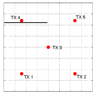
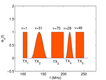
Figure 2: (left) Position of sources and obstructing wall; (right) PSD generated by the active transmitters.

Consider a set of $N_{r}=100$ CRs uniformly distributed in an area of $1{\rm Km}^{2}$, cooperating to estimate the PSD map generated by $N_{s}=5$ licensed users (sources) located as in Fig. 2 (left). The five transmitted signals are raised cosine pulses with roll-off factors $\rho\in\{0,1\}$, and bandwidths $W\in\{10,20,30\}$ MHz. They share the frequency band $B=[100,260]$ MHz with spectra centered at frequencies $f_{c}=105,\ 140,\ 185,\ 215,$ and $240$ MHz, respectively. Fig. 2 (right) depicts the PSD generated by the active transmitters.

The PSD generated by source $s$ experiences fading and shadowing effects in its propagation from $\mathbf{x}_{s}$ to any location $\mathbf{x}$, where it can be measured in the presence of noise. A 6-tap Rayleigh model is adopted for the multipath channel $H_{s}(f,\tau,\mathbf{x})$ between $\mathbf{x}_{s}$ and $\mathbf{x}$, whose expected gain adheres to the path-loss law $E(|H_{s}|^{2})=\exp(-||\mathbf{x}_{s}-\mathbf{x}||_{2}^{2}/\Delta^{2})$, with $\Delta=0.8$. A deterministic shadowing effect is generated by a $18$m-high and $500$m-wide wall represented by the black segment in Fig. 2 (left). It produces a knife-edge effect on the power emitted by the antennas at a height of $20$m. The simulated tests presented here account for the shadowing at ground level.

VI-A Spectrum cartography

When designing the basis functions in (1), it is known a priori that the transmitted signals are indeed normalized raised cosine pulses with roll-off factors $\rho\in\{0,1\}$, and bandwidths $W\in\{10,20,30\}$ MHz. However, the actual combination of bandwidths and roll-off factors used can be unknown, which justifies why an overcomplete set of bases becomes handy. Transmitted signals with bandwidth $W=10$ MHz are searched over a grid of $16$ evenly spaced center frequencies $f_{c}$ in $B$. Likewise, for $W=20$ and $30$ MHz, $15$ and $14$ center frequencies are considered, respectively. This amounts to $2\times(16+15+14)=90$ possible combinations for $\rho$, $W$, and $f_{c}$, thus $N_{b}=90$ bases are adopted.

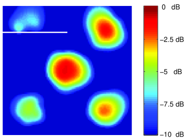
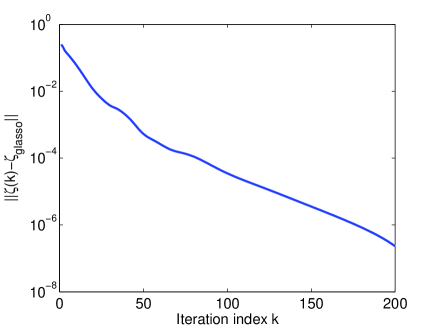
Figure 3: (left) Aggregate map estimate in dB; (right) error evolution of the GLasso updates

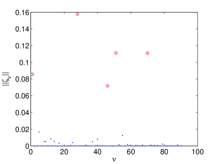
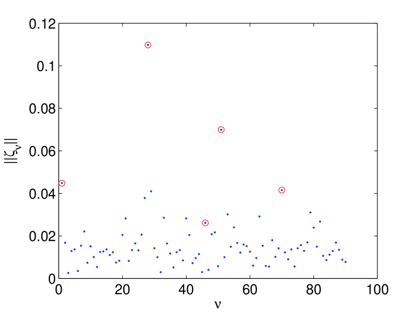
Figure 4: (left) Frequency bases selected by the group-Lassoed spline-based estimator; (right) and by ridge regression.

Each CR computes periodogram samples $\hat{\phi}_{rn}(\tau)$ at $N=64$ frequencies with $SNR=-5$ dB, and averages them across $T=100$ time-slots to form $\varphi_{rn},\ n=1,\ldots,64$ as in (3). These network-wide observations at $T=100$ are collected in $\bm{\varphi}$, and following steps S1-S4 at the end of Section IV, the spline-based estimator (12), and thus the PSD map $\hat{\Phi}(\mathbf{x},f)$ is formed. This map is summed across frequencies, and the result is shown in Fig. 3 (left) which depicts the positions of transmitting CRs, as well as the radially-decaying spectra of four of them (those not affected by the obstacle). It also identifies the effect of the wall by “flattening” the spectrum emitted by the fifth source at the top-left corner. Inspection of the estimate $\hat{\Phi}(\mathbf{x},f)$ across frequency confirms that group-Lasso succeeds in selecting the candidate bases. Fig. 4 (left) shows points representing $\|\hat{\bm{\zeta}}_{\nu}\|_{2}$, $\nu=1,\ldots,N_{b}$, where $\hat{\bm{\zeta}}_{\nu}$ is the sub-vector in the solution of the group-Lasso estimator (13) associated with $g_{\nu}(\mathbf{x})$ and $b_{\nu}(f)$. They peak at indexes $\nu=1,\ 28,\ 46,\ 51,$ and $70$ (circled in red), which correspond to the “ground-truth” model, since bases $b_{1},\ b_{28},\ b_{46},\ b_{51},$ and $b_{70}$ match the spectra of the transmitted signals. Even though approximately 75% of the variables drop out of the model, some spurious coefficients are retained and their norms are markedly smaller than those of the “ground-truth” bases. This is expected because based on finite samples there is no guarantee that group-Lasso will recover the exact support, in general. Nevertheless, the effectiveness of group-Lasso in revealing the transmitted bases is apparent when compared to other regularization alternatives. Fig. 4 (right) depicts the counterpart of Fig. 4 (left) when using a sparsity-agnostic ridge regression scheme instead of (13). In this case, no basis selection takes place, and the spurious factors are magnified up to a level comparable to three of the “true” basis function $b_{\nu}(f)$. To the best of our knowledge, no other basis selection methods in the literature are applicable to the nonparametric model (1) considered here. In particular, COSSO in [16] is not applicable since it does not provide a basis selection method and relies on orthogonality assumptions.

In summary, this test case demonstrates that the spline-based estimator can reveal which frequency bands are (un)occupied at each point in space, thus allowing for spatial reuse of the idle bands. For instance, transmitter $\textrm{TX}_{5}$ at the top-right corner is associated with the basis function $b_{46}(f)$, the only one of the transmitted five that occupies the $230-260$ MHz sub-band. Therefore, this sub-band can be reused at locations $\mathbf{x}$ away from the transmission range of $\textrm{TX}_{5}$, which is revealed in Fig. 3 (left).

The group-Lasso estimator in S1 was obtained via the GLasso algorithm developed in Section V (cf. Algorithm 2). The GLasso output at iteration $k=1,000$ is compared to previous iterates $\bm{\zeta}(k)$ in Fig. 3 (right), which demonstrates the monotone decay of their difference, and thus corroborates convergence to a limit point. Then, it is verified numerically that $\bm{\zeta}(1000)$ satisfies the necessary and sufficient conditions for optimality of (19), as given in [29]. These two tests together provide numerical confirmation of Proposition V-B on the convergence of GLasso, and the optimality of the limit point.

VI-B Tuning parameters via cross-validation

Results in Figs. 3 (left) and 4 depend on the judicious selection of parameters $\lambda$ and $\mu$ in (12). Parameter $\lambda$ affects smoothness, which translates to congruence among PSD samples, allowing the CRs to recover the radial aspect of the transmit-power. Parameter $\mu$ controls the sparsity in the solution, which dictates the number of bases, and thus transmission schemes that the estimator considers active.

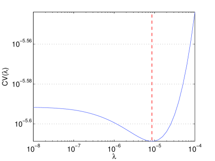
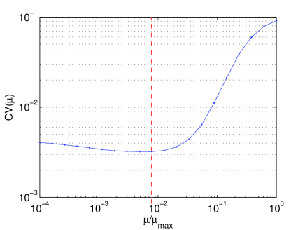
Figure 5: (left) Minimization of the CV error over $\lambda$; (right) and over $\mu$.

To select $\lambda$ and $\mu$ jointly so that both smoothness and sparsity are properly accounted for, one could consider a two-dimensional grid of candidate pairs, and minimize the CV error over this grid. However, this is computationally demanding, especially because the nondifferentiable cost in (13) renders the shortcuts in Appendix D not applicable (see also Remark IV-A). A three-step alternative is followed here. First, estimator (12) is obtained using an arbitrarily small value of $\lambda=1\times 10^{-6}$, and selecting $\mu=0.1\mu_{\max}$, where $\mu_{\max}$ is given in subsection IV-A. In the second step, only the surviving bases are kept, and the sparsifying penalty is no longer considered, thus reducing the estimator to that of Section III. If the reduced matrix $\mathbf{B}$, built from the surviving bases, is full rank (otherwise repeat the first step with a larger value of $\mu$), the procedure in Appendix D is followed to adjust the value of $\lambda$ via leave-one-out CV. The result of this step is illustrated in Fig. 5 (left), where the minimizer $\lambda_{CV}=7.9433\times 10^{-6}$ of the OCV cost is selected. The final step consists of reconsidering the sparsity enforcing penalty in (12), and selecting $\mu$ using $5$-fold CV. The minimizer of the CV error $\mu_{CV}=0.0078\mu_{\max}$ corresponding to this step is depicted in Fig. 5 (right). Using the $\lambda_{CV}$ and $\mu_{CV}$ so obtained, the PSD map plotted in Fig. 3 (left) was constructed. The rationale behind this approach is that it corresponds to a single step of a coordinate descent algorithm for minimizing the CV error $CV(\lambda,\mu)$. Function $CV(\lambda,\mu)$ is typically unimodal, with much higher sensitivity on $\mu$ than on $\lambda$, a geometric feature leading the first coordinate descent update to be close to the optimum.

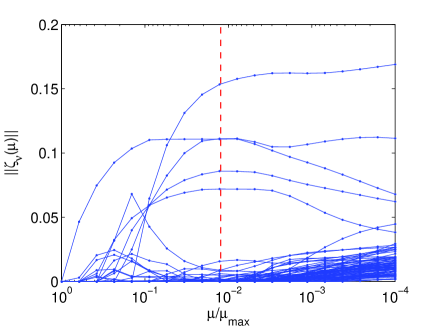
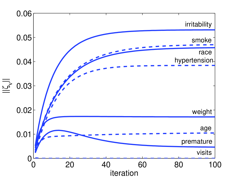
Figure 6: (left) Group-Lasso path of solutions $\|\bm{\zeta}_{\nu}\|_{2}$ as $\mu$ varies; (right) factors affecting birthweight, evolution of GLasso iterates.

The importance of an appropriate $\mu$ value becomes evident when inspecting how many bases are retained by the estimator as $\mu$ decreases from $\mu_{\max}$ to $1\times 10^{-4}\mu_{\max}$. The $N_{b}$ lines in Fig. 6 (left) link points representing $\|\hat{\bm{\zeta}}_{\nu}(\mu)\|_{2}$, as $\mu$ takes on $20$ evenly spaced values on a logarithmic scale, comprising the so-termed group-Lasso path of solutions. When $\mu=\mu_{\max}$ is selected, by definition the estimator forces all $\hat{\bm{\zeta}}_{\nu}$ to zero, thus discarding all bases. As $\mu$ tends to zero all bases become relevant and eventually enter the model, which confirms the premise that LS estimators suffer from overfitting when the underlying model is overcomplete. The cross-validated value $\mu_{CV}$ is indicated with a dashed vertical line that crosses the path of solutions at the values of $\|\hat{\bm{\zeta}}_{\nu}\|_{2}$. At this point, five sub-vectors corresponding to the factors $\nu=1,\ 28,\ 46,\ 51,$ and $70$ are considerably far away from zero hence showing strong effects, in par with the results depicted in Fig. 4 (left). Certainly interesting would be to corroborate the effectiveness of the proposed PSD map estimator on real data comprising spatially distributed RF measurements. Upon availability of such dataset, this direction will be pursued and reported elsewhere.

VI-C Example with real data

The goal of this section is to demonstrate that the GLasso algorithm in Section V can be useful for applications other than the spline-based BEM for spectrum cartography dealt with in Sections III and IV. This demonstration will rely on the birthweight dataset from [14], considered also by the seminal group-Lasso work of [29]. The objective is to predict the human birthweight from $p=8$ factors including the mother’s age, weight, race, smoke habits, number of previous premature labors, history of hypertension, uterine irritability, and number of physician visits during the first trimester of pregnancy. Third-order polynomials were considered to model nonlinear effects of the age and weight on the response, augmenting the model size to $p=12$ by grouping the polynomial coefficients in two subsets of three variables.

GLasso is run under this setup, over the set of $N=189$ samples, with $\mu$ selected via 7-fold CV. Fig. 6 (right) depicts the evolution of the factors’ strength measured by $\|\zeta_{\nu}\|_{2}^{2}$, which – as expected – converge to the same prediction model as in [29]. Additionally, GLasso is capable of determining that the eighth factor (visits) is not significant even from the first iterations, allowing for early model selection.

VII Concluding Summary

A basis expansion approach was introduced in this paper to estimate a multi-dimensional field, whose dependence on a subset of its variables is modeled through preselected (and generally overlapping) basis functions weighted by unknown coefficient-functions of the remaining variables. The unknown coefficient functions can be estimated from the field’s noisy samples, by solving a variational LS problem which admits infinite solutions. Without extra constraints, the estimated field interpolates perfectly the data samples, at the price of severely overfitting the true field elsewhere. The first contribution was to regularize this variational LS cost by a smoothing term, which can afford a unique finite-parameter spline-based solution. The latter is expressed in terms of radial kernels and polynomials whose parameters were estimated in closed form. A recursive PSD tracker was also developed for slowly time-varying spectra.

The second main contribution pertains to a robust variant of the function estimator, when an overcomplete set of bases is adopted to effectively accommodate model uncertainties. The novel estimator here minimizes the variational LS cost regularized by a term that performs basis selection, and thus yields a parsimonious description of the field by retaining those few members of the basis that “better” explain the data. This attribute is achieved because the added penalty induces a group (G)Lasso estimator on the parameters of the kernels and polynomials. Even though the number of unknowns increases with overcomplete bases, most coefficients are zero, meaning that the complexity remains at an affordable level using the sparsity-promoting GLasso. Notwithstanding, (group-) Lasso here is introduced to effect (group-) sparsity in the space of smooth functions.

The third contribution is a provably convergent GLasso estimator developed based on AD-MoM iterations. It entails parallel closed-form updates, which involve simple vector soft-thresholding operations per factor. Its fully-distributed counterpart was also developed for use by a network of wireless sensors, or, multiple processors to balance the load of a computational cluster. It is worth stressing that both GLassso and DGLasso are standalone tools for sparse linear regression, applicable to a gamut of problems that go beyond the field estimation context of this paper.

The fourth contribution is in the context of wireless CR network sensing (our overarching practical motivation), where the overcomplete estimated field enables cartographing the space-frequency distribution of power generated by RF sources whose transmit-PSDs are shaped by, e.g., raised-cosine pulses with possibly different roll-off factors, center frequencies, and bandwidths. Using periodogram samples collected by spatially distributed CRs, the sparsity-aware spline-based estimator yields an atlas of PSD maps (one map per frequency). As corroborated by simulations, the atlas enables localizing the sources and discerning their transmission parameters, even in the presence of frequency-selective Rayleigh fading and pronounced shadowing effects due to e.g., an obstructing wall. Simulated tests also illustrated the convergence of Glasso, and confirmed that the sparsity-promoting regularization is effective in selecting those basis functions that strongly influence the field, when the tuning parameters are cross-validated properly.

Given the existing connections between splines and classical estimators for both random and deterministic field models, the spline-based methods developed in this paper provide a unifying framework suitable for both paradigms. The model and the resultant (parsimonious) estimates can thus be used in more general statistical inference and localization problems, whenever the data admit a basis expansion over a proper subset of its dimensions. Furthermore, results in this paper extend to kernels other than radial basis functions, whenever the smoothing penalty is replaced by a norm induced from an RKHS. Also of interest is to quantify the number of data required to attain a prescribed approximation error, in light of the existing connections between spline-based reconstruction and Shannon’s sampling theory [25].

Acnowledgments

The authors would like to thank Prof. Hui Zou (School of Statistics, University of Minnesota) for his feedback which improved the exposition of ideas in this paper.

A. Proof of Proposition III-A: Rewrite (4) as

$$\min_{\{g_{\nu}\in\mathcal{S}\}_{\nu=2}^{N_{b}}}\left[\min_{g_{1}\in\mathcal{S}}\sum_{r=1}^{N_{r}}\sum_{n=1}^{N}\left(\varphi_{rn}^{(-1)}-g_{1}(\mathbf{x}_{r})b_{1}(f_{n})\right)^{2}+\lambda\int_{\mathbb{R}^{2}}||\nabla^{2}g_{1}(\mathbf{x})||_{F}^{2}d\mathbf{x}\right]+\lambda\sum_{\nu=2}^{N_{b}}\int_{\mathbb{R}^{2}}||\nabla^{2}g_{\nu}(\mathbf{x})||_{F}^{2}d\mathbf{x}$$ (36)

with $\varphi_{rn}^{(-1)}:=\varphi_{rn}-\sum_{\nu=2}^{N_{b}}g_{\nu}(\mathbf{x}_{r})b_{\nu}(f_{n})$. Focusing on the inner minimization w.r.t. $g_{1}$, fix the set of functions $\{g_{\nu}\}_{\nu=2}^{N_{b}}$, and note that only the first two terms are relevant (those within the square brackets). It follows from [10, Theorem 4 bis] that $\hat{g}_{1}$ takes the form in (5), with coefficients $\bm{\beta}_{1},\bm{\alpha}_{11}$ and $\alpha_{10}$ that depend on $G^{(-1)}:=\{g_{\nu}(x_{r}),\ r=1,\ldots,N_{r},\ \nu=2,\ldots,N_{b}\}$ through $\varphi_{rn}^{(-1)}$. The next step is to minimize (36) w.r.t. $g_{2}$ but with $\{g_{\nu}\}_{\nu=3}^{N_{b}}$ fixed, which amounts to

$$\min_{g_{2}\in\mathcal{S}}\sum_{r=1}^{N_{r}}\sum_{n=1}^{N}\left(\varphi_{rn}^{(-2)}-\hat{g}_{1}(\mathbf{x}_{r})b_{1}(f_{n})-g_{2}(\mathbf{x}_{r})b_{2}(f_{n})\right)^{2}+\lambda\int_{\mathbb{R}^{2}}||\nabla^{2}\hat{g}_{1}(\mathbf{x})||_{F}^{2}d\mathbf{x}+\lambda\int_{\mathbb{R}^{2}}||\nabla^{2}g_{2}(\mathbf{x})||_{F}^{2}d\mathbf{x}$$ (37)

where $\varphi_{rn}^{(-2)}:=\varphi_{rn}-\sum_{\nu=3}^{N_{b}}g_{\nu}(\mathbf{x}_{r})b_{\nu}(f_{n})$. In the first two summands of the cost in (37), $\hat{g}_{1}$ depends on $g_{2}$ via $G^{(-1)}$. Because $G^{(-1)}$ only involves evaluating $g_{2}$ on $\mathcal{X}$, [10, Theorem 4 bis] can be applied again, and the optimal solution $\hat{g}_{2}$ takes the from (5). The same argument carries over to subsequent minimization steps for $\nu=3,\ldots,N_{b}$, establishing that all $\{\hat{g}_{\nu}(\mathbf{x})\}$ are thin-plate splines as in (5).

B. Proof of (6)-(8): Upon substituting (5) into (4), it will shown next that the optimal coefficients $\{\hat{\bm{\alpha}},\hat{\bm{\beta}}\}$ specifying $\{\hat{g}_{\nu}(\mathbf{x})\}_{\nu=1}^{N_{b}}$ are obtained as solutions to the following constrained, regularized LS problem

$$\min_{\bm{\alpha},\bm{\beta}}\frac{1}{{N_{r}N}}\left\|\bm{\varphi}-(\mathbf{B}\otimes\mathbf{K})\bm{\beta}-(\mathbf{B}\otimes\mathbf{T})\bm{\alpha}\right\|_{2}^{2}+\lambda\bm{\beta}^{\prime}(\mathbf{I}_{N_{b}}\otimes\mathbf{K})\bm{\beta}$$

$${\quad}\mbox{s. t.}{\quad}(\mathbf{I}_{N_{b}}\otimes\mathbf{T}^{\prime})\bm{\beta}=\mathbf{0}_{3N_{b}}.$$ (38)

Observe first that the constraints $\bm{\beta}_{\nu}\in\mathcal{B}$ in Proposition 1 can be expressed as $\mathbf{T}^{\prime}\bm{\beta}_{\nu}=\mathbf{0}_{3}$ for each $\nu=1,\ldots,N_{b}$, or jointly as $(\mathbf{I}_{N_{b}}\otimes\mathbf{T}^{\prime})\bm{\beta}=\mathbf{0}_{3N_{b}}$. For the optimization objective in (Acnowledgments), note from (5) that $\hat{g}_{\nu}(\mathbf{x}_{r})=\mathbf{k}_{r}^{\prime}\bm{\beta}_{\nu}+\mathbf{t}_{r}^{\prime}\bm{\alpha}_{\nu}$, where $\mathbf{k}_{r}^{\prime}$ and $\mathbf{t}_{r}^{\prime}$ are the $r$th rows of $\mathbf{K}$ and $\mathbf{T}$, respectively. The first term in the cost of (4) can be expressed (up to a factor $({N_{r}N})^{-1}$) as

$$\sum_{n=1}^{N}\sum_{r=1}^{N_{r}}\left(\varphi_{rn}-\sum_{\nu=1}^{N_{b}}b_{\nu}(f_{n})[\mathbf{k}_{r}^{\prime}\bm{\beta}_{\nu}+\mathbf{t}_{r}^{\prime}\bm{\alpha}_{\nu}]\right)^{2} = \sum_{n=1}^{N}\sum_{r=1}^{N_{r}}\left(\varphi_{rn}-(\mathbf{b}_{n}\otimes\mathbf{k}_{r})^{\prime}\bm{\beta}-(\mathbf{b}_{n}\otimes\mathbf{t}_{r})^{\prime}\bm{\alpha}\right)^{2}$$

$$= \sum_{n=1}^{N}\left\|\bm{\varphi}_{n}-(\mathbf{b}_{n}^{\prime}\otimes\mathbf{K})\bm{\beta}-(\mathbf{b}_{n}^{\prime}\otimes\mathbf{T})\bm{\alpha}\right\|_{2}^{2}$$

$$= \left\|\bm{\varphi}-(\mathbf{B}\otimes\mathbf{K})\bm{\beta}-(\mathbf{B}\otimes\mathbf{T})\bm{\alpha}\right\|_{2}^{2}.$$

Consider next the penalty term in the cost of (4). Substituting into (5), it follows that $\int_{\mathbb{R}^{2}}||\nabla^{2}\hat{g}_{\nu}(\mathbf{x})||_{F}^{2}d\mathbf{x}=\bm{\beta}_{\nu}^{\prime}\mathbf{K}\bm{\beta}_{\nu}$  [26, p. 33]. It thus holds that

$$\lambda\sum_{\nu=1}^{N_{b}}\int_{\mathbb{R}^{2}}||\nabla^{2}\hat{g}_{\nu}(\mathbf{x})||_{F}^{2}d\mathbf{x}=\lambda\sum_{\nu=1}^{N_{b}}\bm{\beta}_{\nu}^{\prime}\mathbf{K}\bm{\beta}_{\nu}=\lambda\bm{\beta}^{\prime}(\mathbf{I}_{N_{b}}\otimes\mathbf{K})\bm{\beta}$$

from which (Acnowledgments) follows readily.

Now that the equivalence between (4) and (Acnowledgments) has been established, the latter must be solved for $\bm{\alpha}$ and $\bm{\beta}$. Even though $\mathbf{K}$ (hence $\mathbf{I}_{N_{b}}\otimes\mathbf{K}$) is not positive definite, it is still possible to show that $\bm{\beta}^{\prime}(\mathbf{I}_{N_{b}}\otimes\mathbf{K})\bm{\beta}>0$ for any $\bm{\beta}$ such that $(\mathbf{I}_{N_{b}}\otimes\mathbf{T}^{\prime})\bm{\beta}=\mathbf{0}_{3N_{b}}$ [10, p. 85], implying that (Acnowledgments) is convex. Proceeding along the lines of [26, p. 33], note first that the constraint $(\mathbf{I}_{N_{b}}\otimes\mathbf{T}^{\prime})\bm{\beta}=\mathbf{0}_{3N_{b}}$ implies the existence of a vector $\bm{\gamma}\in\mathbb{R}^{N_{b}(N_{r}-3)}$ satisfying (8). After this change of variables, (Acnowledgments) is transformed into an unconstrained quadratic program, which can be solved in closed form for $\{{\bm{\alpha}},{\bm{\gamma}}\}$. Hence, setting both gradients w.r.t. ${\bm{\alpha}}$ and ${\bm{\gamma}}\}$ to zero yields (6) and (7).

C. Proof of Proposition IV-A: After substituting (17) into (12), one finds the optimal $\{{\bm{\alpha}},{\bm{\beta}}\}$ specifying $\{\hat{g}_{\nu}(\mathbf{x})\}_{\nu=1}^{N_{b}}$ in (17), as solutions to the following constrained, regularized LS problem

$$\min_{\bm{\alpha},\bm{\beta}}\frac{1}{{N_{r}N}}\left\|\bm{\varphi}-(\mathbf{B}\otimes\mathbf{K})\bm{\beta}-(\mathbf{B}\otimes\mathbf{T})\bm{\alpha}\right\|_{2}^{2}+\lambda\bm{\beta}^{\prime}(\mathbf{I}_{N_{b}}\otimes\mathbf{K})\bm{\beta}+\mu\sum_{\nu=1}^{N_{b}}\|\mathbf{K}\bm{\beta}_{\nu}+\mathbf{T}\bm{\alpha}_{\nu}\|_{2}$$

$${\quad}\mbox{s. t.}{\quad}(\mathbf{I}_{N_{b}}\otimes\mathbf{T}^{\prime})\bm{\beta}=\mathbf{0}_{3N_{b}}.$$ (39)

With reference to (Acnowledgments), consider grouping and reordering the variables $\{\bm{\alpha},\bm{\beta}\}$ in the vector $\mathbf{u}:=[\mathbf{u}_{1}^{\prime},\ldots,\mathbf{u}_{N_{b}}^{\prime}]^{\prime}$, where $\mathbf{u}_{\nu}:=[\bm{\beta}_{\nu}^{\prime}\>\>\bm{\alpha}_{\nu}^{\prime}]^{\prime}$. As argued in Section III-A, the constraints $\mathbf{T}^{\prime}\bm{\beta}_{\nu}=\mathbf{0}$ can be eliminated through the change of variables $\mathbf{u}_{\nu}=\textrm{bdiag}(\mathbf{Q}_{2},\mathbf{I}_{3})\mathbf{v}_{\nu}$ for $\nu=1,\ldots,N_{b}$; or compactly as $\mathbf{u}=(\mathbf{I}_{N_{b}}\otimes\textrm{bdiag}(\mathbf{Q}_{2},\mathbf{I}_{3}))\mathbf{v}$. The next step is to express the three summands in the cost of (Acnowledgments) in terms of the new vector optimization variable $\mathbf{v}$. Noting that $\mathbf{k}_{r}^{\prime}\bm{\beta}_{\nu}+\mathbf{t}_{r}^{\prime}\bm{\alpha}_{\nu}=[\mathbf{k}_{r}^{\prime}\>\>\mathbf{t}_{r}^{\prime}]\mathbf{u}_{\nu}$, and mimicking the steps in Appendix A, the first summand is

$$\frac{1}{{N_{r}N}}\left\|\bm{\varphi}-(\mathbf{B}\otimes\mathbf{K})\bm{\beta}-(\mathbf{B}\otimes\mathbf{T})\bm{\alpha}\right\|_{2}^{2}= \>\frac{1}{{N_{r}N}}\left\|\bm{\varphi}-(\mathbf{B}\otimes[\mathbf{K}\>\>\mathbf{T}])\mathbf{u}\right\|_{2}^{2}$$

$$= \>\frac{1}{{N_{r}N}}\left\|\bm{\varphi}-(\mathbf{B}\otimes[\mathbf{KQ}_{2}\>\>\mathbf{T}])\mathbf{v}\right\|_{2}^{2}.$$ (40)

The second summand due to the thin-plate penalty can be expressed as

$$\lambda\sum_{\nu=1}^{N_{b}}\bm{\beta}_{\nu}^{\prime}\mathbf{K}\bm{\beta}_{\nu}= \>\lambda\sum_{\nu=1}^{N_{b}}\mathbf{u}_{\nu}^{\prime}\textrm{bdiag}(\mathbf{K},\mathbf{0})\mathbf{u}_{\nu}=\lambda\sum_{\nu=1}^{N_{b}}\mathbf{v}_{\nu}^{\prime}\textrm{bdiag}(\mathbf{Q}_{2}^{\prime}\mathbf{K}\mathbf{Q}_{2},\mathbf{0})\mathbf{v}_{\nu}$$

$$= \>\lambda\mathbf{v}^{\prime}(\mathbf{I}_{N_{b}}\otimes\textrm{bdiag}(\mathbf{Q}_{2}^{\prime}\mathbf{K}\mathbf{Q}_{2},\mathbf{0}))\mathbf{v}$$ (41)

while the last term is $\mu\sum_{\nu=1}^{N_{b}}\|\mathbf{K}\bm{\beta}_{\nu}+\mathbf{T}\bm{\alpha}_{\nu}\|_{2}=\mu\sum_{\nu=1}^{N_{b}}\|[\mathbf{K}\>\>\mathbf{T}]\mathbf{u}_{\nu}\|_{2}=\mu\sum_{\nu=1}^{N_{b}}\|[\mathbf{KQ}_{2}\>\>\mathbf{T}]\mathbf{v}_{\nu}\|_{2}.$ Combining (Acnowledgments) with (Acnowledgments) by completing the squares, problem (Acnowledgments) is equivalent to

$$\min_{\mathbf{v}}\frac{1}{N_{r}N}\left\|\left[\begin{array}[]{c}\bm{\varphi}\\ \mathbf{0}\end{array}\right]-\left[\begin{array}[]{c}\mathbf{B}\otimes[\mathbf{KQ}_{2}\>\>\mathbf{T}]\\ \mathbf{I}_{N_{b}}\otimes\textrm{bdiag}(({N_{r}N}\lambda\mathbf{Q}_{2}^{\prime}\mathbf{K}\mathbf{Q}_{2})^{1/2},\mathbf{0})\end{array}\right]\mathbf{v}\right\|_{2}^{2}+\mu\sum_{\nu=1}^{N_{b}}\|[\mathbf{KQ}_{2}\>\>\mathbf{T}]\mathbf{v}_{\nu}\|_{2}$$ (42)

and becomes (13) under the identities (16), and after the change of variables $\bm{\zeta}:=[\bm{\zeta}_{1}^{\prime},\ldots,\bm{\zeta}_{N_{b}}^{\prime}]^{\prime}=(\mathbf{I}_{N_{b}}\otimes[\mathbf{KQ}_{2}\>\>\mathbf{T}])\mathbf{v}$. By definition of $\mathbf{u}$, $\mathbf{v}$, and $\bm{\zeta}$, the original variables can be recovered through the transformation in (18).

D. Selection of the smoothing parameter in (4): The method to be developed builds on the so-termed leave-one-out CV, which proceeds as follows; see e.g., [26, Ch. 4]. Consider removing a single data point $\varphi_{rn}$ from the collection of ${N_{r}N}$ measurements available to the sensing radios. For a given $\lambda$, let $\hat{\Phi}^{(-rn)}_{\lambda}(\mathbf{x},f)$ denote the leave-one-out estimated PSD map, obtained by solving (4) following steps S1-S3 in Section III-A, using the ${N_{r}N}-1$ remaining data points. The aforementioned estimation procedure is repeated $N_{r}N$ times by leaving out each of the data points $\varphi_{rn},$ $r=1,\ldots,N_{r}$ and $n=1,\ldots,N$, one at a time. The leave-one-out or ordinary CV (OCV) [13, p. 242], [26, p. 47], for the problem at hand is given by

$$\textrm{OCV}(\lambda)=\frac{1}{{N_{r}N}}\sum_{r=1}^{N_{r}}\sum_{n=1}^{N}\left(\varphi_{rn}-\hat{\Phi}^{(-rn)}_{\lambda}(\mathbf{x}_{r},f_{n})\right)^{2}$$ (43)

while the optimum $\lambda$ is selected as the minimizer of $\textrm{OCV}(\lambda)$, over a grid of values $\lambda\in[0,\lambda_{\max}]$. Function (43) constitutes an average of the squared prediction errors over all data points; hence, its minimization offers a natural criterion. The method is quite computationally demanding though, since the system of linear equations (6)-(8) has to be solved $N_{r}N$ times for each value of $\lambda$ on the grid. Fortunately, this computational burden can be significantly reduced for the spline-based PSD map estimator considered here.

Recall the vector $\bm{\varphi}$ collecting all data points measured at locations $\mathcal{X}$ and frequencies $\mathcal{F}$. Define next a similar vector $\hat{\bm{\varphi}}$ containing the respective predicted values at the given locations and frequencies, which is obtained after solving (4) with all the data in $\bm{\varphi}$ and a given value of $\lambda$. The following lemma establishes that the PSD map estimator is a linear smoother, which means that the predicted values are linearly related to the measurements, i.e., $\hat{\bm{\varphi}}=\mathbf{S}_{\lambda}\bm{\varphi}$ for a $\lambda$-dependent matrix $\mathbf{S}_{\lambda}$ to be determined. Common examples of linear smoothers are ridge regressors and smoothing splines; further details are in [13, p. 153]. For linear smoothers, by virtue of the leave-one-out lemma [26, p. 50] it is possible to rewrite (43) as

$$\textrm{OCV}(\lambda)=\frac{1}{{N_{r}N}}\sum_{r=1}^{N_{r}}\sum_{n=1}^{N}\left(\frac{\varphi_{rn}-\hat{\Phi}_{\lambda}(\mathbf{x}_{r},f_{n})}{1-[\mathbf{S}_{\lambda}]_{ii}}\right)^{2}$$ (44)

where $\hat{\Phi}_{\lambda}(\mathbf{x},f)$ stands for the estimated PSD map when all data in $\bm{\varphi}$ are utilized in (4). The beauty of the leave-one-out lemma stems from the fact that given $\lambda$ and the main diagonal of matrix $\mathbf{S}_{\lambda}$, the right-hand side of (44) indicates that fitting a single model (rather than $N_{r}N$ of them) suffices to evaluate $\textrm{OCV}(\lambda)$. The promised lemma stated next specifies the value of $\mathbf{S}_{\lambda}$ necessary to evaluate (44).

Lemma 3: The PSD map estimator in (4) is a linear smoother, with smoothing matrix given by

$$\mathbf{S}_{\lambda}= \>(\mathbf{B}\otimes\{\mathbf{KQ}_{2}-\mathbf{TR}^{-1}\mathbf{Q}_{1}^{\prime}\mathbf{KQ}_{2}\})[(\mathbf{B}^{\prime}\mathbf{B}\otimes\mathbf{Q}_{2}^{\prime}\mathbf{K}\mathbf{Q}_{2})+{N_{r}N}\lambda\mathbf{I}]^{-1}(\mathbf{B}^{\prime}\otimes\mathbf{Q}_{2}^{\prime})$$

$$\>+(\mathbf{B}\bm{\Gamma}^{-1}\bm{\Omega}_{1}^{-1}\otimes\mathbf{TR}^{-1}\mathbf{Q}_{1}^{\prime}).$$ (45)

Proof:

Reproduce the structure of $\bm{\varphi}$ in Section III-A to form the supervector $\hat{\bm{\varphi}}:=[\hat{\bm{\varphi}}_{1}^{\prime},\ldots,\hat{\bm{\varphi}}_{N}^{\prime}]^{\prime}\in\mathbb{R}^{{N_{r}N}}$, by stacking each vector $\hat{\bm{\varphi}}_{n}:=[\hat{\Phi}_{\lambda}(\mathbf{x}_{1},f_{n}),\ldots,\hat{\Phi}_{\lambda}(\mathbf{x}_{N_{r}},f_{n})]^{\prime}$ corresponding to the spatial PSD predictions at frequency $f_{n}\in\mathcal{F}$. From (5), it follows that $\hat{\Phi}_{\lambda}(\mathbf{x}_{r},f_{n})=(\mathbf{b}_{n}\otimes\mathbf{k}_{r})^{\prime}\hat{\bm{\beta}}-(\mathbf{b}_{n}\otimes\mathbf{t}_{r})^{\prime}\hat{\bm{\alpha}}$, where $\mathbf{b}_{n}^{\prime}$, $\mathbf{k}_{r}^{\prime}$ and $\mathbf{t}_{r}^{\prime}$ are the $n$th and $r$th rows of $\mathbf{B}$, $\mathbf{K}$ and $\mathbf{T}$, respectively. By stacking the PSD map estimates, it follows that $\hat{\bm{\varphi}}_{n}=(\mathbf{b}_{n}^{\prime}\otimes\mathbf{K})\hat{\bm{\beta}}-(\mathbf{b}_{n}^{\prime}\otimes\mathbf{T})\hat{\bm{\alpha}},$ which readily yields

$$\hat{\bm{\varphi}}=(\mathbf{B}\otimes\mathbf{K})\hat{\bm{\beta}}-(\mathbf{B}\otimes\mathbf{T})\hat{\bm{\alpha}}.$$ (46)

Because the estimates $\{\hat{\bm{\alpha}},\hat{\bm{\beta}}\}$ are linearly related to the measurements $\bm{\varphi}$ [cf. (6)-(8)], so is $\hat{\bm{\varphi}}$ as per (46), establishing that the PSD map estimator in (4) is indeed a linear smoother. Next, solve explicitly for $\{\hat{\bm{\alpha}},\hat{\bm{\beta}}\}$ in (6)-(8) and substitute the results in (46), to unveil the structure of the smoothing matrix $\mathbf{S}_{\lambda}$ such that $\hat{\bm{\varphi}}=\mathbf{S}_{\lambda}\bm{\varphi}$. Simple algebraic manipulations lead to the expression (Acnowledgments). ∎

The effectiveness of the leave-one-out CV approach is corroborated via simulations in Section VI.

E. Proof of (31)-(34): Recall the augmented Lagrangian function in (V-B), and let $\bm{\zeta}:=\{\bm{\zeta}_{r}\}_{r\in{\cal R}}$ for notational brevity. When used to solve (26), the three steps in the AD-MoM are given by:

[S1]

Local estimate updates:

$$\bm{\zeta}(k+1)=\mbox{arg}\>\min_{\bm{\zeta}}{\mathcal{L}}_{c}\left[\bm{\zeta},\bm{\gamma}(k),\bm{{\mathit{v}}}(k)\right].$$ (47)

[S2]

Auxiliary variable updates:

$$\bm{\gamma}(k+1)=\mbox{arg}\min_{\bm{\gamma}}{\mathcal{L}}_{c}\left[\bm{\zeta}(k+1),\bm{\gamma},\bm{{\mathit{v}}}(k)\right].$$ (48)

[S3]

Multiplier updates:

$${\mathbf{v}}_{r}(k+1) ={\mathbf{v}}_{r}(k)+c[\bm{\zeta}_{r}(k+1)-\bm{\gamma}_{r}(k+1)]$$ (49)

$$\breve{\mathbf{v}}_{r}^{r^{\prime}}(k+1) =\breve{\mathbf{v}}_{r}^{r^{\prime}}(k)+c[\bm{\zeta}_{r}(k+1)-{\bm{\gamma}}_{r}^{r^{\prime}}(k+1)]$$ (50)

$$\bar{{\mathbf{v}}}_{r}^{r^{\prime}}(k+1) =\bar{{\mathbf{v}}}_{r}^{r^{\prime}}(k)+c[\bm{\zeta}_{r^{\prime}}(k+1)-{\bm{\gamma}}_{r}^{r^{\prime}}(k+1)].$$ (51)

Focusing first on [S2], observe that (V-B) is separable across the collection of variables $\{\bm{\gamma}_{j}\}$ and $\{{\bm{\gamma}}_{r}^{r^{\prime}}\}$ that comprise $\bm{\gamma}$. The minimization w.r.t. the latter group reduces to

$${\bm{\gamma}}_{r}^{r^{\prime}}(k+1) =\arg\min_{{\bm{\gamma}}_{r}^{r^{\prime}}}c\|{\bm{\gamma}}_{r}^{r^{\prime}}\|^{2}-c\Big{(}\bm{\zeta}_{r}(k+1)+\bm{\zeta}_{r^{\prime}}(k+1)\Big{)}{\bm{\gamma}}_{r}^{r^{\prime}}-\Big{(}\bar{{\mathbf{v}}}_{r}^{r^{\prime}}(k)+\breve{{\mathbf{v}}}_{r}^{r^{\prime}}(k)\Big{)}{\bm{\gamma}}_{r}^{r^{\prime}}$$

$$=\frac{1}{2}\Big{(}\bm{\zeta}_{r}(k+1)+\bm{\zeta}_{r^{\prime}}(k+1)\Big{)}+\frac{1}{2c}\Big{(}\bar{{\mathbf{v}}}_{r}^{r^{\prime}}(k)+\breve{{\mathbf{v}}}_{r}^{r^{\prime}}(k)\Big{)}$$

$$=\frac{1}{2}\Big{(}\bm{\zeta}_{r}(k+1)+\bm{\zeta}_{r^{\prime}}(k+1)\Big{)}.$$ (52)

The result in (52) assumes that $\bar{{\mathbf{v}}}_{r}^{r^{\prime}}(k)+\breve{{\mathbf{v}}}_{r}^{r^{\prime}}(k)=\mathbf{0},\ \forall k$. A simple inductive argument over (50), (51) and (52) shows that this is indeed true if the multipliers are initialized such that $\bar{{\mathbf{v}}}_{r}^{r^{\prime}}(0)+\breve{{\mathbf{v}}}_{r}^{r^{\prime}}(0)=\mathbf{0}$.

The remaining minimization in (48) with respect to $\{\bm{\gamma}_{r}\}$ decouples into $N_{r}$ quadratic sub-problems [cf. (V-B)], that is

$$\bm{\gamma}_{r}(k+1)=\mbox{arg}\>\min_{\bm{\gamma}_{r}}\frac{1}{2}\left\|\mathbf{y}_{r}-\mathbf{X}_{r}\bm{\gamma}_{r}\right\|_{2}^{2}-{\mathbf{v}}_{r}^{\prime}(k)\bm{\gamma}_{r}+\frac{c}{2}\|\bm{\zeta}_{r}(k+1)-\bm{\gamma}_{r}\|_{2}^{2}$$

which admit the closed-form solutions in (34).

In order to obtain the update (31) for the prices ${\mathbf{p}}_{r}$, consider their definition together with (50), (51) and (52) to obtain

$${\mathbf{p}}_{r}(k+1) =\sum_{r^{\prime}\in\mathcal{N}_{r}}\Big{(}\breve{\mathbf{v}}_{r}^{r^{\prime}}(k+1)+\bar{{\mathbf{v}}}_{r^{\prime}}^{r}(k+1)\Big{)}$$

$$=\sum_{r^{\prime}\in\mathcal{N}_{r}}\Big{(}\breve{\mathbf{v}}_{r}^{r^{\prime}}(k)+\bar{{\mathbf{v}}}_{r^{\prime}}^{r}(k)\Big{)}+\sum_{r^{\prime}\in\mathcal{N}_{r}}c\Big{(}2\bm{\zeta}_{r}(k+1)-\bm{\gamma}_{r}^{r^{\prime}}(k)-\bm{\gamma}^{r}_{r^{\prime}}(k)\Big{)}$$

$$={\mathbf{p}}_{r}(k)+c\sum_{r^{\prime}\in\mathcal{N}_{r}}\left(\bm{\zeta}_{r}(k+1)-\bm{\zeta}_{r^{\prime}}(k+1)\right)$$

which coincides with (31).

Towards obtaining the updates for the local variables in $\bm{\zeta}$, the optimization (47) in [S1] can be also split into $N_{r}$ sub-problems, namely

$$\bm{\zeta}_{r}(k+1)=\mbox{arg}\>\min_{\bm{\zeta}_{r}} {\>}\left\{\phantom{\sum_{r^{\prime}\in{\cal N}_{r}}}\frac{\mu}{N_{r}}\sum_{\nu=1}^{N_{b}}\|\bm{\zeta}_{r\nu}\|_{2}+{\mathbf{v}}_{r}^{\prime}(k)\bm{\zeta}_{r}+\frac{c}{2}\|\bm{\zeta}_{r}-\bm{\gamma}_{r}(k)\|_{2}^{2}+\sum_{r^{\prime}\in{\cal N}_{r}}\left[\breve{\mathbf{v}}_{r}^{r^{\prime}}(k)+\bar{{\mathbf{v}}}^{r}_{r^{\prime}}(k)\right]^{\prime}\bm{\zeta}_{r}\right.$$

$$\left.\hskip 5.69046pt+\frac{c}{2}\sum_{r^{\prime}\in{\cal N}_{r}}\left[\|\bm{\zeta}_{r}-{\bm{\gamma}}_{r}^{r^{\prime}}(k)\|_{2}^{2}+\|\bm{\zeta}_{r}-{\bm{\gamma}}^{r}_{r^{\prime}}(k)\|_{2}^{2}\right]\right\}$$

$$=\mbox{arg}\>\min_{\bm{\zeta}_{r}} {\>}\left\{\phantom{\sum_{r^{\prime}\in{\cal N}_{r}}}\frac{\mu}{N_{r}}\sum_{\nu=1}^{N_{b}}\|\bm{\zeta}_{r\nu}\|_{2}-\left(c\sum_{r^{\prime}\in\mathcal{N}_{r}}\Big{(}\bm{\zeta}_{r}(k)+\bm{\zeta}_{r^{\prime}}(k)\Big{)}+c\bm{\gamma}_{r}(k)-\mathbf{p}_{r}(k)-{\mathbf{v}}_{r}(k)\right)^{\prime}\bm{\zeta}_{r}\right.$$

$$+\left.\frac{c}{2}(1+2|\mathcal{N}_{r}|)\|\bm{\zeta}_{r}\|_{2}^{2}\phantom{\sum_{r^{\prime}\in{\cal N}_{r}}}\right\}.$$

Upon dividing by $c(1+2|\mathcal{N}_{r}|)$ each subproblem becomes identical to problem (23), and thus by Proposition V-A takes the form of (33).

References

- [1] A. Alaya-Feki, S. B. Jemaa, B. Sayrac, P. Houze, and E. Moulines, “Informed spectrum usage in cognitive radio networks: Interference cartography,” in Proc. of 19th Intl. Symp. on Personal, Indoor and Mobile Radio Comms., Cannes, France, Aug./Sep. 2008, pp. 1–5.
- [2] D. Angelosante and G. B. Giannakis, “Group Lasso for catching changes in piecewise-stationary autoregressive spectra,” IEEE Trans. on Signal Processing, 2010 (submitted).
- [3] S. Bakin, “Adaptive regression and model selection in data mining problems,” Ph.D. dissertation, Australian National University, Canberra, 1999.
- [4] J. A. Bazerque and G. B. Giannakis, “Distributed spectrum sensing for cognitive radio networks by exploiting sparsity,” IEEE Trans. on Signal Processing, vol. 58, pp. 1847–1862, Mar. 2010.
- [5] J. A. Bazerque, G. Mateos, and G. B. Giannakis, “Distributed Lasso for in-network linear regression,” in Proc. of Intl. Conf. on Acoustics, Speech and Signal Processing, Dallas, TX, Mar. 2010.
- [6] D. P. Bertsekas and J. N. Tsitsiklis, Parallel and Distributed Computation: Numerical Methods, 2nd ed. Athena-Scientific, 1999.
- [7] L. Breiman, “Better subset regression using the nonnegative garrote,” Technometrics, vol. 37, pp. 373–384, Nov. 1995.
- [8] S. S. Chen, D. L. Donoho, and M. A. Saunders, “Atomic decomposition by basis pursuit,” SIAM Journal on Scientific Computing, vol. 20, pp. 33–61, 1998.
- [9] H. Chui and A. Rangarajan, “A new algorithm for non-rigid point matching,” in Proc. of Conf. on Computer Vision and Pattern Recognition, Hilton Head, SC, Jun. 2000, pp. 44–51.
- [10] J. Duchon, Splines Minimizing Rotation-Invariant Semi-norms in Sobolev Spaces. Springer-Verlag, 1977.
- [11] G. Ganesan, Y. Li, B. Bing, and S. Li, “Spatiotemporal sensing in cognitive radio networks,” IEEE Jrnl. on Selected Areas in Communications, vol. 26, pp. 5–12, Jan. 2006.
- [12] A. Goldsmith, Wireless Communications. Cambridge University Press, 2006.
- [13] T. Hastie, R. Tibshirani, and J. Friedman, The Elements of Statistical Learning, 2nd ed. Springer, 2009.
- [14] D. Hosmer and S. Lemeshow, Applied Logistic Regression. Wiley, NY, 1989.
- [15] S.-J. Kim, E. Dall’Anese, and G. B. Giannakis, “Spectrum sensing for cognitive radios using kriged kalman filtering,” in Proc. of 3rd Intl. Workshop on Comp. Advances in Multi-Sensor Adapt. Proces., Aruba Island, Dec. 2009, pp. 392–395.
- [16] Y. Lin and H. H. Zhang, “Component selection and smoothing in multivariate nonparametric regression,” Annals of Statistics, vol. 34, pp. 2272–2297, May 2006.
- [17] G. Matheron, “The intrinsic random functions and their application,” Adv. Appl. Prob., vol. 5, pp. 439–468, 1973.
- [18] T. Minka, “Old and new matrix algebra useful for statistics,” Dec. 2000. [Online]. Available: http://research.microsoft.com/en-us/um/people/minka/papers/matrix/
- [19] S. M. Mishra, A. Sahai, and R. W. Brodersen, “Cooperative sensing among cognitive radios,” in Proc. of 42nd Intl. Conf. on Communications, Istanbul, Turkey, Jun. 2006, pp. 1658–1663.
- [20] K. Nishimori, R. D. Taranto, H. Yomo, P. Popovski, Y. Takatori, R. Prasad, and S. Kubota, “Spatial opportunity for cognitive radio systems with heterogeneous path loss conditions,” in Proc. of 65th Vehicular Technology Conference, Dublin, Ireland, Apr. 2007, pp. 2631–2635.
- [21] F. Perrin, O. Bertrand, and J. Pernier, “Scalp current density mapping: Value and estimation from potential data,” IEEE Trans. on Biomedical Engr., vol. 34, no. 4, pp. 283–288, Apr. 1987.
- [22] A. T. Puig, A. Wiesel, and A. O. Hero, “A multidimensional shrinkage-thresholding operator,” in Proc. of 15th Workshop on Statistical Signal Processing, Cardiff, Wales, Aug./Sep. 2009, pp. 113 –116.
- [23] Z. Quan, S. Cui, V. H. Poor, and A. H. Sayed, “Collaborative wideband sensing for cognitive radios,” IEEE Signal Processing Magazine, vol. 25, pp. 60–73, Nov. 2008.
- [24] M. L. Stein, Interpolation of Spatial Data. Springer, 1999.
- [25] M. Unser, “Splines: A perfect fit for signal and image processing,” IEEE Signal Processing Magazine, vol. 16, pp. 22–38, Nov. 1999.
- [26] G. Wahba, Spline Models for Observational Data. SIAM, 1990.
- [27] G. Wahba and J. Wendelberger, “Some new mathematical methods for variational objective analysis using splines and cross validation,” Monthly Weather Review, vol. 108, pp. 1122–1145, 1980.
- [28] S. J. Wright, R. D. Novak, and M. A. T. Figueredo, “Sparse reconstruction by separable approximation,” IEEE Trans. on Signal Processing, vol. 57, pp. 2479–2493, Jul. 2009.
- [29] M. Yuan and Y. Lin, “Model selection and estimation in regression with grouped variables,” J. Royal. Statist. Soc B, vol. 68, pp. 49–67, 2006.