Mapping the magnetic exchange interactions from first principles: Anisotropy anomaly and application to Fe, Ni, and Co

Abstract

Mapping the magnetic exchange interactions from model Hamiltonian to density functional theory is a crucial step in multi-scale modeling calculations. Considering the usual magnetic force theorem but with arbitrary rotational angles of the spin moments, a spurious anisotropy in the standard mapping procedure is shown to occur provided by bilinear-like contributions of high order spin interactions. The evaluation of this anisotropy gives a hint on the strength of non-bilinear terms characterizing the system under investigation.

Multiscale modeling approaches are extremely important for describing huge magnetic systems, e.g. at the micrometer-scale which would be impossible with only density functional theory (DFT). In magnetism, usually the multiscale approach is performed after mapping the magnetic exchange interactions (MEI) of a classical Heisenberg model to the DFT counterparts. This is a crucial task which can lead to wrong results if not done carefully. The simple model is described by

$$\mathcal{H}=-\,\frac{1}{2}\ \sum_{i\not=j}\ J_{ij}{\vec{e}}_{i}\cdot{\vec{e}}_{j},$$ (1)

where $J_{ij}$ describes the pairwise (two-spin) MEI between spins at lattice sites $i$ and $j$ while ${\vec{e}}_{i}(1,\theta,\phi)$ defines the direction of the local moment $\vec{M_{i}}$. Sometimes, higher order terms such as the four-spin or the biquadratic MEI are introduced in the previous Hamiltonian for a better mapping of the DFT resultskurz ; fahnle .

Once the MEI extracted, the investigation of magnetism of several type of systems can be performed going from moleculesmolecule , transition metals alloysalloys ; alloys2 and surfacessurface ; surface2 , diluted magnetic semiconductorsdms1 ; dms2 , to clusterscluster1 ; cluster2 ; cluster3 ; cluster4 and even for strongly correlated stytemssavrasov2 . Thermodynamical properties are then easily accessible such as Curie temperatures, specific heat or magnetic excitation spectra and spin waves stiffness in multi-dimensional systems.

An elegant method to extract the MEI is based on a Green function technique which has been derived 20 years ago by Lichtenstein and coworkerslichtenstein (noted in the text LKAG). Instead of calculating several magnetic configurations, this method, based on the magnetic force theorem (MFT)heine ; oswald , allows the evaluation of the MEI from one collinear configuration which is usually ferromagnetic. Computationally, this method is thus very attractive.

Assuming infinitesimal rotation angles of the magnetic moments (limit of infinite magnon wavelength) is necessary to get the final LKAG formula for the MEI. However, one should note that this formalism is used for arbitrary big rotation angles (finite magnon wavelength) as well. Thus, many improvements of the formalism have been proposed recently: Brunobruno proposed a renormalized MFT using the constrained DFTdederichs leading to unrealistic high LDA Curie temperature ($T_{c}$) for fcc Ni. The same effect has been observed using the proposal of Antropovantropov2003 . Katsnelson and Lichtenstein proposed in their recent publicationkatsnelson a reconciliation between the old formalismlichtenstein and the new renormalized theoriesbruno ; antropov2003 . They have shown that the improvements proposed are well suited for the static response function while the LKAG formalism is optimal for calculations of the magnon spectra. A more rigorous approach is based on the calculation of dynamical transverse susceptibilitycallaway ; savrasov ; mills ; staunton ; buczek ; sasioglu ; lounis_TDDFT which is computationally more involved.

In the present contribution, we revisit the LKAG formalism and scrutinize one of the first assumptions assumed in the mapping procedure which has not been discussed yet. We demonstrate that an interesting issue occurs in the original mapping and thus in the majority of improvements as well. Avoiding the long wave or the infinitesimal rotation angle approximation, an anisotropy of the DFT MEI is obtained. This inconsistency is interpreted as a contribution to the DFT mapped part from high order MEI, such as the four-spin interactions, but behaving like bilinear terms.

In our demonstration we follow the usual mapping procedure with three steps to consider: (i) definition of the classical Heisenberg model, (ii) evaluation of the DFT counterpart, (iii) mapping and extraction of the MEI.

Classical Heisenberg model for pair interactions. As done in LKAG, we consider eq. 1 and determine the rotation energy of two spin moments at sites $i$ and $j$, which are initially ferromagnetically aligned. Contrary to LKAG, here we assume different rotation angles for $i$ and $j$. First, we determine the energy difference between this new magnetic state and the ferromagnetic one

$$\Delta E_{i+j} = -\sum_{\begin{subarray}{c}n\not=i\\ n\not=j\end{subarray}}J_{in}(e_{i}^{z}-1)-\sum_{\begin{subarray}{c}m\not=i\\ m\not=j\end{subarray}}J_{mj}(e_{j}^{z}-1)$$ (2)

$$-J_{ij}(\vec{e}_{i}\cdot\vec{e}_{j}-1)$$

where the $z$-axis refers to the quantization axis of the ferromagnetic environment and $n$ and $m$ to environmental atoms. Second, since we are interested in the MEI between atom $i$ and atom $j$ we subtract the interaction energies ($\Delta E_{i}$ and $\Delta E_{j}$) of each atom with the environment. This is obtained after rotating only one of the two atoms, by the same angle as assumed for $\Delta E_{i+j}$.

$$\Delta E_{i} = -\sum_{\begin{subarray}{c}n\not=i\\ n\not=j\end{subarray}}J_{in}(e_{i}^{z}-1)-J_{ij}(e_{i}^{z}-1)$$ (3)

The final quantity which depends only on the MEI is thus given by

$$\Delta E_{(i,j)} = \Delta E_{i+j}-\Delta E_{i}-\Delta E_{j}$$ (4)

$$\Delta E_{(i,j)} = -J_{ij}\bigg{[}1+\cos(\theta_{i})\cos(\theta_{j})-\cos(\theta_{i})-\cos(\theta_{j})$$ (5)

$$+\sin(\theta_{i})\sin(\theta_{j})\cos(\phi_{i}-\phi_{j})\bigg{]}$$

if polar and azimuthal angles ($\theta_{i},\phi_{i}$) and ($\theta_{j},\phi_{j}$) are introduced. In their work, LKAG cant the two spins by an equal angle $\theta$ but in opposite directions i.e. by setting $\theta_{i}=\theta_{j}=\theta$ when evaluating $\Delta E_{i}$ and $\Delta E_{j}$ while they cant the two spins by $\theta/2$ and consider $\phi_{i}-\phi_{j}=\pi$ when evaluating $\Delta E_{i+j}$. One then obtains $\Delta E_{(i,j)}=-J_{ij}\bigg{[}1-\cos(\theta)\bigg{]}$ in agreement with LKAG. (Note that in the DFT counterpart expression LKAG use an angle $\theta/2$ for $\Delta E_{i}$ and $\Delta E_{j}$ instead of $\theta$). For small rotations $\theta_{i}$, $\theta_{j}$ eq. 5 simplifies to

$$\Delta E_{(i,j)} \approx -J_{ij}\theta_{i}\theta_{j}\cos(\phi_{i}-\phi_{j})$$ (6)

Magnetic pair interaction from DFT. This difference is directly given by

$$\Delta E_{(i,j)} = \int^{E_{F}}dE(E-E_{F})\Delta n_{(i,j)}(E)$$ (7)

$$= -\int^{E_{F}}dE\Delta N_{(i,j)}(E),$$

with $\Delta N_{(i,j)}(E)$ being the corresponding change of the integrated density of states (IDOS) and $E_{F}$ being the Fermi energy.

$$\Delta N_{(i,j)}(E)=\Delta N_{i+j}(E)-\Delta N_{i}(E)-\Delta N_{j}(E),$$ (8)

Hence, $\Delta N_{i+j}(E)$ is the change of the IDOS when both atoms $i$ and $j$ have their moments rotated. $\Delta N_{i}(E)$ and $\Delta N_{j}(E)$ are changes of the IDOS when only one moment is rotated. $\Delta N_{(i,j)}(E)$ is the change of the IDOS corresponding to the interaction energy between the moments $i$ and $j$ as expressed in eq. 5.

Now, we can calculate every term in eq. 8 using multiple scattering theory and take advantage of the Lloyd’s formulalloyd ; drittler :

$$\Delta N(E)=-\frac{1}{\pi}\mathrm{Im}\ \mathrm{Tr_{nLs}}\ \mathrm{ln}\ (\boldsymbol{1}-\boldsymbol{{G}}(E)\Delta{\boldsymbol{V}}),$$ (9)

where the trace Tr is taken over the site (n), orbital momentum (L) and spin (s) indices. Knowing the Green function $\boldsymbol{G}$ of the initial system describing the collinear magnetic state, this formula allows an exact determination of the change in the IDOS just by knowing the potential difference $\Delta{\boldsymbol{V}}$ induced by the rotation of a magnetic moment.

When rotating the magnetic moments of two atoms $i$ and $j$, the interactive part of the integrated density of states according to eq. (8) is given by

$$\Delta N_{(i,j)}(E) = -\frac{1}{\pi}\mathrm{Im}\ \mathrm{Tr_{nLs}}\bigg{[}\mathrm{ln}\bigg{(}\boldsymbol{1}-\boldsymbol{{G}}(E)(\Delta{\boldsymbol{V}_{i}}+\Delta{\boldsymbol{V}_{j}})\bigg{)}$$

$$-\mathrm{ln}\bigg{(}(\boldsymbol{1}-\boldsymbol{{G}}(E)\Delta{\boldsymbol{V}_{i}})(\boldsymbol{1}-\boldsymbol{{G}}(E)\Delta{\boldsymbol{V}_{j}})\bigg{)}\bigg{]}$$

After taking the trace over n, the formulation giving the IDOS can be simplified into:

$$\Delta N_{(i,j)} = -\frac{1}{\pi}\mathrm{Im}\ \mathrm{Tr_{Ls}}\ \mathrm{ln}\bigg{(}\boldsymbol{1}-\frac{\Delta\boldsymbol{t}_{i}\boldsymbol{{G}}_{ij}\Delta\boldsymbol{t}_{j}\boldsymbol{{G}}_{ji}}{(\boldsymbol{1}-\Delta\boldsymbol{t}_{i}\boldsymbol{{G}}_{ii})(\boldsymbol{1}-\Delta\boldsymbol{t}_{j}\boldsymbol{{G}}_{jj})}\bigg{)},$$ (10)

which is equivalent to eq B.1 from LKAG. Here we dropped out the argument E for reasons of clarity and the scattering t-matrices $\Delta\boldsymbol{t}_{i}$ and $\Delta\boldsymbol{t}_{j}$ describe all scattering processes at the isolated atoms $i$ and $j$. $\Delta\boldsymbol{t}$ is defined by $\Delta\boldsymbol{V}/(1-\boldsymbol{G}\Delta\boldsymbol{V})$.

The term $\boldsymbol{{G}}_{ji}\Delta\boldsymbol{t}_{i}\boldsymbol{{G}}_{ij}\Delta\boldsymbol{t}_{j}$ describes the scattering of an electron at a site j, the propagation to the site i from which it is scattered back to site j. It is a second order process which is expected to be very small compared to 1. A similar argument can be used for the denominator. Indeed, if one makes a Taylor expansion of the denominator, terms like $\boldsymbol{{G}}\Delta\boldsymbol{t}\boldsymbol{{G}}\Delta\boldsymbol{t}\boldsymbol{{G}}\Delta\boldsymbol{t}$ would appear but are third order processes and thus are expected to be much smaller than 1.

After a first order expansion of eq. 10 we obtain

$$\Delta N_{(i,j)}\sim\frac{1}{\pi}\mathrm{Im}\ \mathrm{Tr}_{Ls}\ \boldsymbol{{G}}_{ji}\Delta\boldsymbol{t}_{i}\boldsymbol{{G}}_{ij}\Delta\boldsymbol{t}_{j}$$ (11)

The previous equation is expressed in the global spin frame of reference, i.e. the t-matrices have non-diagonal elements which is not the case of the magnetically collinear host Green function $\boldsymbol{{G}}$. The MFT states that the spin-moment does not change upon rotation, meaning that the t-matrix within the local spin frame of reference of each atom does not change. Once calculated in the initial collinear state, the t-matrix is easily obtained:

$$\boldsymbol{t}_{n}^{\mathrm{global}}(E) = \frac{1}{2}\left[t^{\mathrm{local}}_{sum}(E)\boldsymbol{1}+t^{\mathrm{local}}_{diff}(E)\boldsymbol{U}_{n}\boldsymbol{\sigma}_{z}\boldsymbol{U}_{n}^{{\dagger}}\right],$$ (12)

with $\boldsymbol{U}$ being a rotation matrix defined as following

$$\boldsymbol{U} = \begin{bmatrix}{\cos(\frac{\theta}{2})e^{-\frac{i}{2}\phi}}&{-\sin(\frac{\theta}{2})e^{-\frac{i}{2}\phi}}\\ {\sin(\frac{\theta}{2})e^{\frac{i}{2}\phi}}&{\cos(\frac{\theta}{2})e^{\frac{i}{2}\phi}}\end{bmatrix}.$$ (13)

and $t^{\mathrm{local}}_{sum}$ and $t^{\mathrm{local}}_{diff}$ are equal to respectively $t^{\mathrm{local}}_{\uparrow}+t^{\mathrm{local}}_{\downarrow}$ and $t^{\mathrm{local}}_{\uparrow}-t^{\mathrm{local}}_{\downarrow}$. From the new t-matrix we subtract the initial one needed in eq. 11

$$\Delta\boldsymbol{t}_{i}^{\mathrm{global}}(E) = \frac{1}{2}\Delta t_{diff}^{i}(E)\begin{bmatrix}\cos(\theta_{i})-1&\sin(\theta_{i})e^{-i{\phi_{i}}}\\ \sin(\theta_{i})e^{i{\phi_{i}}}&-\cos(\theta_{i})+1\end{bmatrix},$$ (14)

which is inserted in eq. 11 leading to

$$\Delta N_{(i,j)} \sim \frac{1}{4\pi}\mathrm{Im}\ \mathrm{Tr_{L}}\ \bigg{[}(\boldsymbol{A}+\boldsymbol{C})(\cos(\theta_{i})-1)(\cos(\theta_{j})-1)$$ (15)

$$+2\boldsymbol{B}\sin(\theta_{i})\sin(\theta_{j})\cos(\phi_{i}-\phi_{j})\bigg{]}$$

after taking the trace over the spins with

$$\boldsymbol{A} = \boldsymbol{{G}}_{\uparrow}^{ij}\Delta t_{diff}^{j}\boldsymbol{{G}}_{\uparrow}^{ji}\Delta t_{diff}^{i},\ \boldsymbol{B}=\boldsymbol{{G}}_{\uparrow}^{ij}\Delta t_{diff}^{j}\boldsymbol{{G}}_{\downarrow}^{ji}\Delta t_{diff}^{i},$$

$$\boldsymbol{C} = \boldsymbol{{G}}_{\downarrow}^{ij}\Delta t_{diff}^{j}\boldsymbol{{G}}_{\downarrow}^{ji}\Delta t_{diff}^{i}.$$ (16)

Mapping. Thus, the energy difference is given by

$$\Delta E_{(i,j)} = -J_{1}(1+\cos(\theta_{i})\cos(\theta_{j})-\cos(\theta_{i})-\cos(\theta_{j}))$$ (17)

$$-J_{2}\sin(\theta_{i})\sin(\theta_{j})\cos(\phi_{i}-\phi_{j}),$$

where $J_{1}=\frac{1}{4\pi}\mathrm{Im}\ \mathrm{Tr_{L}}\ \int^{E_{F}}dE(\boldsymbol{A}+\boldsymbol{C})$ and $J_{2}=\frac{1}{4\pi}\mathrm{Im}\ \mathrm{Tr_{L}}\ \int^{E_{F}}dE2\boldsymbol{B}$. This DFT expression is incompatible with expression (5) calculated from the Heisenberg model, since two parameters $J_{1}$ and $J_{2}$ appear. Note that LKAG give only the expression for $J_{2}$, which is also the expression used in the literature. However, it is only the correct expression for small angles $\theta_{i}$, $\theta_{j}$, since $J_{1}$ varies as $\theta_{i}^{2}\theta_{j}^{2}$. We face here an important dilemma in determining the MEI, which, as we will show, results from higher spin interactions automatically included in the second order DFT approach.

Let us evaluate the difference between the two terms:

$$J_{1}-J_{2} = \frac{1}{4\pi}\mathrm{Im}\ \mathrm{Tr_{L}}\ \int^{E_{F}}dE$$ (18)

$$({{G}}_{\uparrow}^{ij}-{{G}}_{\downarrow}^{ij})\Delta t_{diff}^{j}({{G}}_{\uparrow}^{ji}-{{G}}_{\downarrow}^{ji})\Delta t_{diff}^{i}$$

Since agreement with the Heisenberg model is only obtained, if $J_{2}=J_{1}$ or $A+C=2B$, the difference $J_{1}-J_{2}$ vanishes only if ${{G}}_{\uparrow}={{G}}_{\downarrow}$ i.e. for a non-magnetic reference system. This means that any magnetic system would lead to two possible values for the MEI. It is true that for magnetic excitations with tiny rotation angles or for what is called the long wavelength approximation (LWA), one gets rid off the first term in eq. 17 but the error grows like $(J_{1}-J_{2})(\cos(\theta_{i})-1)(\cos(\theta_{j})-1)$. If the desired excited magnetic state is close to high values of the rotation angle then both terms $J_{1}$ and $J_{2}$ have to be considered.

Using the full-potential Korringa-Kohn-Rostoker Green function methodSKKR within the local density approximation (LDA)LDA or the generalized gradient approximation (GGA)GGA , we evaluated these terms for usual bulk systems: Ni and Fe (see Fig. 1) and found that $J_{1}$ and $J_{2}$ are, on one hand, relatively similar for Ni since it has very small magnetic moments (0.61 $\mu_{B}$). On the other hand, Fe bulk is characterized by a stronger discrepancy due to its high bulk magnetic moments (2.3 $\mu_{B}$).

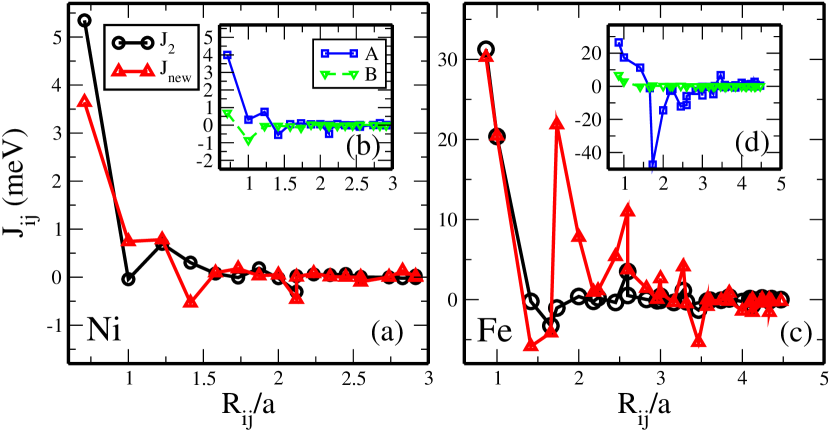
Figure 1: The MEI $J_{2}$ (circles) and $J_{\mathrm{new}}=J_{2}+\frac{J_{2}-J_{1}}{2}$ (triangles) calculated for bulk fcc Ni (a) and bcc Fe (c) with respect to the distance $R$ with $a$ being the lattice parameter. In the insets are plotted the terms $A$ and $B$ for Ni (b) and Fe (d). For reasons given below, the discrepancy between $J_{2}$ and $J_{\mathrm{new}}$ is much stronger for Fe compared to Ni.

In order to grasp some insight on the first term $J_{1}$ we propose to consider from the model Hamiltonian side terms beyond the Heisenberg model which are expected to be implicitly included in the DFT counterpart. The additional terms can be obtained from a perturbation expansion of the Hubbard modeltakahashi ; kurz . The first terms which have been added are the four-spin interactions, $H_{\mathrm{4-spin}}=-\sum_{\begin{subarray}{c}m\not=n\not=p\not=q\end{subarray}}K_{mnpq}[(\vec{e}_{m}\vec{e}_{n})(\vec{e}_{p}\vec{e}_{q})+(\vec{e}_{n}\vec{e}_{p})(\vec{e}_{q}\vec{e}_{m})+(\vec{e}_{m}\vec{e}_{p})(\vec{e}_{n}\vec{e}_{q})]/3$. Calculating the energy difference (eq. 3) due to the rotation of the atomic moments $i$ and $j$ leads to following further terms:

$$\Delta E_{i,j}^{\mathrm{4-spin}} = -K(1+\cos(\theta_{i})\cos(\theta_{j})-\cos(\theta_{i})-\cos(\theta_{j}))$$ (19)

$$-\frac{K}{3}(\sin(\theta_{i})\sin(\theta_{j})\cos(\phi_{i}-\phi_{j}))$$

with $K=\sum_{\begin{subarray}{c}p\not=q\\ p\not=i,j\\ q\not=i,j\end{subarray}}K_{ijpq}$.

Obviously, one notices that the four-spin interactions with the uncanted environment spins behave for the $ij$ pair like a bilinear term since only the moments $i$ and $j$ are canted. It is interesting to note that adding this term to the Heisenberg model brings an imbalance between the term proportional to the $\sin$ function and the one proportional to $\cos$. We conclude that this mechanism is behind the observed anisotropy in eq. 17. If we restrict ourself to the four-spin interactions only, the difference $J_{1}-J_{2}$ would be given by $2K/3$ that consequently would lead to a renormalization of $J_{ij}$ from $J_{2}$ to $J_{2}+\frac{J_{2}-J_{1}}{2}$ that we represented as $J_{\mathrm{new}}$ in Fig. 1. This final result is without any doubt subject to modification as soon as higher order terms are included in the model Hamiltonian. The extraction of the exact MEI is thus a rather difficult task. As mentioned previously, since the moment of Fe is higher than the one of Ni, the discrepancy between the renormalized $J_{ij}$ and $J_{2}$ is strongest for Fe (Fig. 1).

We exemplify the effect of such corrections by evaluating the new Curie temperatures ($T_{c}$) by Monte-Carlo simulations. The extracted temperatures are not expected to be correct but are meant as illustrative examples for the effect of renormalizing the MEI. A major result shown in Table 1 is the large increase of $T_{c}$ with the new values of the MEI for Ni, Co and Fe. The difference between the old and new temperature gets stronger when increasing the magnetic moment of the host. Surprisingly, similar behaviors have been obtained by Katsnelson and Lichtensteinkatsnelson when comparing the temperatures obtained using the renormalized method of Brunobruno with those of the old LKAG method. Obviously, the values obtained for Fe are too high and probably, one has to include higher order terms in the model Hamiltonian to lower $T_{c}$. The values obtained with only $J_{2}$ are probably sufficient for Fe due to a cancellation of errors that were described by Katsnelson and Lichtensteinkatsnelson .

Table 1: The Curie temperature (in K) for Ni, Fe and Co calculated with the LKAG formalism and with taking into account the 4-spin interactions.

$T_{c}$ (K)	Exp.	$J_{2}$	$J_{2}+\frac{(J_{2}-J_{1})}{2}$
Ni(fcc-LDA)	631	374	458
Co(fcc-GGA)	1388-1398	1520	1949
Fe(bcc-LDA)	1045	1086	2062
Fe(bcc-GGA)		1165	2791

By concluding we stress that the LKAG formula for $J_{ij}$ describes correctly the MEI for small canting angles $\theta$. In this case the spin-dependent $t$-matrices $\Delta t$ of Eq. 14 vary linearly in $\theta$, so that $\Delta E_{(i,j)}$ is proportional to $J_{ij}~{}\theta^{2}$ where $\theta$ is an effective canting angle. All higher order interactions like $K_{ijkl}$ between 4 or 6 slightly canted spins therefore scale as $\theta^{4}$ or $\theta^{6}$. As demonstrated, these $J_{ij}$ calculated by the LKAG formula include implicitly all multispin interactions of the canted $(i,j)$ moments with the uncanted environment atoms. It is for these reasons, that the calculated long-wave magnons and the spin stiffness constants agree very well with experiment. However, for larger transversal fluctuations of the moments the bilinear interaction $~{}J_{ij}$ is no longer sufficient, and higher order spin interactions like the four spin interaction and the biquadratic coupling become important and have to be included explicitly in calculating $T_{c}$ and related thermodynamic properties. Since the spin splitting and $\Delta t$ scale with the local moments $M$, these multispin interactions scale as $M^{4}$ or higher and are thus more important for systems with large moments. In the paper, we have demonstrated the importantce of four spin interactions in $T_{c}$-calculations for Fe, Co and Ni based on the LKAG formula for larger canting angles.

We are grateful to J. Kudrnovsky, I. Turek and S. Blügel for fruitful discussions. S. L. wishes to thank the Alexander von Humboldt Foundation for a Feodor Lynen Fellowship and D. L. Mills for discussions and hospitality.

References

- (1) Ph. Kurz, G. Bihlmayer, K. Hirai, and S. Blügel, Phys. Rev. Lett 86, 1106 (2001)
- (2) R. Drautz, M. Fahnle, Phys. Rev. B 69, 104404 (2004).
- (3) K. Park, M. R. Pederson, S. L. Richardson, N. Aliaga-Alcalde, G. Christou, Phys. Rev. B, 68, 020405(R) (2003)
- (4) M. Lezaic, Ph. Mavropoulos, S. Blügel, Appl. Phys. Lett, 90, 82504 (2007)
- (5) L. M. Sandratskii, R. Singer, E. Sasioglu, Phys. Rev. B, 76, 184406 (2007).
- (6) M. Bode, M. Heide, K. von Bergmann, P. Ferriani, S. Heinze, G. Bihlmayer, A. Kubetzka, O. Pietzsch, S. Blügel, R. Wiesendanger Nature 447, 190 (2007).
- (7) L. Udvardi, L. Szunyogh, Phys. Rev. Lett. 102, 207204 (2009).
- (8) M. Pajda, J. Kudrnovsky, I. Turek, V. Drchal, and P. Bruno, Phys. Rev. B 64, 174402 (2001); G. Bouzerar et al.Phys. Rev. B,68, 81203 (2003).
- (9) B. Belhadji, L. Bergqvist, R. Zeller, P. H. Dederichs, K. Sato and H. Katayama-Yoshida, J. Phys.: Condens. Matter. 19, 436227 (2007).
- (10) S. Lounis, Ph. Mavropoulos, P. H. Dederichs, and S. Blügel, Phys. Rev. B 72, 224437 (2005); S. Lounis, Ph. Mavropoulos, R. Zeller, P. H. Dederichs, and S. Blügel Phys. Rev. B 75, 174436 (2007);S. Lounis, M. Reif, Ph. Mavropoulos, L. Glaser, P. H. Dederichs, M. Martins, S. Blügel, W. Wurth, Eur. Phys. Lett. 81, 47004 (2008); S. Lounis, P. H. Dederichs, S. Blügel, Phys. Rev. Lett. 101, 107204 (2008).
- (11) A. Bergman, L. Nordström, A. B. Klautau, S. Frota-Pessoa, O. Eriksson, Phys. Rev. B 73, 174434 (2006); R. Robles, L. Nordstrom, Phys. Rev. B 74 094403 (2006).
- (12) O. Sipr, S. Bornemann, J. Minár, S. Polesya, V. Popescu, A. Simunek, and H. Ebert, J. Phys.: Condens. Matter 19, 096203 (2007); S. Mankovsky, S. Bornemann, J. Minar, S. Polesya, H. Ebert, J. B. Staunton, A. I. Lichtenstein, Phys. Rev. B 80 014422 (2009).
- (13) Ph. Mavropoulos, S. Lounis, S. Blügel, Phys. Stat. Sol. B 247, 1187 (2010); Ph. Mavropoulos, S. Lounis, R. Zeller, S. Blügel, Appl. Phys. A 82 103 (2006).
- (14) X. Wan, Q. Yin, S. Y. Savrasov, Phys. Rev. Lett. 97, 266403 (2006).
- (15) A. I. Liechtenstein, M. I. Katsnelson, V. P. Antropov, V. A. Gubanov, J. Magn. Magn. Mat 67, 65 (1987).
- (16) V. Heine, Solid State Phys. 35, 1 (1980).
- (17) A. Oswald, R. Zeller, P. J. Braspenning and P. H. Dederichs, J. Phys. F 15, 193 (1985).
- (18) P. Bruno, Phys. Rev. Lett. 90, 87205 (2003).
- (19) P. H. Dederichs et al. Phys. Rev. Lett. 53, 2512 (1984).
- (20) V. P. Antropov, J. Magn. Magn. Mat. 262 L192 (2003); V. P. Antropov, M. van Schilfgaarde, S. Brink and J. L. Xu, Journal of Appl. Phys. 99, 08F507 (2006).
- (21) M. I. Katsnelson, A. I. Lichtenstein, J. Phys.: Cond. Matter 16, 7439 (2004).
- (22) J. Callaway, C. S. Wang, D. G. Laurent, Phys. Rev. B 24, 6491 (1981).
- (23) S. Y. Savrasov, Phys. Rev. Lett., 81, 2570 (1998).
- (24) A. T. Costa, R. B. Muniz, D. L. Mills, Phys. Rev. B 69, 064413 (2004); ibid. 70, 054406 (2004); ibid. 73, 054426 (2006); A. T. Costa, R. B. Muniz, S. Lounis, A. B. Klautau, D. L. Mills, ibid. 82, 014428 (2010); A. T. Costa, R. B. Muniz, D. L. Mills, Phys. Rev. Lett. 94, 137203 (2005).
- (25) P. Buczek, A. Ernst, and L. M. Sandratskii, Phys. Rev. Lett. 105 097205 (2010).
- (26) E. Sasioglu, A. Schindlmayr, C. Friedrich, F. Freimuth, and S. Blügel, Phys. Rev. B 81, 054434 (2010).
- (27) J. B. Staunton, J. Poulter, B. Ginatempo, E. Bruno, and D. D. Johnson, Phys. Rev. Lett. 82, 3340 (1999).
- (28) S. Lounis, A. T. Costa, R. B. Muniz, D. L. Mills, Phys. Rev. Lett. 105, 187205 (2010); ibid., ArXiv:1010.1293 (2010); A. A. Khajetoorians, S. Lounis, B. Chilian, A. T. Costa, L. Zhou, D. L. Mills, R. Wiesendanger, and J. wiebe, ArXiv:1010.1284 (2010).
- (29) P. Lloyd, P. V. Smith, Advan. Phys. 21, 69 (1972).
- (30) B. Drittler, M. Weinert, R. Zeller, P. H. Dederichs, Phys. Rev. B 39, 930 (1989).
- (31) M. Takahashi, J. Phys. C 10, 1289 (1977).
- (32) N. Papanikolaou, R. Zeller, P. H. Dederichs, J. Phys.: Condens. Matter 14, 2799 (2002).
- (33) S. H. Vosko, L. Wilk, M. Nusair, J. Chem. Phys. 58, 1200 (1980).
- (34) J. P. Perdew, Y. Wang, Phys. Rev. B 45, 13244 (1992).