PUPT-2350

UT-Komaba/10-6

IFT-UAM/CSIC-10-51

Solutions from boundary condition changing operators
in open string field theory
Michael Kiermaier¹,  Yuji Okawa²  and  Pablo Soler^3
1 Princeton University
Princeton, NJ 08544, USA
mkiermai@princeton.edu ² Institute of Physics, University of Tokyo
Komaba, Meguro-ku, Tokyo 153-8902, Japan
okawa@hep1.c.u-tokyo.ac.jp ³ Instituto de Física Teórica UAM/CSIC
Universidad Autónoma de Madrid C-XVI
Cantoblanco, 28049 Madrid, Spain
pablo.soler@uam.es
Abstract

We construct analytic solutions of open string field theory using boundary condition changing (bcc) operators. We focus on bcc operators with vanishing conformal weight such as those for regular marginal deformations of the background. For any Fock space state $\phi$, the component string field $\langle\phi,\Psi\rangle$ of the solution $\Psi$ exhibits a remarkable factorization property: it is given by the matter three-point function of $\phi$ with a pair of bcc operators, multiplied by a universal function that only depends on the conformal weight of $\phi$. This universal function is given by a simple integral expression that can be computed once and for all. The three-point functions with bcc operators are thus the only needed physical input of the particular open string background described by the solution. We illustrate our solution with the example of the rolling tachyon profile, for which we prove convergence analytically. The form of our solution, which involves bcc operators instead of explicit insertions of the marginal operator, can be a natural starting point for the construction of analytic solutions for arbitrary backgrounds.

1 Introduction and summary

In the perturbative world-sheet formulation of string theory, consistent backgrounds are described by conformal field theories in two dimensions. In the nonperturbative formulation of string theory we are searching for, we expect that the requirement of conformal invariance in the world-sheet theory is reproduced from the classical equation of motion in the spacetime theory. String field theory is a candidate for such nonperturbative formulations, and we expect a correspondence between the space of conformal field theories and the space of classical solutions.

In the case of the open string, a consistent background is given by a choice of boundary conformal field theory (BCFT), and different open string backgrounds correspond to different conformal boundary conditions. The change of boundary conditions can be described by insertions of boundary condition changing (bcc) operators in the original BCFT. For example, the change of the boundary conditions on a segment of the world-sheet boundary from a point $a$ to a point $b$ can be described by inserting a pair of bcc operators $\sigma_{L}(a)$ and $\sigma_{R}(b)$. While bcc operators are generically not local, they transform as primary fields under conformal transformations.

A deformation of boundary conditions is called marginal when the new BCFT is continuously connected to the original BCFT by a one-parameter family of conformal boundary conditions. A primary field $V(t)$ of weight one in the matter sector generates an infinitesimal deformation of the BCFT, and conformal invariance is preserved to linear order in the deformation parameter which we denote by $\lambda$. When operator products of the marginal operator $V(t)$ are regular, finite deformations also preserve conformal invariance and thus the operator $V(t)$ generates a family of boundary conditions parameterized by $\lambda$. In this case, the change of boundary conditions on a segment $[\,a,b\,]$ can be implemented by

$$\sigma_{L}(a)\,\sigma_{R}(b)~{}=~{}\exp\,\biggl{[}\,\lambda\int_{a}^{b}dt\,V(t)\,\biggr{]}\,.$$ (1.1)

The bcc operators associated with such regular marginal deformations have vanishing conformal weights and satisfy

$$\lim_{\epsilon\to 0}\sigma_{L}(0)\,\sigma_{R}(\epsilon)=1\,,\qquad\lim_{\epsilon\to 0}\sigma_{L}(a)\,\sigma_{R}(b)\,\sigma_{L}(b+\epsilon)\,\sigma_{R}(c)=\sigma_{L}(a)\,\sigma_{R}(c)\,.$$ (1.2)

The correspondence between conformal invariance in the world-sheet theory and the equation of motion in the spacetime theory can therefore be restated in the case of the open string as a correspondence between a pair of bcc operators and a solution to open string field theory (OSFT). The equation of motion for open bosonic string field theory [1] is given by

$$Q\Psi+\Psi\ast\Psi\,=\,0\,,$$ (1.3)

where $\Psi$ is an open string field of ghost number one, $Q$ is the BRST operator, and the symbol $\ast$ denotes multiplication of string fields using Witten’s star product. Since the construction of an analytic solution to (1.3) by Schnabl [2], an impressive amount of analytic results for string field theory have been obtained [3, 4, 5, 6, 7, 8, 9, 10, 11, 12, 13, 14, 15, 16, 17, 18, 19, 20, 21, 22, 23, 24, 25, 26, 27, 28, 29, 30, 31, 32, 33, 34, 35, 36, 37, 38, 39, 40, 41, 42, 43, 44, 45, 46, 47, 48, 49, 50, 51, 52, 53, 54, 55, 56, 57, 58]. These results partially illuminate the connection between the BCFT and OSFT descriptions of open string backgrounds. In particular, inspired by Ellwood’s interpretation [31] of the gauge-invariant observable [59, 60] as the closed-string tadpole, an OSFT construction of the BCFT boundary state associated with known analytic solutions was presented in [40].

The other direction of the correspondence, namely, the construction of OSFT solutions associated with a given BCFT remains illusive. Ideally, we would like to find a systematic construction of an OSFT solution from any given pair of bcc operators $\sigma_{L}$ and $\sigma_{R}$. Partial progress in this direction was achieved in [22], where analytic solutions for general marginal deformations were constructed from the bcc operators (1.1). Unfortunately, the solution in [22] does not seem to be the most promising starting point to construct analytic solutions for more general open string backgrounds. First of all, it was crucial for the construction in [22] to expand the nonlocal operator $\sigma_{L}(a)\sigma_{R}(b)$ in powers of the deformation parameter $\lambda$. For bcc operators that describe generic open string backgrounds, no such expansion parameter is available and there are no straightforward ways to generalize the construction. The second problem is more technical in nature. The solution in [22] is constructed from wedge-based states of integer width. In particular, the shortest wedge-based state appearing in the solution has nonvanishing width. As the wedge width is additive under star multiplication, the operators inserted on this shortest wedge state must be BRST-closed to satisfy the equation of motion (1.3). For generic open string backgrounds, however, there are no natural candidates for such operator insertions.

There is another unsatisfactory feature shared by all known analytic solutions for marginal deformations. When we calculate a coefficient of the solution $\Psi$ given by the BPZ inner product $\langle\phi,\Psi\rangle$ for a state $\phi$ in the Fock space, one needs explicit knowledge of all $n$-point matter correlation functions

$$\Bigl{\langle}\phi_{m}(0)V(t_{1})V(t_{2})\ldots V(t_{n})\Bigr{\rangle}_{\rm UHP,\,matter}\,,$$ (1.4)

where $\phi_{m}$ is the matter part of $\phi$ and UHP stands for upper half-plane. These correlators are necessary for $\langle\phi,\Psi\rangle$ at order $\lambda^{n}$ and are integrated over $t_{i}$ in a particular way. Therefore the coefficient $\langle\phi,\Psi\rangle$ has to be calculated from scratch for each choice of the matter operator $\phi_{m}$ and the marginal operator $V$. All information about a change in boundary conditions by $\sigma_{L}(a)\sigma_{R}(b)$, however, should in principle be captured entirely by the matter three-point functions

$$C_{\phi}=\bigl{\langle}\phi_{m}(0)\sigma_{L}(1)\sigma_{R}(\infty)\bigr{\rangle}_{\rm UHP,\,matter}\,\,.$$ (1.5)

This aspect is obscured in all previously known analytic solutions for marginal deformations.

In this paper, we present solutions for regular marginal deformations without any of the unsatisfactory features mentioned above. The solution consists of wedge-based states, and its operator insertions depend on the matter sector only through bcc operators and their BRST transformations. The solution is given by

$$\begin{split}\Psi&=-\frac{1}{\sqrt{1-K}}\,(Q\sigma_{L})\,\frac{1}{1-K}\sigma_{R}\,(1-K)Bc\frac{1}{\sqrt{1-K}}\,,\end{split}$$ (1.6)

where $K$, $B$, $c$, $\sigma_{L}$, and $\sigma_{R}$ are states based on the wedge state of zero width with a line integral of the energy-momentum tensor and the $b$ ghost for $K$ and $B$, respectively, and with a local insertion of the $c$ ghost, $\sigma_{L}(t)$, and $\sigma_{R}(t)$ for $c$, $\sigma_{L}$, and $\sigma_{R}$, respectively. The state $K$ is the BRST transformation of $B$, and the wedge state $W_{\alpha}$ of width $\alpha$ is generated from $K$ as $W_{\alpha}=e^{\alpha K}$.

The solution $\Psi$ in (1.6) is a special case of a class of analytic solutions for regular marginal deformations constructed by Erler [15], just as the “simple” analytic solution for tachyon condensation of [48] is a special case of a class of solutions in [3]. It is interesting to note that exactly the same replacement $e^{K}\!\to 1/(1-K)$, which was used in [48] to transform the Schnabl-gauge solution, also appears in our analysis. Up to scaling of $K$, it is the unique replacement that gives a solution based on bcc operators. Using Laplace transforms of $1/(1-K)$ and $1/\sqrt{1-K}$ , we can express the solution (1.6) in terms of wedge-based states:

$$\Psi=-\int_{0}^{\infty}dr\int_{0}^{\infty}ds\int_{0}^{\infty}dt\,\frac{e^{-r-s-t}}{\pi\sqrt{rt}}\ e^{rK}(Q\sigma_{L})\,e^{sK}\sigma_{R}\,(1-K)Bc\,e^{tK}\,.$$ (1.7)

Note that no expansion of the bcc operators in $\lambda$ is necessary to define the solution. Furthermore, the solution takes the form of an integral over wedge-based states of width in the entire range $[\,0,\infty)$ , and we thus expect it to be a natural starting point for the construction of analytic solutions for more general backgrounds.

The calculation of coefficients $\langle\phi,\Psi\rangle$ for this solution reduces to a simple evaluation of the three-point function $C_{\phi}$ in (1.5). For example, consider any operator $\phi$ of the form

$$\phi=-c\partial c\,\phi_{m}\,,$$ (1.8)

where $\phi_{m}$ is a matter primary field of weight $h\geq 1$. The coefficient $\langle\phi,\Psi\rangle$ in this case is simply given by

$$\bigl{\langle}\,\phi\,,\,\Psi\,\bigr{\rangle}~{}=~{}C_{\phi}\,g(h)\,,$$ (1.9)

where $g(h)$ is a universal function of the weight $h$ of $\phi_{m}$, but otherwise it is independent of the particular choice of $\phi_{m}$ or the marginal operator $V$. The explicit form of the function $g(h)$ is given by

$$\begin{split}g(h)~{}&=~{}\frac{h(h-1)}{2\pi}\,\int_{\frac{1}{2}}^{\infty}dx\int_{0}^{\infty}ds\int_{\frac{1}{2}}^{\infty}dy\,\frac{e^{1-x-s-y}}{\sin^{2}\theta_{s}\sqrt{(x-\tfrac{1}{2})(y-\tfrac{1}{2})}}\,\biggl{|}\,\frac{2\sin\theta_{s}}{L\sin\theta_{x}\sin\theta_{y}}\,\biggr{|}^{h}\\ &\hskip 136.5733pt\times\Bigl{[}\,\theta_{y}\,\sin^{2}\theta_{x}+\theta_{x}\,\sin^{2}\theta_{y}-\sin{\theta_{x}}\,\sin{\theta_{s}}\,\sin{\theta_{y}}\,\Bigr{]}\qquad\text{ for }~{}h>1\,,\end{split}$$ (1.10)

where $L=x+s+y$, and $\theta$ with a subscript is defined by $\theta_{\ell}=\frac{\ell}{L}\,\pi$. At $h=1$ and for large $h$, the function $g(h)$ takes the form

$$g(1)\,=\,1\,,\qquad~{}~{}g(h)\,\sim\,\biggl{(}\frac{8}{\pi}\biggr{)}^{h}~{}~{}\text{ for }~{}h\gg 1\,.$$ (1.11)

This exact result for the large-$h$ behavior of $g(h)$ will allow us to prove the convergence of the tachyon profile of the rolling tachyon solution. A plot of $g(h)$ is presented in figure 1 of section 3.

This paper is organized as follows. In section 2 we derive the solution (1.6) as a special case of a class of analytic solutions for regular marginal deformations constructed by Erler [15]. In section 3 we establish the universal behavior (1.9) of coefficients $\langle\phi,\Psi\rangle$ and study the asymptotic behavior of the function $g(h)$. As an application, the results for $g(h)$ are then used in section 4 to extract the tachyon profile from the rolling tachyon solution.

2 Derivation of the solution

Analytic solutions for marginal deformations were first constructed in [13, 14] when operator products of the marginal operator $V(t)$ are regular. The solutions are given as a perturbative expansion in the deformation parameter $\lambda$:

$$\Psi=\sum_{n=1}^{\infty}\lambda^{n}\Psi^{(n)}\,.$$ (2.1)

Expressed as a conformal field theory (CFT) correlator, $\Psi^{(n)}$ in Schnabl gauge [13, 14] is given by

$$\begin{split}\langle\,\phi,\Psi^{(n)}\,\rangle&=\int_{0}^{1}\hskip-3.0ptdt_{1}\int_{0}^{1}\hskip-3.0ptdt_{2}\ldots\int_{0}^{1}\hskip-3.0ptdt_{n-1}\,\langle\,f\!\circ\!\phi(0)\,cV(1)\,{\cal B}\,cV(1+t_{1})\,{\cal B}\,cV(1+t_{1}+t_{2})\,\ldots\\ &\qquad\qquad\qquad\qquad\qquad\qquad\,{}\times{\cal B}\,cV(1+t_{1}+t_{2}+\ldots+t_{n-1})\,\rangle_{{\cal W}_{1+t_{1}+t_{2}+\ldots+t_{n-1}}}\,.\end{split}$$ (2.2)

Here and in what follows we denote a generic state in the Fock space by $\phi$ and its corresponding operator in the state-operator mapping by $\phi(\xi)$. We denote the conformal transformation of $\phi(\xi)$ under the map $f(\xi)$ by $f\circ\phi(\xi)$, where

$$f(\xi)=\frac{2}{\pi}\,\arctan\xi\,.$$ (2.3)

The correlation function is evaluated on the wedge surface ${\cal W}_{\alpha}$ with $\alpha\geq 0$, which is the semi-infinite strip on the upper half-plane of $z$ between the vertical lines $\Re(z)=-\frac{1}{2}$ and $\Re(z)=\frac{1}{2}+\alpha$ with these lines identified by translation. The operator ${\cal B}$ is a line integral of the $b$ ghost defined by

$${\cal B}=\int_{i\infty}^{-i\infty}\frac{dz}{2\pi i}\,b(z)\,,$$ (2.4)

where we used the doubling trick. Its BRST transformation is given by

$${\cal K}=\int_{i\infty}^{-i\infty}\frac{dz}{2\pi i}\,\oint\frac{dw}{2\pi i}\,j_{B}(w)\,b(z)=\int_{i\infty}^{-i\infty}\frac{dz}{2\pi i}\,T(z)\,,$$ (2.5)

where $j_{B}$ is the BRST current, $T$ is the energy-momentum tensor, and the contour of the integral over $w$ encircles $z$ counterclockwise. The line integral ${\cal K}$ of the energy-momentum tensor is the generator of infinitesimal changes in the width of the wedge state $W_{\alpha}$ defined by

$$\langle\,\phi,W_{\alpha}\,\rangle=\langle\,f\!\circ\!\phi(0)\rangle_{{\cal W}_{\alpha}}\,.$$ (2.6)

Indeed, we have

$$\langle\,\phi,\partial_{\alpha}W_{\alpha}\,\rangle=\langle\,f\!\circ\!\phi(0)\,{\cal K}\,\rangle_{{\cal W}_{\alpha}}\,.$$ (2.7)

The solution (2.2) can also be expressed in an algebraic language without referring to explicit CFT correlators. We denote by $K$ the string field that generates the wedge states through the relation

$$W_{\alpha}=e^{\alpha K}\,.$$ (2.8)

We can think of $K$ as a wedge state of zero width with an insertion of ${\cal K}$:

$$\langle\,\phi,K\,\rangle=\langle\,f\!\circ\!\phi(0)\,{\cal K}\,\rangle_{{\cal W}_{0}}\,.$$ (2.9)

Note that the identity (2.7) is manifest in this algebraic language:

$$\partial_{\alpha}e^{\alpha K}=e^{\alpha K}K\,.$$ (2.10)

We denote analogous wedge-based states of zero width with insertions of ${\cal B}$, $c(\frac{1}{2})$, and $V(\frac{1}{2})$ on the wedge surface ${\cal W}_{0}$ by $B$, $c$, and $V$, respectively. These states satisfy the following relations:

$$\begin{split}[K,B]=0\,,\qquad[B,V]=0\,,\qquad[c,V]=0\,,\qquad c^{2}=0\,,\qquad B^{2}=0\,,\qquad\{B,c\}=1\,.\end{split}$$ (2.11)

The BRST transformation $Q$ acts on these states in the following way:

$$QB=K\,,\qquad QK=0\,,\qquad Qc=cKc\,,\qquad QV=[K,cV]\,.$$ (2.12)

It follows that $Q\,(cV)=0$, which expresses the marginality of the operator $V$.

In this algebraic language, the solution (2.2) takes the form

$$\Psi^{(n)}=e^{K/2}cV\Bigl{(}\int_{0}^{1}dt\,Be^{tK}cV\Bigr{)}^{n-1}e^{K/2}=e^{K/2}cV\Bigl{(}B\frac{e^{K}-1}{K}cV\Bigr{)}^{n-1}e^{K/2}\,.$$ (2.13)

The perturbative series in $\lambda$ that defines $\Psi$ in (2.1) can then be summed to obtain

$$\Psi=\lambda e^{K/2}cV\Bigl{(}1-\lambda B\frac{e^{K}-1}{K}cV\Bigr{)}^{-1}e^{K/2}\,.$$ (2.14)

In [15], Erler showed that gauge-equivalent solutions can be obtained if one replaces $e^{K/2}$ appearing in (2.14) by a general function $f(K)$:

$$\Psi=f(K)\,\lambda\,cV\,\biggl{[}\,1-B\,\frac{f(K)^{2}-1}{K}\,\lambda\,cV\,\biggr{]}^{-1}f(K)\,.$$ (2.15)

To avoid the wedge state $W_{\alpha}=e^{\alpha K}$ with negative $\alpha$, we require $f(K)$ to take the following form:

$$f(K)=\int_{0}^{\infty}dt\,\tilde{f}(t)\,e^{tK}\,.$$ (2.16)

We are looking for a choice of $f(K)$ that allows us to express $\Psi$ in terms of bcc operators. Consider the wedge state with a boundary condition modified by a marginal deformation generated by the operator $V(t)$. An insertion of

$$\exp\,\biggl{[}\,\lambda\int_{a}^{b}dt\,V(t)\,\biggr{]}=1+\lambda\int_{a}^{b}dt_{1}\,V(t_{1})+\lambda^{2}\int_{a}^{b}dt_{1}\int_{t_{1}}^{b}dt_{2}\,V(t_{1})\,V(t_{2})\,+\ldots$$ (2.17)

corresponds to changing the wedge state $e^{\alpha K}$ with $\alpha=b-a$ to $U_{\alpha}$ given by

$$U_{\alpha}=e^{\alpha K}+\lambda\int_{0}^{\alpha}dt_{1}\,e^{t_{1}K}\,V\,e^{(\alpha-t_{1})K}+\lambda^{2}\int_{0}^{\alpha}dt_{1}\int_{t_{1}}^{\alpha}dt_{2}\,e^{t_{1}K}\,V\,e^{(t_{2}-t_{1})K}\,V\,e^{(\alpha-t_{2})K}+\ldots\,.$$ (2.18)

When $\alpha$ is small, $U_{\alpha}$ reduces to

$$U_{\alpha}=1+\alpha\,(K+\lambda V)+{\cal O}(\alpha^{2})\,.$$ (2.19)

We can also show that $U_{\alpha+\beta}$ factorizes as

$$U_{\alpha+\beta}~{}=~{}U_{\alpha}\,U_{\beta}\,,$$ (2.20)

which is obvious from the structure of $U_{\alpha}$ similar to that of the path-ordered exponential. From these two properties, we conclude that

$$U_{\alpha}=e^{\alpha(K+\lambda\,V)}\,.$$ (2.21)

Therefore, the wedge state with the modified boundary condition is given by $e^{\alpha(K+\lambda\,V)}$. In the language of bcc operators, this can be stated as follows:

$$\ldots\,e^{\alpha(K+\lambda\,V)}\,\ldots~{}=~{}\ldots\,\sigma_{L}\,e^{\alpha K}\,\sigma_{R}\,\ldots\,,$$ (2.22)

where the dots $\ldots$ represent arbitrary wedge-based states with the boundary conditions of the undeformed BCFT. Let us next consider the BRST transformation of the state $e^{\alpha(K+\lambda\,V)}$. We use the formula

$$\delta\,e^{\alpha M}=\int_{0}^{\alpha}dt\,e^{tM}\,\delta M\,e^{(\alpha-t)M}$$ (2.23)

for any derivation $\delta(M_{1}M_{2})=(\delta M_{1})\,M_{2}+M_{1}\,(\delta M_{2})$ with respect to the multiplication under consideration. For star products of Grassmann-even states, the BRST transformation $Q(M_{1}M_{2})=(QM_{1})\,M_{2}+M_{1}\,(QM_{2})$ and the commutator $[\,N,\,M_{1}M_{2}\,]=[\,N,\,M_{1}\,]\,M_{2}+M_{1}\,[\,N,\,M_{2}\,]$ are such derivations. Since

$$Q\,(K+\lambda V)=[\,K+\lambda V,\,\lambda\,cV\,]\,,$$ (2.24)

which follows from (2.12), we find that

$$\begin{split}Q\,e^{\alpha(K+\lambda\,V)}&=\int_{0}^{\alpha}dt\,e^{t(K+\lambda\,V)}\,Q\,(K+\lambda V)\,e^{(\alpha-t)(K+\lambda\,V)}\\ &=\int_{0}^{\alpha}dt\,e^{t(K+\lambda\,V)}\,[\,K+\lambda V,\,\lambda\,cV\,]\,e^{(\alpha-t)(K+\lambda\,V)}\\[2.15277pt] &=e^{\alpha(K+\lambda\,V)}\,\lambda\,cV-\lambda\,cV\,e^{\alpha(K+\lambda\,V)}\,.\end{split}$$ (2.25)

In the language of bcc operators, we can write

$$\begin{split}\ldots\,e^{\alpha(K+\lambda\,V)}(\lambda\,cV)\,\ldots~{}&=~{}\ldots\,\sigma_{L}\,e^{\alpha K}\,(Q\,\sigma_{R})\,\ldots\,,\\ \ldots\,(-\lambda\,cV)\,e^{\alpha(K+\lambda\,V)}\,\ldots~{}&=~{}\ldots\,(Q\,\sigma_{L})\,e^{\alpha K}\,\sigma_{R}\,\ldots\,.\end{split}$$ (2.26)

Our goal is to find a choice of $f(K)$ such that the solution $\Psi$ can be written in terms of $\sigma_{L}$ and $\sigma_{R}$ and their BRST transformations without using $V$ explicitly. This is achieved if $\lambda V$ only appears in the solution through the combination $h(K+\lambda V)$, $h(K+\lambda V)(\lambda cV)$, or $(\lambda cV)h(K+\lambda V)$ with arbitrary functions $h(x)$ in the following form:

$$h(x)=\int_{0}^{\infty}d\alpha\,\tilde{h}(\alpha)\,e^{\alpha x}\,.$$ (2.27)

This ensures that $h(K+\lambda V)$ has support on wedge states of nonnegative width. Indeed,

$$h(K+\lambda V)=\int_{0}^{\infty}d\alpha\,\tilde{h}(\alpha)\,e^{\alpha(K+\lambda V)}\,.$$ (2.28)

It then follows from (2.22) and (2.26) that

$$\boxed{\begin{aligned} \phantom{\Bigl{(}}\ldots\,h(K+\lambda\,V)\,\ldots~{}&=~{}\ldots\,\sigma_{L}\,h(K)\,\sigma_{R}\,\ldots\,,\\ \ldots\,h(K+\lambda\,V)(\lambda\,cV)\,\ldots~{}&=~{}\ldots\,\sigma_{L}\,h(K)\,(Q\,\sigma_{R})\,\ldots\,,\\ ~{}~{}\ldots\,(\!{}-\!\lambda\,cV)\,h(K+\lambda\,V)\,\ldots~{}&=~{}\ldots\,(Q\,\sigma_{L})\,h(K)\,\sigma_{R}\,\ldots\,.\phantom{\Bigl{(}}~{}\end{aligned}}$$ (2.29)

To find a choice of $f(K)$ that brings the solution (2.15) into this form, it is convenient to first transform $\Psi$ slightly. As shown in appendix A.1, the solution can be written as

$$\begin{split}\Psi&=f(K)\,\lambda\,cV\,\biggl{[}\,1-\frac{f(K)^{2}-1}{K}\,\lambda\,V\,\biggr{]}^{-1}Bc\,f(K)\,.\end{split}$$ (2.30)

To obtain an expression for $\Psi$ in terms of (a finite number of) bcc operators, we choose

$$f(K)=\frac{1}{\sqrt{1-K}}\,.$$ (2.31)

The derivation of this is presented in appendix A.2. With this choice, we have

$$\boxed{\begin{aligned} \phantom{\Biggl{(}}\Psi&=~{}\frac{1}{\sqrt{1-K}}\,\lambda\,cV\,\frac{1}{1-K-\lambda\,V}(1-K)Bc\frac{1}{\sqrt{1-K}}\\[-4.30554pt] &=-\frac{1}{\sqrt{1-K}}\,(Q\sigma_{L})\,\frac{1}{1-K}\sigma_{R}\,(1-K)Bc\frac{1}{\sqrt{1-K}}\,,\phantom{\Biggl{(}}\end{aligned}~{}}$$ (2.32)

where we used the identity

$$\biggl{[}\,1-\frac{1}{1-K}\,\lambda\,V\,\biggr{]}^{-1}=\frac{1}{1-K-\lambda\,V}(1-K)\,.$$ (2.33)

It is easy to expand this solution as a superposition of wedge-based states. Using

$$\frac{1}{1-K}=\int_{0}^{\infty}ds\,e^{-s}e^{sK}\,,\qquad\frac{1}{\sqrt{1-K}}=\int_{0}^{\infty}ds\,\frac{e^{-s}}{\sqrt{\pi s}}\,e^{sK}\,,$$ (2.34)

we obtain

$$\Psi=-\int_{0}^{\infty}dr\int_{0}^{\infty}ds\int_{0}^{\infty}dt\frac{e^{-r-s-t}}{\pi\sqrt{rt}}\,e^{rK}\,(Q\sigma_{L})\,e^{sK}\sigma_{R}\,(1-K)Bc\,e^{tK}\,.$$ (2.35)

Let us also present the solution $\Psi$ in the CFT language. Recalling that the line integrals associated with $K$ and $B$ are denoted by ${\cal K}$ and ${\cal B}$, respectively, we have

$$\bigl{\langle}\phi\,,\,\Psi\bigr{\rangle}=-\!\!\int_{0}^{\infty}\!\!\!\!\!dr\!\int_{0}^{\infty}\!\!\!\!\!\!ds\!\int_{0}^{\infty}\!\!\!\!\!\!dt\,\frac{e^{-r-s-t}}{\pi\sqrt{rt}}\Bigl{\langle}f\circ\phi(0)~{}Q\sigma_{L}\bigl{(}\tfrac{1}{2}+r\bigr{)}\,\sigma_{R}\bigl{(}\tfrac{1}{2}+r+s\bigr{)}\,(1-{\cal K})\,{\cal B}\,c\bigl{(}\tfrac{1}{2}+r+s\bigr{)}\!\Bigr{\rangle}_{{\cal W}_{r+s+t}}\!\!\!\!.\,\,\,$$ (2.36)

The solution $\Psi$ satisfies the reality condition on the string field [63], but it is not manifest in (2.32). This can be seen as follows:

$$\begin{split}\Psi&=~{}\frac{1}{\sqrt{1-K}}\,\lambda\,cV\,\frac{1}{1-K-\lambda\,V}\,\bigl{[}\,(1-K-\lambda\,V)+\lambda\,V\,\bigr{]}\,Bc\,\frac{1}{\sqrt{1-K}}\\ &=~{}\frac{1}{\sqrt{1-K}}\,\lambda\,cV\,\frac{1}{\sqrt{1-K}}+\frac{1}{\sqrt{1-K}}\,\lambda\,cV\,\frac{B}{1-K-\lambda\,V}\,\lambda\,cV\,\frac{1}{\sqrt{1-K}}\,.\end{split}$$ (2.37)

This form is manifestly symmetric when we reverse the order of multiplication of string fields and thus satisfies the reality condition of [63], which guarantees that the string field theory action is real. In terms of bcc operators, this can be written in the following form:

$$\boxed{~{}~{}\Psi\,=\,-\frac{1}{\sqrt{1-K}}\,(Q\sigma_{L})\,\sigma_{R}\frac{1}{\sqrt{1-K}}\,\,-\,\,\frac{1}{\sqrt{1-K}}\,(Q\sigma_{L})\,\frac{B}{1-K}\,(Q\sigma_{R})\,\frac{1}{\sqrt{1-K}}\,.~{}~{}}$$ (2.38)

Although we arrived at this form from an expression that contained the marginal parameter $\lambda$ and operator $V$ explicitly, it is now written only in terms of $K$, $B$, $\sigma_{L}$, and $\sigma_{R}$. This is a solution to the equation of motion for any choice of bcc operators $\sigma_{L}$, $\sigma_{R}$ in the matter sector that satisfy the operator products (1.2), with $K$ and $B$ defined around (2.9).

More generally, (2.38) satisfies the equation of motion for any choice of three states $B$, $\sigma_{L}$, and $\sigma_{R}$ satisfying the relations

$$B^{2}=0\,,\qquad[\,B,\sigma_{L}\,]=0\,,\qquad[\,B,\sigma_{R}\,]=0\,,\qquad\sigma_{L}\,\sigma_{R}=1\,,\qquad\sigma_{R}\,\sigma_{L}=1\,,$$ (2.39)

and $K=QB$ serving as a definition of $K$. By considering the BRST transformation of each of the relations in (2.39), we find

$$\begin{split}&[\,K,B\,]=0\,,\quad\{\,B,Q\sigma_{L}\,\}=[\,K,\sigma_{L}\,]={}-[\,1-K,\sigma_{L}\,]\,,\quad\{\,B,Q\sigma_{R}\,\}=[\,K,\sigma_{R}\,]={}-[\,1-K,\sigma_{R}\,]\,,\\[4.30554pt] &(Q\sigma_{L})\,\sigma_{R}+\sigma_{L}\,(Q\sigma_{R})=0\,,\qquad(Q\sigma_{R})\,\sigma_{L}+\sigma_{R}\,(Q\sigma_{L})=0\,.\end{split}$$ (2.40)

We can verify that the solution (2.38) satisfies the equation of motion only from (2.39) and (2.40), and no explicit reference to $\lambda$ and $V$ or to the surface state definitions of $K$ and $B$ is necessary. Incidentally, we do not need to assume that $(Q\sigma_{L})\,(Q\sigma_{R})$ vanishes, while it does for regular marginal deformations we started with.

3 Universal coefficients

In the CFT language, the solution $\Psi$ is specified by giving $\langle\phi,\Psi\rangle$ for an arbitrary state $\phi$ in the Fock space. We can choose a basis of states in the Fock space such that the matter and ghost sectors are factorized. In this section we demonstrate that, when $\phi$ is in the factorized basis and its matter part is a primary field,  the inner product $\langle\phi,\Psi\rangle$ is given by a product of a universal $V$-independent factor and a simple three-point function of the matter part of $\phi$ with the bcc operators $\sigma_{L}$ and $\sigma_{R}$.

Since we are considering bcc operators with vanishing conformal weight, their BRST transformations are given by $Q\sigma_{L}=c\partial\sigma_{L}$ and $Q\sigma_{R}=c\partial\sigma_{R}$. The solution $\Psi$ in the form (2.38) can then be written as

$$\Psi\,=\,-\frac{1}{\sqrt{1-K}}\,(c\partial\sigma_{L})\,\sigma_{R}\frac{1}{\sqrt{1-K}}\,\,-\,\,\frac{1}{\sqrt{1-K}}\,(c\partial\sigma_{L})\,\frac{B}{1-K}\,(c\partial\sigma_{R})\,\frac{1}{\sqrt{1-K}}\,.$$ (3.1)

Let us calculate the inner product $\langle\phi,\Psi\rangle$ for $\phi=-c\partial c\,\phi_{m}$, where $\phi_{m}$ is a matter primary field of weight $h$. The first term in (3.1) is a superposition of wedge states with a single insertion of $(c\partial\sigma_{L})\,\sigma_{R}=-\lambda cV$, and its inner product with $\phi$ thus vanishes unless $h=1$. We postpone the special case $h=1$, and first consider the case $h>1$. It is then sufficient to evaluate the second term. We have

$$\langle\phi,\Psi\rangle\,=\,-\int_{\frac{1}{2}}^{\infty}dx\int_{0}^{\infty}ds\int_{\frac{1}{2}}^{\infty}dy\,\frac{e^{1-x-s-y}}{\pi\sqrt{(x-\tfrac{1}{2})(y-\tfrac{1}{2})}}\,\Bigl{\langle}\,f\!\circ\!\phi(0)\,c\partial\sigma_{L}(x)\,{\cal B}\,c\partial\sigma_{R}(x+s)\,\Bigr{\rangle}_{{\cal W}_{L-1}}\,,$$ (3.2)

where we have defined

$$L=x+s+y\,.$$ (3.3)

The correlator in (3.2) can be written in a matter-ghost factorized form as

$$\begin{split}&\langle\,f\!\circ\!\phi(0)\,c\partial\sigma_{L}(x)\,{\cal B}\,c\partial\sigma_{R}(x+s)\,\rangle_{{\cal W}_{L-1}}\\ &=-\frac{\pi}{2}\,\langle\,c\partial c(0)\,c(x)\,{\cal B}\,c(x+s)\,\rangle_{{\cal W}_{L-1},\,{\rm ghost}}\,\times\,\partial_{a}\partial_{b}\,\bigr{\langle}\!\!\langle\,f\!\circ\!\phi_{m}(0)\,\sigma_{L}(a)\,\sigma_{R}(b)\,\rangle\!\!\bigr{\rangle}_{{\cal W}_{L-1}}\biggr{|}_{a=x,\,b=x+s}\,,\end{split}$$ (3.4)

where we use $\bigr{\langle}\!\!\langle\ldots\rangle\!\!\bigr{\rangle}$ to denote matter correlators $\langle\ldots\rangle_{\rm matter}$. Since $\phi_{m}$, $\sigma_{L}$, and $\sigma_{R}$ are primary fields of weight $h$, $0$, and $0$, respectively, we find

$$\begin{split}\bigr{\langle}\!\!\langle\,f\!\circ\!\phi_{m}(0)\,\sigma_{L}(a)\,\sigma_{R}(b)\,\rangle\!\!\bigr{\rangle}_{{\cal W}_{L-1}}&\,=\,\Bigl{(}\frac{2}{L}\Bigr{)}^{h}\bigr{\langle}\!\!\langle\,f\!\circ\!\phi_{m}(0)\,\sigma_{L}\Bigl{(}\frac{2a}{L}\Bigr{)}\,\sigma_{R}\Bigl{(}\frac{2b}{L}\Bigr{)}\,\rangle\!\!\bigr{\rangle}_{{\cal W}_{1}}\\[2.15277pt] &\,=\,\Bigl{(}\frac{2}{L}\Bigr{)}^{h}\bigr{\langle}\!\!\langle\,\phi_{m}(0)\,\sigma_{L}\bigl{(}\tan\theta_{a}\bigr{)}\,\sigma_{R}\bigl{(}\tan\theta_{b}\bigr{)}\,\rangle\!\!\bigr{\rangle}_{{\rm UHP}}\\[2.15277pt] &\,=\,C_{\phi}\,\Bigl{|}\,\frac{2\,\sin\theta_{b-a}}{L\sin\theta_{a}\sin\theta_{b}}\Bigr{|}^{h}\,,\end{split}$$ (3.5)

where $\theta$ with a subscript is defined by

$$\theta_{\ell}=\frac{\ell}{L}\,\pi\,,$$ (3.6)

and $C_{\phi}$ is a constant independent of $a$, $b$, and $L$. It is related to the coefficient of the matter three-point function of $\phi$, $\sigma_{L}$ and $\sigma_{R}$ as follows:

$$\bigr{\langle}\!\!\langle\,\phi_{m}(z_{1})\,\sigma_{L}(z_{2})\,\sigma_{R}(z_{3})\,\rangle\!\!\bigr{\rangle}_{{\rm UHP}}~{}=~{}C_{\phi}\,\biggl{|}\frac{z_{2}-z_{3}}{(z_{1}-z_{2})(z_{1}-z_{3})}\biggr{|}^{h}\,.$$ (3.7)

In other words, $C_{\phi}$ is the matter three-point function with operators $\phi_{m}$, $\sigma_{L}$, and $\sigma_{R}$ inserted at $0$, $1$, and $\infty$, respectively:

$$C_{\phi}={}\bigr{\langle}\!\!\langle\,\phi_{m}(0)\,\sigma_{L}(1)\,\sigma_{R}(\infty)\,\rangle\!\!\bigr{\rangle}_{{\rm UHP}}\,.$$ (3.8)

For the matter correlator in (3.4), we then have

$$\begin{split}&\partial_{a}\partial_{b}\,\bigr{\langle}\!\!\langle\,f\!\circ\!\phi_{m}(0)\,\sigma_{L}(a)\,\sigma_{R}(b)\,\rangle\!\!\bigr{\rangle}_{{\cal W}_{L-1}}\biggr{|}_{a=x,\,b=x+s}\!=\,{}-C_{\phi}\,\frac{\pi^{2}h(h-1)}{L^{2}\sin^{2}\theta_{s}}\,\biggl{|}\,\frac{2\sin\theta_{s}}{L\sin\theta_{x}\sin\theta_{y}}\,\biggr{|}^{h}\,.\end{split}$$ (3.9)

The ghost sector correlator takes the form

$$\begin{split}\langle\,c\partial c(0)\,c(x)\,{\cal B}\,c(x+s)\,\rangle_{{\cal W}_{L-1},\,{\rm ghost}}&\,=\,-\frac{L^{2}}{\pi^{3}}\Bigl{[}\,\theta_{y}\sin^{2}\theta_{x}+\theta_{x}\sin^{2}\theta_{y}-\sin\theta_{x}\sin\theta_{s}\sin\theta_{y}\,\Bigr{]}\,.\end{split}$$ (3.10)

Combining the results for the matter and ghost correlators (LABEL:matter) and (3.10), we obtain

$$\boxed{\phantom{\Bigl{(}}\bigl{\langle}\phi\,,\,\Psi\bigr{\rangle}~{}=~{}C_{\phi}\,g(h)~{}}$$ (3.11)

with

$$\begin{split}g(h)~{}&=~{}\frac{h(h-1)}{2\pi}\,\int_{\frac{1}{2}}^{\infty}dx\int_{0}^{\infty}ds\int_{\frac{1}{2}}^{\infty}dy\,\frac{e^{1-x-s-y}}{\sin^{2}\theta_{s}\sqrt{(x-\tfrac{1}{2})(y-\tfrac{1}{2})}}\,\biggl{|}\,\frac{2\sin\theta_{s}}{L\sin\theta_{x}\sin\theta_{y}}\,\biggr{|}^{h}\\ &\hskip 136.5733pt\times\Bigl{[}\,\theta_{y}\,\sin^{2}\theta_{x}+\theta_{x}\,\sin^{2}\theta_{y}-\sin{\theta_{x}}\,\sin{\theta_{s}}\,\sin{\theta_{y}}\,\Bigr{]}\qquad\text{ for }~{}h>1\,.\end{split}$$ (3.12)

This is the factorized form we mentioned before: the inner product $\bigl{\langle}\phi\,,\Psi\bigr{\rangle}$ is given by a product of the three-point function $C_{\phi}$ and the universal function $g(h)$, which does not depend on $V$.

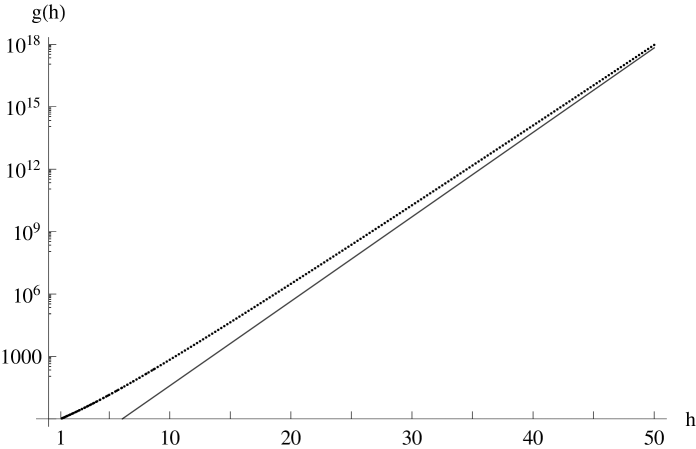
Figure 1: The black dots represent numerical evaluations of the function $g(h)$ given in eq. (3.12). The gray line is the function $a(8/\pi)^{h}$, with the coefficient $a$ fitted to numerical evaluations of $g(h)$ in the range $1.25\leq h\leq 60$.

When $h=1$, the first term (and only the first term) of the solution in (3.1) contributes to $\langle\phi,\Psi\rangle$. It is given by

$$\langle\phi,\Psi\rangle\,=\,-\int_{\frac{1}{2}}^{\infty}dx\int_{\frac{1}{2}}^{\infty}dy\,\frac{e^{1-x-y}}{\pi\sqrt{(x-\tfrac{1}{2})(y-\tfrac{1}{2})}}\,\Bigl{\langle}\,f\!\circ\!\phi(0)\,c(\partial\sigma_{L})\sigma_{R}(x)\,\Bigr{\rangle}_{{\cal W}_{x+y-1}}\,,$$ (3.13)

and we find

$$g(1)\,=1\,.$$ (3.14)

The leading behavior of $g(h)$ at $h\gg 1$ can be determined analytically. We note that the dominant contribution to $g(h)$ in this limit comes from the part of the integration region where the factor $|\ldots|^{h}$ in the integrand is maximized. It is easy to see that

$$\frac{2\sin\theta_{s}}{L\sin\theta_{x}\sin\theta_{y}}\,<\,\frac{8}{\pi}\,,$$ (3.15)

with the bound saturated at $x=y=\frac{1}{2}$ in the limit $s\to\infty$. We conclude that $g(h)$ behaves as

$$g(h)\,\sim\,\Bigl{(}\frac{8}{\pi}\Bigr{)}^{h}\qquad\text{ for }~{}~{}h\gg 1\,.$$ (3.16)

Figure 1 gives a plot of $g(h)$ on a logarithmic scale, together with the asymptote of its large-$h$ behavior.

4 Application to the rolling tachyon profile

The rolling tachyon solution represents the time-dependent process of D-brane decay [64, 65, 66, 67, 68, 69, 70, 71, 72, 73, 74, 13, 14]. It can be constructed by choosing $V(t)$ to be

$$V(t)=e^{\frac{1}{\sqrt{\alpha^{\prime}}}X^{0}}\!(t)\,.$$ (4.1)

For this choice, operator products $V(t_{1})\,V(t_{2})\,\ldots V(t_{n})$ are regular [13, 14]. For example, the leading term of $V(t)\,V(0)$ in the limit $t\to 0$ is given by

$$V(t)\,V(0)\sim|\,t\,|^{2}\,e^{\frac{2}{\sqrt{\alpha^{\prime}}}X^{0}}\!(0)\,.$$ (4.2)

We therefore have

$$\lim_{\epsilon\to 0}\,\exp\,\biggl{[}\,\lambda\int_{0}^{\epsilon}dt\,V(t)\,\biggr{]}=1\,,\quad\lim_{\epsilon\to 0}\,\exp\,\biggl{[}\,\lambda\int_{a}^{b}dt\,V(t)\,\biggr{]}\,\exp\,\biggl{[}\,\lambda\int_{b+\epsilon}^{c}dt\,V(t)\,\biggr{]}=\exp\,\biggl{[}\,\lambda\int_{a}^{c}dt\,V(t)\,\biggr{]}\,,$$ (4.3)

and thus the corresponding bcc operators satisfy the two conditions in (1.2). The magnitude of the deformation parameter $\lambda$ can be changed by time translation, so all solutions with the same sign of $\lambda$ are physically equivalent. In our convention the solution with $\lambda<0$ corresponds to the tachyon rolling to the direction of the tachyon vacuum without D-branes. The tachyon profile of the solution as a function of time $x^{0}$ takes the following form [13, 14]:

$$T(x^{0})=\sum_{n=1}^{\infty}\beta^{(n)}\,\lambda^{n}\,e^{\frac{1}{\sqrt{\alpha^{\prime}}}nx^{0}}\,.$$ (4.4)

The coefficients $\beta^{(n)}$ are obtained by evaluating

$$\begin{split}\beta^{(n)}\,\lambda^{n}=\langle\,\phi^{(n)},\Psi\,\rangle_{\rm density}\,,\end{split}$$ (4.5)

where

$$\phi^{(n)}(t)=-c\partial c\,\phi_{m}^{(n)}(t)\,,\qquad\phi_{m}^{(n)}(t)=e^{-\frac{n}{\sqrt{\alpha^{\prime}}}X^{0}}(t)\,.$$ (4.6)

Here and in what follows the subscript ‘density’ is used to denote the quantity divided by the spacetime volume. The weight $h$ of the operator $\phi_{m}^{(n)}(t)$ is given by $h=n^{2}$.

While the calculations of $\beta^{(n)}$ for the previous solutions [13, 14, 22] were complicated, the calculation of $\beta^{(n)}$ for (1.6) reduces to that of $C_{\phi}$. A convenient way to calculate $C_{\phi}$ is to take the following limit:

$$\begin{split}C_{\phi}&=\bigl{|}\,\tfrac{1}{2}(z+1)(z-1)\,\bigr{|}^{h}\,\bigr{\langle}\!\!\langle\,\phi_{m}(z)\,\sigma_{L}(-1)\,\sigma_{R}(1)\,\rangle\!\!\bigr{\rangle}_{\rm UHP}\\[2.15277pt] &=2^{-h}\lim_{z\to\infty}z^{2h}\,\bigr{\langle}\!\!\langle\,\phi_{m}(z)\,\sigma_{L}(-1)\,\sigma_{R}(1)\,\rangle\!\!\bigr{\rangle}_{\rm UHP}\,.\end{split}$$ (4.7)

The three-point function for $\phi_{m}^{(n)}$ is given by

$$\begin{split}\bigr{\langle}\!\!\langle\,\phi_{m}^{(n)}(z)\,\sigma_{L}(-1)\,\sigma_{R}(1)\,\rangle\!\!\bigr{\rangle}_{\rm UHP}&=\,\bigr{\langle}\!\!\langle\,\phi_{m}^{(n)}(z)\,\exp\,\biggl{[}\,\lambda\int_{-1}^{1}dt\,V(t)\,\biggr{]}\,\rangle\!\!\bigr{\rangle}_{\rm UHP}\\ &=\frac{\lambda^{n}}{n!}\int_{-1}^{1}dt_{1}\int_{-1}^{1}dt_{2}\ldots\int_{-1}^{1}dt_{n}\,\bigr{\langle}\!\!\langle\,\phi_{m}^{(n)}(z)\,V(t_{1})\,V(t_{2})\ldots V(t_{n})\,\rangle\!\!\bigr{\rangle}_{\rm UHP}\,.\end{split}$$ (4.8)

Since

$$\begin{split}&\bigr{\langle}\!\!\langle\,e^{-\frac{n}{\sqrt{\alpha^{\prime}}}\,X^{0}}\!(z)\,e^{\frac{1}{\sqrt{\alpha^{\prime}}}\,X^{0}}\!(t_{1})\,e^{\frac{1}{\sqrt{\alpha^{\prime}}}\,X^{0}}\!(t_{2})\,\ldots e^{\frac{1}{\sqrt{\alpha^{\prime}}}\,X^{0}}\!(t_{n})\,\rangle\!\!\bigr{\rangle}_{\rm UHP,\,density}~{}=~{}\prod_{i=1}^{n}\frac{1}{(z-t_{i})^{2n}}\,\prod_{i<j}(t_{i}-t_{j})^{2}\,,\end{split}$$ (4.9)

we obtain

$$C_{\phi^{(n)},\,{\rm density}}=\frac{\lambda^{n}}{2^{n^{2}}n!}\,I_{n}\,,$$ (4.10)

where

$$I_{n}=\int_{-1}^{1}dx_{1}\int_{-1}^{1}dx_{2}\ldots\int_{-1}^{1}dx_{n}\prod_{i<j}(x_{i}-x_{j})^{2}\,.$$ (4.11)

The integral $I_{n}$ is evaluated in appendix B, and we find

$$I_{n}=2^{n^{2}}n!\prod_{i=0}^{n-1}\frac{i!^{4}}{(2i+1)!(2i)!}\,.$$ (4.12)

It follows that

$$\boxed{\phantom{\biggl{(}}C_{\phi^{(n)},\,{\rm density}}=\lambda^{n}\prod_{i=0}^{n-1}\frac{i!^{4}}{(2i+1)!(2i)!}\,.~{}}$$ (4.13)

We can now study the large-$n$ behavior of $\beta^{(n)}$ analytically. We use Sterling’s approximation to find

$$C_{\phi^{(n)},\,{\rm density}}\,=\,\lambda^{n}\exp\Bigl{[}-2n^{2}\log 2+{\cal O}(n\log n)\Bigr{]}\,.$$ (4.14)

Combining this with the asymptotic behavior (3.16) of $g(h)$, we obtain

$$\beta^{(n)}=\exp\Bigl{[}-\gamma\,n^{2}+{\cal O}(n\log n)\Bigr{]}\,\qquad\text{with}~{}~{}\gamma\,=\,\log\frac{\pi}{2}\,.$$ (4.15)

It is obvious from this exponential suppression that the tachyon profile (4.4) converges at arbitrary time $x_{0}$. While numerical fits suggested convergence for the solution in [13, 14], the current solution allows an analytic proof of this convergence.

The resulting profile is highly oscillatory at large $x_{0}$. This feature of rolling tachyon solutions in string field theory was first observed in Siegel gauge by level truncation [67, 74] and later confirmed in Schnabl gauge by the analytic solution [13, 14]. While this peculiar behavior of the rolling tachyon had been a puzzle in string field theory, it was shown in [40] that the BCFT boundary state for the rolling tachyon studied by Sen [64] can be constructed from the solution in string field theory. It would be interesting to see if one can extract the closed string physics from the late-time behavior of our solution.

The oscillatory behavior in the rolling tachyon profile is linked to the appearance of a suppression factor $e^{-\gamma n^{2}}$ in the coefficients $\beta^{(n)}$. For the analytic solution [13, 14] in Schnabl gauge, the suppression factor was not analytically determined but numerically estimated in [13] as $n^{-0.38\,n^{2}}$ . For our solution based on bcc operators, we found $e^{-\gamma n^{2}}$ with $\gamma=\log(\pi/2)\approx 0.45$ . It is an interesting question if we can construct calculable analytic solutions without the dominant oscillatory behavior, i.e., solutions with $\gamma=0$. Let us consider the value of $\gamma$ for solutions associated with general projectors, which can be generated from our solution based on the sliver projector by reparameterizations [10]. As we mentioned before, the large-$h$ behavior of $g(h)$ is determined by considering $x=y=\frac{1}{2}$ in the limit $s\to\infty$ in (3.12). Combining this with (3.5), we find that $\gamma$ is determined from

$$\bigr{\langle}\!\!\langle\,\sigma_{R}(-\tfrac{1}{2})\,f\!\circ\!\phi_{m}(0)\,\sigma_{L}(\tfrac{1}{2})\,\rangle\!\!\bigr{\rangle}_{{\rm UHP}}=C_{\phi}\,\Bigl{(}\frac{8}{\pi}\Bigr{)}^{h}\,.$$ (4.16)

For $\phi=\phi^{(n)}$, this reproduces $\gamma=\log(\pi/2)$ as follows:

$$C_{\phi^{(n)},\,{\rm density}}\,\Bigl{(}\frac{8}{\pi}\Bigr{)}^{n^{2}}\sim\lambda^{n}\Bigl{(}\frac{2}{\pi}\Bigr{)}^{n^{2}}=\,\lambda^{n}\,e^{-\gamma n^{2}}\,.$$ (4.17)

We can use reparameterizations to generate new solutions, and then the function $f(\xi)$ in (2.3) is replaced by a general function $f(\xi)$ with $f(i)=\infty$ [10]. We usually choose $f(0)=0$ and $f(-1)=-f(1)$. The large-$h$ behavior is then determined by

$$\bigr{\langle}\!\!\langle\,\sigma_{R}(f(-1))\,f\!\circ\!\phi_{m}(0)\,\sigma_{L}(f(1))\,\rangle\!\!\bigr{\rangle}_{{\rm UHP}}=C_{\phi}\,\biggl{|}\frac{f^{\prime}(0)\,(f(1)-f(-1))}{(f(0)-f(1))\,(f(0)-f(-1))}\biggr{|}^{h}=C_{\phi}\,\biggl{(}\frac{2f^{\prime}(0)}{f(1)}\biggr{)}^{h}\,,$$ (4.18)

and $\gamma$ is given by

$$\gamma=\log\biggl{(}\frac{2f(1)}{f^{\prime}(0)}\biggr{)}\,.$$ (4.19)

For a generic choice of $f(\xi)$, the tachyon profile is not calculable, but it is calculable for solutions associated with special projectors [6]. A one-parameter family of special projectors labeled by $s$ with $s\geq 1$ was introduced in [6]. The associated function $f_{s}(\xi)$ and coefficient $\gamma_{s}$ are given by

$$f_{s}(\xi)\,=\,\xi\,{}_{2}F_{1}\bigl{[}\tfrac{s}{2},s;1+\tfrac{s}{2};-\xi^{2}\bigr{]}^{1/s}\,,\qquad~{}\gamma_{s}\,=\,\tfrac{1}{s}\log\!\frac{\sqrt{\pi}\,\Gamma\bigl{(}1+\tfrac{s}{2}\bigr{)}}{\Gamma\bigl{(}\tfrac{1}{2}+\tfrac{s}{2}\bigr{)}}\,.$$ (4.20)

The sliver projector corresponds to $s=1$, and the butterfly projector corresponds to $s=2$. The coefficient $\gamma_{s}$ for this family of solutions decreases as the parameter $s$ is increased. However, one cannot choose $s$ such that the dominant oscillatory behavior is absent. Indeed, $\gamma_{s}$ vanishes only in the limit $s\to\infty$, which corresponds to a singular limit of special projectors.

Appendix A Details of the derivation of $\Psi$

A.1 Derivation of (2.30)

We now derive the alternative form (2.30) of the solution $\Psi$ starting from (2.15). It is useful to note that

$$\frac{1}{1-h(K)\,BcV}=1-Bc+\frac{1}{1-h(K)\,V}\,Bc\,,$$ (A.1)

where $h(K)$ is an arbitrary function of $K$. This can be shown as follows:

$$\begin{split}\frac{1}{1-h(K)\,BcV}&=1+h(K)\,BcV+h(K)\,BcV\,h(K)\,BcV+\ldots\\ &=1+h(K)\,V\,Bc+h(K)\,V\,h(K)\,V\,Bc+\ldots\\ &=1-Bc+\frac{1}{1-h(K)\,V}\,Bc\,.\end{split}$$ (A.2)

It follows from

$$\biggl{[}\,1-B\,\frac{f(K)^{2}-1}{K}\,\lambda\,cV\,\biggr{]}^{-1}=1-Bc+\biggl{[}\,1-\frac{f(K)^{2}-1}{K}\,\lambda\,V\,\biggr{]}^{-1}Bc$$ (A.3)

and $cV\,(1-Bc)=0$ that

$$\begin{split}\Psi&=f(K)\,\lambda\,cV\,\biggl{[}\,1-\frac{f(K)^{2}-1}{K}\,\lambda\,V\,\biggr{]}^{-1}Bc\,f(K)\,.\end{split}$$ (A.4)

This is precisely the form of $\Psi$ presented in (2.30).

A.2 Derivation of $f(K)=1/\sqrt{1-K}$

Our starting point is the form (A.4) of the solution $\Psi$. We demand that the factor

$$\biggl{[}\,1-\frac{f(K)^{2}-1}{K}\,\lambda\,V\,\biggr{]}^{-1}$$ (A.5)

can be written in terms of wedges with insertions of finitely many bcc operators. In particular, we are interested in the case where it can be written as a sum over terms of the form

$$h_{1}(K+\lambda V)f_{1}(K)h_{2}(K+\lambda V)f_{2}(K)\ldots h_{k}(K+\lambda V)f_{k}(K)$$ (A.6)

with the functions $h_{i}$ (with finite index range $i=1,\ldots,k\leq\!k_{\rm max}\!<\!\infty$) of $K+\lambda V$ in the following form:

$$h_{i}(K+\lambda V)=\int_{0}^{\infty}d\alpha\,\tilde{h}_{i}(\alpha)\,\,e^{\alpha(K+\lambda V)}=\int_{0}^{\infty}d\alpha\,\tilde{h}_{i}(\alpha)\,\sigma_{L}\,e^{\alpha K}\,\sigma_{R}\,.$$ (A.7)

To write the factor (A.5) in the form (A.6), we use $\lambda V=(K+\lambda V)-K$ and obtain

$$\biggl{[}\,1-\frac{f(K)^{2}-1}{K}\,\lambda\,V\,\biggr{]}^{-1}\!\!=\biggl{[}\,f(K)^{2}-\frac{f(K)^{2}-1}{K}\,(K+\lambda\,V)\,\biggr{]}^{-1}\!\!=\sum_{k=0}^{\infty}\biggl{[}\frac{f(K)^{2}-1}{Kf(K)^{2}}\,(K+\lambda\,V)\,\biggr{]}^{k}\,f(K)^{-2}\,.$$ (A.8)

Each term in this sum is of the general form (A.6), with $h_{i}(K+\lambda V)=K+\lambda V$. Unfortunately, this is singular because

$$K+\lambda V=-\int_{-\infty}^{\infty}d\alpha\,\delta^{\prime}(\alpha)\,\sigma_{L}\,e^{\alpha K}\,\sigma_{R}\,,$$ (A.9)

which has support at $\alpha=0$ only. Consequently, all insertions of bcc operators collide, and no finite-width wedges with changed boundary conditions appear in the solution. In addition, this form does not have the uniform bound $k_{\rm max}$ on the number of bcc operators. However, if we have

$$\frac{f(K)^{2}-1}{Kf(K)^{2}}=a\,,$$ (A.10)

for some constant $a$ independent of $K$, then

$$\begin{split}\biggl{[}\,1-\frac{f(K)^{2}-1}{K}\,\lambda\,V\,\biggr{]}^{-1}&=\sum_{k=0}^{\infty}\bigl{[}\,a\,(K+\lambda\,V)\,\bigr{]}^{k}\,f(K)^{-2}=\frac{1}{1-a\,(K+\lambda V)}\,f(K)^{-2}\,.\end{split}$$ (A.11)

This expression is now a single term of the form (A.6), with $k=1$ , $h_{1}(x)=1/(1-ax)$ and $f_{1}(x)=f(x)^{-2}$. For $a>0$, $h_{1}$ has the smooth Laplace transform $\tilde{h}_{1}(\alpha)=a^{-1}e^{-\alpha/a}$, which vanishes at $\alpha\to\infty$. Thus (A.10), together with $a>0$, is the desired condition on $f(K)$. Solving it for $f(K)$, one obtains

$$f(K)=\frac{1}{\sqrt{1-aK}}\,.$$ (A.12)

In this case, we find $f_{1}(K)=1-aK$, which is also acceptable. We can use reparameterization [10] to transform $K$, $B$, $c$, and $V$ as

$$K\to\beta K\,,\qquad B\to\beta B\,,\qquad c\to\frac{1}{\beta}\,c\,,\qquad V\to\beta\,V\,.$$ (A.13)

If we choose $\beta=1/a$, we have

$$f(K)=\frac{1}{\sqrt{1-K}}\,,\qquad\Psi=\frac{1}{\sqrt{1-K}}\,\lambda\,cV\,\biggl{[}\,1-\frac{1}{1-K}\,\lambda\,V\,\biggr{]}^{-1}Bc\,\frac{1}{\sqrt{1-K}}\,.$$ (A.14)

This form is thus unique up to reparameterization.

Appendix B Evaluation of the integral $I_{n}$

In this appendix we evaluate the following integral:

$$I_{n}=\int_{-1}^{1}dx_{1}\int_{-1}^{1}dx_{2}\ldots\int_{-1}^{1}dx_{n}\prod_{i<j}(x_{i}-x_{j})^{2}\,.$$ (B.1)

The integral can be written as

$$I_{n}=\int_{-1}^{1}dx_{1}\int_{-1}^{1}dx_{2}\ldots\int_{-1}^{1}dx_{n}\,\Delta_{n}(x_{1},x_{2},\ldots,x_{n})^{2}\,,$$ (B.2)

where

$$\begin{split}\Delta_{n}(x_{1},x_{2},\ldots,x_{n})&\equiv\left|\begin{array}[]{cccccc}1&1&1&\ldots&1&1\\ x_{1}&x_{2}&x_{3}&\ldots&x_{n-1}&x_{n}\\ x_{1}^{2}&x_{2}^{2}&x_{3}^{2}&\ldots&x_{n-1}^{2}&x_{n}^{2}\\ \vdots&\vdots&\vdots&\ddots&\vdots&\vdots\\ x_{1}^{n-1}&x_{2}^{n-1}&x_{3}^{n-1}&\ldots&x_{n-1}^{n-1}&x_{n}^{n-1}\\ \end{array}\right|\,.\end{split}$$ (B.3)

Let us rewrite $\Delta_{n}(x_{1},x_{2},\ldots,x_{n})$ using the Legendre polynomials $P_{n}(x)$, which are given by

$$P_{n}(x)=\frac{1}{2^{n}n!}\,\frac{d^{n}}{dx^{n}}\,(x^{2}-1)^{n}\,,\qquad\int_{-1}^{1}dx\,P_{n}(x)\,P_{m}(x)=\frac{2}{2n+1}\,\delta_{nm}\,.$$ (B.4)

The normalized polynomials $\widehat{P}_{n}(x)$ defined by

$$\widehat{P}_{n}(x)\equiv\frac{1}{c_{n}}P_{n}(x)\qquad\text{ with }~{}~{}~{}c_{n}=\frac{1}{2^{n}n!}\,\frac{(2n)!}{n!}\,$$ (B.5)

have the form $\widehat{P}_{n}(x)=x^{n}+\ldots$ and satisfy

$$\int_{-1}^{1}dx\,\widehat{P}_{n}(x)\,\widehat{P}_{m}(x)=a_{n}\,\delta_{nm}\qquad\text{with }~{}~{}~{}a_{n}=\frac{2}{2n+1}\,\frac{1}{c_{n}^{2}}\,.$$ (B.6)

Then the determinant $\Delta_{n}(x_{1},x_{2},\ldots,x_{n})$ can be written as

$$\begin{split}\Delta_{n}(x_{1},x_{2},\ldots,x_{n})&=\left|\begin{array}[]{cccccc}\widehat{P}_{0}(x_{1})&\widehat{P}_{0}(x_{2})&\widehat{P}_{0}(x_{3})&\ldots&\widehat{P}_{0}(x_{n})\\ \widehat{P}_{1}(x_{1})&\widehat{P}_{1}(x_{2})&\widehat{P}_{1}(x_{3})&\ldots&\widehat{P}_{1}(x_{n})\\ \vdots&\vdots&\vdots&\ddots&\vdots\\ \widehat{P}_{n-1}(x_{1})&\widehat{P}_{n-1}(x_{2})&\widehat{P}_{n-1}(x_{3})&\ldots&\widehat{P}_{n-1}(x_{n})\\ \end{array}\right|\,,\end{split}$$ (B.7)

and we find

$$I_{n}=\int_{-1}^{1}dx_{1}\int_{-1}^{1}dx_{2}\ldots\int_{-1}^{1}dx_{n}\,\Delta_{n}(x_{1},x_{2},\ldots,x_{n})^{2}\,=\,n!\,\prod_{i=0}^{n-1}a_{i}\,=\,2^{n^{2}}n!\prod_{i=0}^{n-1}\frac{i!^{4}}{(2i+1)!(2i)!}\,.$$ (B.8)

It is easy to verify this formula when $n=1,2,3$ . An explicit evaluation of the integral (B.1) gives

$$I_{1}\,=\,2\,,\qquad I_{2}\,=\,\frac{8}{3}\,,\qquad I_{3}\,=\,\frac{64}{45}\,,$$ (B.9)

in agreement with (B.8).

References

- [1] E. Witten, “Noncommutative Geometry And String Field Theory,” Nucl. Phys. B 268, 253 (1986).
- [2] M. Schnabl, “Analytic solution for tachyon condensation in open string field theory,” Adv. Theor. Math. Phys. 10, 433 (2006) [arXiv:hep-th/0511286].
- [3] Y. Okawa, “Comments on Schnabl’s analytic solution for tachyon condensation in Witten’s open string field theory,” JHEP 0604, 055 (2006) [arXiv:hep-th/0603159].
- [4] E. Fuchs and M. Kroyter, “On the validity of the solution of string field theory,” JHEP 0605, 006 (2006) [arXiv:hep-th/0603195].
- [5] E. Fuchs and M. Kroyter, “Schnabl’s operator in the continuous basis,” JHEP 0610, 067 (2006) [arXiv:hep-th/0605254].
- [6] L. Rastelli and B. Zwiebach, “Solving open string field theory with special projectors,” JHEP 0801, 020 (2008) [arXiv:hep-th/0606131].
- [7] I. Ellwood and M. Schnabl, “Proof of vanishing cohomology at the tachyon vacuum,” JHEP 0702, 096 (2007) [arXiv:hep-th/0606142].
- [8] H. Fuji, S. Nakayama and H. Suzuki, “Open string amplitudes in various gauges,” JHEP 0701, 011 (2007) [arXiv:hep-th/0609047].
- [9] E. Fuchs and M. Kroyter, “Universal regularization for string field theory,” JHEP 0702, 038 (2007) [arXiv:hep-th/0610298].
- [10] Y. Okawa, L. Rastelli and B. Zwiebach, “Analytic solutions for tachyon condensation with general projectors,” arXiv:hep-th/0611110.
- [11] T. Erler, “Split string formalism and the closed string vacuum,” JHEP 0705, 083 (2007) [arXiv:hep-th/0611200].
- [12] T. Erler, “Split string formalism and the closed string vacuum. II,” JHEP 0705, 084 (2007) [arXiv:hep-th/0612050].
- [13] M. Schnabl, “Comments on marginal deformations in open string field theory,” Phys. Lett. B 654, 194 (2007) [arXiv:hep-th/0701248].
- [14] M. Kiermaier, Y. Okawa, L. Rastelli and B. Zwiebach, “Analytic solutions for marginal deformations in open string field theory,” JHEP 0801, 028 (2008) [arXiv:hep-th/0701249].
- [15] T. Erler, “Marginal Solutions for the Superstring,” JHEP 0707, 050 (2007) [arXiv:0704.0930 [hep-th]].
- [16] Y. Okawa, “Analytic solutions for marginal deformations in open superstring field theory,” JHEP 0709, 084 (2007) [arXiv:0704.0936 [hep-th]].
- [17] E. Fuchs, M. Kroyter and R. Potting, “Marginal deformations in string field theory,” JHEP 0709, 101 (2007) [arXiv:0704.2222 [hep-th]].
- [18] Y. Okawa, “Real analytic solutions for marginal deformations in open superstring field theory,” JHEP 0709, 082 (2007) [arXiv:0704.3612 [hep-th]].
- [19] I. Ellwood, “Rolling to the tachyon vacuum in string field theory,” JHEP 0712, 028 (2007) [arXiv:0705.0013 [hep-th]].
- [20] I. Kishimoto and Y. Michishita, “Comments on Solutions for Nonsingular Currents in Open String Field Theories,” Prog. Theor. Phys. 118, 347 (2007) [arXiv:0706.0409 [hep-th]].
- [21] E. Fuchs and M. Kroyter, “Marginal deformation for the photon in superstring field theory,” JHEP 0711, 005 (2007) [arXiv:0706.0717 [hep-th]].
- [22] M. Kiermaier and Y. Okawa, “Exact marginality in open string field theory: a general framework,” JHEP 0911, 041 (2009) [arXiv:0707.4472 [hep-th]].
- [23] T. Erler, “Tachyon Vacuum in Cubic Superstring Field Theory,” JHEP 0801, 013 (2008) [arXiv:0707.4591 [hep-th]].
- [24] L. Rastelli and B. Zwiebach, “The off-shell Veneziano amplitude in Schnabl gauge,” JHEP 0801, 018 (2008) [arXiv:0708.2591 [hep-th]].
- [25] M. Kiermaier and Y. Okawa, “General marginal deformations in open superstring field theory,” JHEP 0911, 042 (2009) [arXiv:0708.3394 [hep-th]].
- [26] O. K. Kwon, B. H. Lee, C. Park and S. J. Sin, “Fluctuations around the Tachyon Vacuum in Open String Field Theory,” JHEP 0712, 038 (2007) [arXiv:0709.2888 [hep-th]].
- [27] T. Takahashi, “Level truncation analysis of exact solutions in open string field theory,” JHEP 0801, 001 (2008) [arXiv:0710.5358 [hep-th]].
- [28] M. Kiermaier, A. Sen and B. Zwiebach, “Linear b-Gauges for Open String Fields,” JHEP 0803, 050 (2008) [arXiv:0712.0627 [hep-th]].
- [29] O. K. Kwon, “Marginally Deformed Rolling Tachyon around the Tachyon Vacuum in Open String Field Theory,” Nucl. Phys. B 804, 1 (2008) [arXiv:0801.0573 [hep-th]].
- [30] S. Hellerman and M. Schnabl, “Light-like tachyon condensation in Open String Field Theory,” arXiv:0803.1184 [hep-th].
- [31] I. Ellwood, “The closed string tadpole in open string field theory,” JHEP 0808, 063 (2008) [arXiv:0804.1131 [hep-th]].
- [32] T. Kawano, I. Kishimoto and T. Takahashi, “Gauge Invariant Overlaps for Classical Solutions in Open String Field Theory,” Nucl. Phys. B 803, 135 (2008) [arXiv:0804.1541 [hep-th]].
- [33] I. Y. Aref’eva, R. V. Gorbachev and P. B. Medvedev, “Tachyon Solution in Cubic Neveu-Schwarz String Field Theory,” Theor. Math. Phys. 158, 320 (2009) [arXiv:0804.2017 [hep-th]].
- [34] A. Ishida, C. Kim, Y. Kim, O. K. Kwon and D. D. Tolla, “Tachyon Vacuum Solution in Open String Field Theory with Constant B Field,” J. Phys. A 42, 395402 (2009) [arXiv:0804.4380 [hep-th]].
- [35] T. Kawano, I. Kishimoto and T. Takahashi, “Schnabl’s Solution and Boundary States in Open String Field Theory,” Phys. Lett. B 669, 357 (2008) [arXiv:0804.4414 [hep-th]].
- [36] M. Kiermaier and B. Zwiebach, “One-Loop Riemann Surfaces in Schnabl Gauge,” JHEP 0807, 063 (2008) [arXiv:0805.3701 [hep-th]].
- [37] E. Fuchs and M. Kroyter, “Analytical Solutions of Open String Field Theory,” arXiv:0807.4722 [hep-th].
- [38] M. Asano and M. Kato, “General Linear Gauges and Amplitudes in Open String Field Theory,” Nucl. Phys. B 807, 348 (2009) [arXiv:0807.5010 [hep-th]].
- [39] I. Kishimoto, “Comments on gauge invariant overlaps for marginal solutions in open string field theory,” Prog. Theor. Phys. 120, 875 (2008) [arXiv:0808.0355 [hep-th]].
- [40] M. Kiermaier, Y. Okawa and B. Zwiebach, “The boundary state from open string fields,” arXiv:0810.1737 [hep-th].
- [41] N. Barnaby, D. J. Mulryne, N. J. Nunes and P. Robinson, “Dynamics and Stability of Light-Like Tachyon Condensation,” JHEP 0903, 018 (2009) [arXiv:0811.0608 [hep-th]].
- [42] I. Y. Aref’eva, R. V. Gorbachev, D. A. Grigoryev, P. N. Khromov, M. V. Maltsev and P. B. Medvedev, “Pure Gauge Configurations and Tachyon Solutions to String Field Theories Equations of Motion,” JHEP 0905, 050 (2009) [arXiv:0901.4533 [hep-th]].
- [43] I. Kishimoto and T. Takahashi, “Numerical Evaluation of Gauge Invariants for -gauge Solutions in Open String Field Theory,” Prog. Theor. Phys. 121, 695 (2009) [arXiv:0902.0445 [hep-th]].
- [44] I. Ellwood, “Singular gauge transformations in string field theory,” JHEP 0905, 037 (2009) [arXiv:0903.0390 [hep-th]].
- [45] I. Y. Aref’eva, R. V. Gorbachev and P. B. Medvedev, “Pure Gauge Configurations and Solutions to Fermionic Superstring Field Theories Equations of Motion,” J. Phys. A 42, 304001 (2009) [arXiv:0903.1273 [hep-th]].
- [46] E. A. Arroyo, “Cubic interaction term for Schnabl’s solution using Pade approximants,” J. Phys. A 42, 375402 (2009) [arXiv:0905.2014 [hep-th]].
- [47] M. Kroyter, “Comments on superstring field theory and its vacuum solution,” JHEP 0908, 048 (2009) [arXiv:0905.3501 [hep-th]].
- [48] T. Erler and M. Schnabl, “A Simple Analytic Solution for Tachyon Condensation,” JHEP 0910, 066 (2009) [arXiv:0906.0979 [hep-th]].
- [49] E. Aldo Arroyo, “The Tachyon Potential in the Sliver Frame,” JHEP 0910, 056 (2009) [arXiv:0907.4939 [hep-th]].
- [50] F. Beaujean and N. Moeller, “Delays in Open String Field Theory,” arXiv:0912.1232 [hep-th].
- [51] E. A. Arroyo, “Generating Erler-Schnabl-type Solution for Tachyon Vacuum in Cubic Superstring Field Theory,” J. Phys. A 43, 445403 (2010) [arXiv:1004.3030 [hep-th]].
- [52] S. Zeze, “Tachyon potential in KBc subalgebra,” arXiv:1004.4351 [hep-th].
- [53] M. Schnabl, “Algebraic solutions in Open String Field Theory - a lightning review,” arXiv:1004.4858 [hep-th].
- [54] I. Y. Aref’eva and R. V. Gorbachev, “On Gauge Equivalence of Tachyon Solutions in Cubic Neveu-Schwarz String Field Theory,” arXiv:1004.5064 [hep-th].
- [55] S. Zeze, “Regularization of identity based solution in string field theory,” JHEP 1010, 070 (2010) [arXiv:1008.1104 [hep-th]].
- [56] E. A. Arroyo, “Comments on regularization of identity based solutions in string field theory,” arXiv:1009.0198 [hep-th].
- [57] T. Erler, “Exotic Universal Solutions in Cubic Superstring Field Theory,” arXiv:1009.1865 [hep-th].
- [58] L. Bonora, C. Maccaferri and D. D. Tolla, “Relevant Deformations in Open String Field Theory: a Simple Solution for Lumps,” arXiv:1009.4158 [hep-th].
- [59] A. Hashimoto and N. Itzhaki, “Observables of string field theory,” JHEP 0201, 028 (2002) [arXiv:hep-th/0111092].
- [60] D. Gaiotto, L. Rastelli, A. Sen and B. Zwiebach, “Ghost structure and closed strings in vacuum string field theory,” Adv. Theor. Math. Phys. 6, 403 (2003) [arXiv:hep-th/0111129].
- [61] L. Rastelli and B. Zwiebach, “Tachyon potentials, star products and universality,” JHEP 0109, 038 (2001) [arXiv:hep-th/0006240].
- [62] A. Bagchi and A. Sen, “Tachyon Condensation on Separated Brane-Antibrane System,” JHEP 0805, 010 (2008) [arXiv:0801.3498 [hep-th]].
- [63] M. R. Gaberdiel and B. Zwiebach, “Tensor constructions of open string theories I: Foundations,” Nucl. Phys. B 505, 569 (1997) [arXiv:hep-th/9705038].
- [64] A. Sen, “Rolling Tachyon,” JHEP 0204, 048 (2002) [arXiv:hep-th/0203211].
- [65] A. Sen, “Tachyon matter,” JHEP 0207, 065 (2002) [arXiv:hep-th/0203265].
- [66] A. Sen, “Time evolution in open string theory,” JHEP 0210, 003 (2002) [arXiv:hep-th/0207105].
- [67] N. Moeller and B. Zwiebach, “Dynamics with infinitely many time derivatives and rolling tachyons,” JHEP 0210, 034 (2002) [arXiv:hep-th/0207107].
- [68] F. Larsen, A. Naqvi and S. Terashima, “Rolling tachyons and decaying branes,” JHEP 0302, 039 (2003) [arXiv:hep-th/0212248].
- [69] N. D. Lambert, H. Liu and J. M. Maldacena, “Closed strings from decaying D-branes,” JHEP 0703, 014 (2007) [arXiv:hep-th/0303139].
- [70] M. Fujita and H. Hata, “Time dependent solution in cubic string field theory,” JHEP 0305, 043 (2003) [arXiv:hep-th/0304163].
- [71] D. Gaiotto, N. Itzhaki and L. Rastelli, “Closed strings as imaginary D-branes,” Nucl. Phys. B 688, 70 (2004) [arXiv:hep-th/0304192].
- [72] T. Erler, “Level truncation and rolling the tachyon in the lightcone basis for open string field theory,” arXiv:hep-th/0409179.
- [73] A. Sen, “Tachyon dynamics in open string theory,” Int. J. Mod. Phys. A 20, 5513 (2005) [arXiv:hep-th/0410103].
- [74] E. Coletti, I. Sigalov and W. Taylor, “Taming the tachyon in cubic string field theory,” JHEP 0508, 104 (2005) [arXiv:hep-th/0505031].