Magnetic Cycles and Meridional Circulation in Global Models of Solar Convection

Abstract

We review recent insights into the dynamics of the solar convection zone obtained from global numerical simulations, focusing on two recent developments in particular. The first is quasi-cyclic magnetic activity in a long-duration dynamo simulation. Although mean fields comprise only a few percent of the total magnetic energy they exhibit remarkable order, with multiple polarity reversals and systematic variability on time scales of 6-15 years. The second development concerns the maintenance of the meridional circulation. Recent high-resolution simulations have captured the subtle nonlinear dynamical balances with more fidelity than previous, more laminar models, yielding more coherent circulation patterns. These patterns are dominated by a single cell in each hemisphere, with poleward and equatorward flow in the upper and lower convection zone respectively. We briefly address the implications of and future of these modeling efforts.

1 Introduction

As the Solar and Heliospheric Observatory (SOHO) was undergoing its final stages of pre-launch preparations and as the telescopes of the Global Oscillations Network Group (GONG) were being deployed around the world, Juri Toomre looked ahead with characteristic vision and enthusiasm:

The deductions that will be made in the near future from the helioseismic probing of the solar convection zone and the deeper interior are likely to provide a stimulus and to in turn be challenged by the major numerical turbulence simulations now proceeding apace with the developments in high performance computing (Toomre & Brummell 1995).

In the fifteen years since, the Michelson Doppler Imager (MDI) onboard SOHO and the GONG network have provided profound insights into the dynamics of the solar convection zone (Christensen-Dalsgaard 2002; Gizon & Birch 2005; Howe 2009). Meanwhile, high-resolution simulations of solar and stellar convection have become indispensible tools in interpreting and guiding helioseismic investigations (Miesch & Toomre 2009; Nordlund et al.   2009; Rempel et al.   2009). Juri has played a leading role in both endeavors.

In particular, it was Juri who led a team of young students and postdocs to develop what was to become known as the ASH (Anelastic Spherical Harmonic) code (Clune et al.   1999; Miesch et al.   2000). In last decade ASH has provided many novel insights into the dynamics of solar and stellar interiors, including the intricate structure of global-scale turbulent convection, the subtle nonlinear maintenance of differential rotation and meridional circulation, and the complex generation of mean and turbulent magnetic fields through hydromagnetic dynamo action (Miesch et al.   2000, 2006, 2008; Elliott et al.   2000; Brun & Toomre 2002; Brun et al.   2004, 2005; Browning et al.   2004, 2006; Browning 2008; Brown et al.   2008, 2010a,b; Brun & Palacios 2009; Featherstone et al.   2009).

In this paper we briefly review two recent development in ASH modeling, focusing on the current Sun in particular. These include the generation of coherent, organized, quasi-cyclic mean magnetic fields in an otherwise turbulent convection zone (§2) and the delicate maintenance of the solar meridional circulation (§3). Section 4 is a brief summary and look to the future. For ASH models of other stars and epochs, see the contributions by Brown and Browning (these proceedings).

2 Magnetic Self-Organization in a Convective Dynamo

Recent ASH simulations of convective dynamos in rapidly-rotating solar-like stars have revealed remarkable examples of magnetic self-organization, forming coherent toroidal bands of flux referred to as magnetic wreathes (Brown, these proceedings). There are typically two wreaths centered at latitudes of approximately $\pm 20-30$ degrees, with opposite polarity in the northern and southern hemispheres. They persist amid the intense turbulence of the convection zone, maintained by the convectively-driven rotational shear. Two simulations in particular highlight the possible temporal evolution exhibited by such dynamos. In Case D3, rotating at three times the solar rate (rotation period $P_{rot}=$ 9.3 days), the wreathes persist indefinitely, buffeted by convective motions but otherwise stable for thousands of days (Brown et al.   2010a). In Case D5, rotating at five times the solar rate ($P_{rot}=$5.6 days), the wreathes undergo quasi-cyclic polarity reversals on a time scale of about 4 years (Brown et al.   2010b).

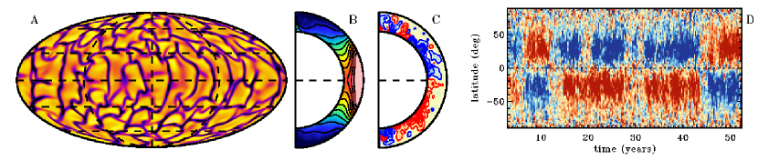
Figure 1: Dynamo action in a solar convection simulation. (A) Radial velocity field near the top of the convection zone ($r=0.96R$) in a Molleweide projection (yellow denotes upflow, blue/black downflow). (B) Angular velocity $\Omega$ and (C) toroidal magnetic field $\left<B_{\phi}\right>$, averaged over longitude and time (pink/blue denote fast/slow rotation, red/blue denote eastward/westward field). The time average for $\Omega$ spans the 50-year time interval shown while the time average for $\left<B_{\phi}\right>$ focuses on a 6-day interval near $t=25$ yr. (D) Longitudinally-averaged toroidal field $\left<B_{\phi}\right>$ at the base of the convection zone versus latitude and time. Saturation levels for the color tables are (A) $\pm$ 70 m s^-1, (B) 375–470 nHz, and (C,D) $\pm$ 3kG. Peak values of $\left<B_{\phi}\right>$ reach $\pm$ 10–14 kG.

Such behavior is dramatically different from early ASH simulations of convective dynamos at the current solar rotation rate ($P_{rot}=$ 28 days) by Brun et al. (2004). These were dominated by small-scale turbulent magnetic fields with complex, chaotic mean fields. The addition of a tachocline promoted the generation of stronger, more stable mean fields throughout the convection zone, with wreath-like equatorially antisymmetric toroidal bands in the stably-stratified region below the convection zone (Browning et al. 2006; Miesch et al. 2009). This tachocline simulation and a counterpart with different initial conditions (Browning et al. 2007) were run for 10-30 years each but no polarity reversals were observed.

Motivated by these previous studies, we initiated a new simulation in order to investigate whether self-organization processes comparable to those exhibited by the rapid rotators D3 and D5 might occur also at the solar rotation rate. In order to enable long time integration, we chose a moderate resolution of $N_{r}$, $N_{\theta}$, $N_{\phi}$ = 129, 256, 512. This is the same vertical resolution but half the horizontal resolution of Case M3 from Brun et al. (2004). The lower horizontal resolution required higher viscous, thermal, and magnetic dissipation but by having the eddy dffusivity scale as $\eta(r)\propto\hat{\rho}(r)^{-1}$ rather than $\eta(r)\propto\hat{\rho}(r)^{-1/2}$ as in case M3, we were able to achieve comparable values of $\eta$ at the base of the convection zone in the two cases; $\eta(r_{b})=2.03\times 10^{11}$ cm² s^-1 in Case M3 versus $\eta(r_{b})=2.88\times 10^{11}$ cm² s^-1 in the case reported presently, which we refer to as Case M4. Here $\hat{\rho}(r)$ is the background density profile and $r_{b}$ is the base of the convection zone.

Other than the horizontal resolution and dissipation, the principle difference between M3 and M4 is the lower magnetic boundary condition. Case M3 matched to a potential field whereas Case M4 employs a perfect conductor. This has large implications for mean field generation; we find that perfectly conducting boundary conditions promote the generation of strong toroidal fields in wreath-building dynamos such as D3 and D5. Furthermore, we have also imposed a latitudinal entropy gradient at the lower boundary as described by Miesch et al. (2006) in order to promote a solar-like, conical angular velocity profile. This takes into account thermal coupling to the expected dynamical force balance in the tachocline without explicitly including the tachocline itself, which requires fine spatial and temporal resolution. Omission of the tachocline may well have important consequences as to the nature of the dynamo, but we focus here on the generation of large-scale fields by turbulent convection and rotational shear in the solar envelope as an essential step toward understanding the fundamental elements of the solar dynamo.

Results for case M4 are illustrated in Figure 1. The convective patterns (A) are similar to previous simulations of comparable resolution and the differential rotation (B) is solar-like, with nearly conical mid-latitude contours and a monotonic decrease in angular velocity of about 25% from equator to pole (475 nHz - 370 nHz). In contrast to case M3, this simulation generates coherent layers of toroidal magnetic flux near the base of the convection zone, with opposite polarity in each hemisphere (C). As the simulation evolves, the polarity of these flux layers reverses several times (D). The characteristic time scale for reversals appears to be about 14-15 years, although there is a failed reversal at $t\approx 30$ yr. The more rapid reversals early in the simulations may represent initial transients as the dynamo is becoming established. The magnetic diffusion time scale $\tau_{\eta}\sim r^{2}\eta^{-1}\pi^{-2}$ ranges from 40 years at the inner boundary to 1.4 years at the outer boundary.

Given the generation of coherent mean fields, one might be tempted to refer to this as a large-scale dynamo (Brandenburg & Subramanian 2005). However, the magnetic energy spectrum does not peak at large scales, as one may expect from a turbulent $\alpha$-effect or an inverse cascade of magnetic helicity. Rather, the magnetic energy peaks on scales smaller than the velocity field, with mean fields making up only 3% of the total magnetic energy. This is in contrast to the wreath-building rapid rotators D3 and D5 where approximately half (46-47%) of the magnetic energy is in the mean fields.

In cases D3 and D5 the wreathes form and persist in the midst of the turbulent convection zone whereas in case M4 the coherent toroidal fields are confined to the base of the convection zone. This can be attributed largely to the relative strength of the rotational shear. In cases D3 and D5, the bulk of the kinetic energy (relative to the rotating frame) is in the differential rotation (65% and 71% respectively). The stronger shear in turn is a consequence of the stronger rotational influence, which promotes angular momentum transport by means of the Coriolis-induced Reynolds stress. In case M4 the rate at which the wreathes are generated by rotational shear is comparable to or larger than the rate at which they are destroyed by convective mixing. Here only 35% of the kinetic energy is in the differential rotation, with 65% in the convection (the meridional circulation accounts for less than 1% of the KE in all three cases). The rotational shear is not strong enough to sustain the wreathes in the mid convection zone and horizontal flux is pumped downward by turbulent convective plumes. Toroidal flux accumulates and persists near the base of the convection zone where the vertical velocity drops to zero and where it is further amplified by rotational shear. The depth dependence of $\eta$ also contributes to the localization of the wreathes near the base of the convection zone. As mentioned above, $\eta\propto\hat{\rho}^{-1}$ in case M4 whereas $\eta\propto\hat{\rho}^{-1/2}$ in cases D3 and D5.

It is notable that such toroidal flux layers develop even without a tachocline. In the penetrative simulations by Browning et al.  (2006) radial shear in the tachocline does contribute to the formation of persistent toroidal flux layers but case M4 demonstrates that latitudinal shear in the lower convection zone is sufficient. This is consistent with recent mean-field dynamo models which suggest that latitudinal shear in the lower convection zone is more effective at generating strong, latitudinally-extended toroidal flux layers than the radial shear in the tachocline (e.g. Dikpati & Gilman 2006).

Latitudinal shear is sufficient to generate toroidal flux layers at the base of the convection zone but are they strong enough to spawn the buoyant flux structures responsible for photospheric active regions? The peak strength of the mean toroidal field in case M4 reaches about 10⁴G. This is toward the lower end of estimated field strengths of 10⁴-10⁵G based on observations of bipolar active regions coupled with theoretical and numerical models of flux emergence (Fan 2004; Jouve & Brun 2009). However, local (pointwise) values of the longitudinal field $B_{\phi}$ typically reach 30-40kG in the magnetic layers and even stronger fields would be expected in higher-resolution simulations with less subgrid-scale diffusion. Convection may also promote the destabilization and rise of flux tubes, producing solar-like tilt angles of bipolar active regions even for relatively weak fields or order 15 kG (Weber et al.   2010). Case M4 does not exhibit buoyant flux structures, possibly due to insufficient resolution.

A prominent feature of the rapidly-rotating wreath-building dynamos D3 and D5 is an octupolar structure for the mean poloidal field (Brown 2010a,b). Poloidal separatrices lie at the poleward edge of the wreathes, although the magnetic topology can become more complex during reversals. By contrast, the mean poloidal field in case M4 is predominantly dipolar, often with weak, transient loops of opposite polarity at high latitudes.

We do not propose that this is a viable model of the solar dynamo. It does not exhibit equatorward-propagating activity bands or flux emergence comparable to active regions. Still, it is remarkable that the characteristic time scale for evolution of the mean fields is just over a decade, two orders of magnitude longer than the rotation period and the convection turnover time scale (both of order a month). Furthermore, quasi-cyclic polarity reversals occur on decadal time scales without flux emergence (required by the Babcock-Leighton mechanism), without a tachocline, and without significant flux transport by the meridional circulation. Cyclic variability on similar time scales was also found by Ghizaru et al. (2010) in convective dynamo simulations with a tachocline.

3 Maintenance of Meridional Circulation

With the recent surge in popularity of Flux-Transport solar dynamo models, the meridional circulation in the solar envelope has become a topic of great interest. According to the Flux-Transport paradigm, equatorward advection of torodial flux by the meridional circulation near the base of the solar convection zone is largely responsible for the observed butterfly diagram and thus regulates the time scale for the 22-year solar activity cycle (Dikpati & Gilman 2006; Rempel 2006; Jouve & Brun 2007; Charbonneau 2010). In the postulated advection-dominated regime under which many Flux-Transport models operate, the meridional circulation also dominates the transport of magnetic flux from the poloidal source region in the upper convection zone to the toroidal source region near the base of the convection zone.

Kinematic mean-field dynamo models cannot address how the solar meridional circulation is maintained; it is imposed as a model input. Non-kinematic mean-field models (e.g. Rempel 2005,2006) can give much insight into the underlying dynamics but they are necessarily based on theoretical models for the convective Reynolds stress, heat flux, and $\alpha$-effect that need to be verified. 3D Convection simulations are essential for a deeper understanding of how the solar meridional circulation is established and what its structure and evolution may be.

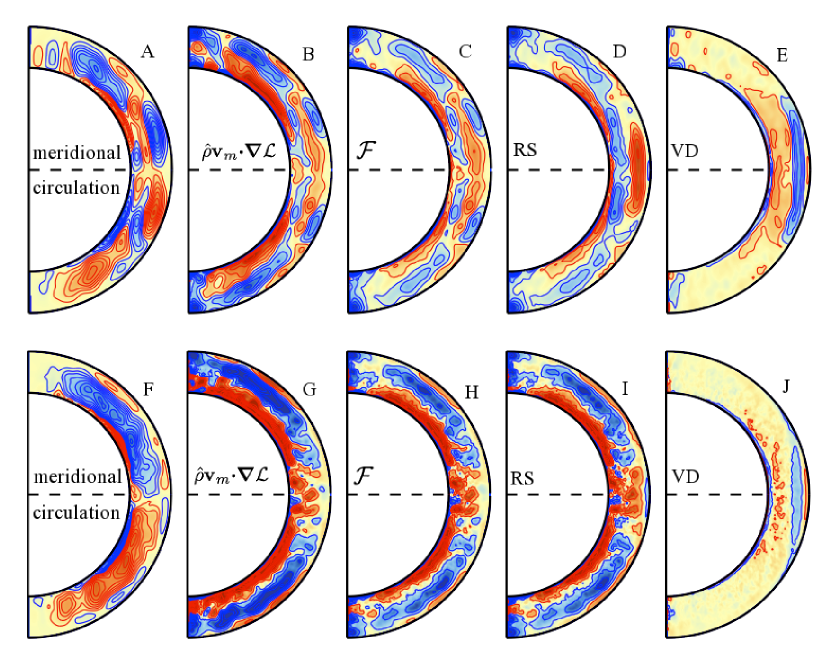
Figure 2: Maintenance of meridional circulation in two solar convection simulations. The top row (A–E) shows the dynamo simulation M4 discussed in §2 while the bottom row (F–J) shows a higher-resolution hydrodynamic simulation. Plotted are streamlines of the mass flux (A, F), the left (B,G) and right (C,H) hand sides of equation (1), and the contributions of the Reynolds stress (D,I) and the viscous diffusion (E,J) to the net torque ${\cal F}$, as expressed in eq. (3). All quantities are averaged over longitude and time (each over 300 days) and contour levels range from $\pm 2\times 10^{7}$ g cm^-1 s^-2 in (B–E) and $\pm 5\times 10^{6}$ g cm^-1 s^-2 in (G–J). Contour levels for the streamfunctions in (A) and (F) each range from $\pm 8\times 10^{21}$ g s^-1, corresponding to typical meridional flow speeds of order 20 m s^-1 and several m s^-1 in the upper and lower convection zone respectively. Red and blue denote positive and negative values, which correspond to clockwise and counter-clockwise circulations in (A) and (F).

The meridional circulation in the solar envelope is established in response to the convective angular momentum transport as follows

$$\left<\hat{\rho}{\bf v}_{m}\right>_{\phi,t}\mbox{\boldmath$\cdot$}\mbox{\boldmath$\nabla$}{\cal L}={\cal F}~{}~{}~{},$$ (1)

where $\hat{\rho}=\left<\rho\right>_{\phi,t}$ is the mean density stratification, ${\bf v}_{m}$ is the velocity in the meridional plane, and ${\cal L}$ is the specific angular momentum:

$${\cal L}=\lambda^{2}\Omega=r\sin\theta\left(r\sin\theta\Omega_{0}+\left<v_{\phi}\right>_{\phi,t}\right)~{}~{}~{}.$$ (2)

Angular brackets with subscripts $<>_{\phi,t}$ denote averages over longitude and time, $\Omega_{0}$ is the rotation rate of the rotating coordinate system. $\Omega$ is the net rotation rate (including differential rotation), and $\lambda=r\sin\theta$ is the moment arm. The net torque ${\cal F}$ includes components arising from the convective Reynolds stress (RS), viscous diffusion (VD), and the Lorentz Force:

$${\cal F}=-\mbox{\boldmath$\nabla\mbox{\boldmath$\cdot$}$}\left({\bf F}^{RS}+{\bf F}^{VD}+{\bf F}^{LF}\right)~{}~{}~{}.$$ (3)

where

$${\bf F}^{RS}=\hat{\rho}\lambda\left<{\bf v}_{m}^{\prime}v_{\phi}^{\prime}\right>_{\phi,t}~{}~{}~{},\mbox{\hskip 7.22743pt}{\bf F}^{VD}=-\hat{\rho}\lambda^{2}\nu\mbox{\boldmath$\nabla$}\Omega\mbox{\hskip 7.22743pt, and \hskip 7.22743pt}{\bf F}^{LF}=-\frac{\lambda}{4\pi}\left<{\bf B}_{m}B_{\phi}\right>_{\phi,t}~{}~{}~{}.$$ (4)

Here $\nu$ is the kinematic viscosity, ${\bf B}_{m}$ is the magnetic field in the meridional plane, and primes denote variations about the mean, e.g. $v_{\phi}^{\prime}=v_{\phi}-\left<v_{\phi}\right>_{\phi,t}$.

Note that equation (1) is derived from the zonal component of the momentum equation yet largely determines the meridional flow. A convergence (divergence) of angular momentum flux, yielding a positive (negative) torque ${\cal F}$, induces a meridional flow across ${\cal L}$ isosurfaces directed toward (away from) the rotation axis. This is the concept of gyroscopic pumping; for further discussion and references see Miesch & Toomre (2009).

The principle component of ${\cal F}$ responsible for maintaining the solar differential rotation and thus the meridional circulation via gyroscopic pumping is that due to the convective Reynolds stress ${\bf F}^{RS}$. The viscous component ${\bf F}^{VD}$ is negligible in the Sun. However, in numerical simulations viscous diffusion can largely oppose the convective Reynolds stress. The meridional circulation then responds only to the residual torque, adversely influencing its structure and evolution. This also holds in the presence of the Lorentz force. High resolution is required in order to minimize the artificial viscous diffusion and to therby achieve a more realistic zonal force balance.

The sensitivity of the meridional circulation profile to the zonal force balance is illustrated in Fig. 2 for two ASH convection simulations. The first (top row) is the moderate-resolution dynamo simulation M4 discussed in §2 ($N_{r}$, $N_{\theta}$, $N_{\phi}$ = 129, 256, 512). The second (bottom row) is a higher-resolution non-magnetic case with a lower viscosity that we will refer to as Case H ($N_{r}$, $N_{\theta}$, $N_{\phi}$ = 257, 512, 1024). The difference in $\nu$ is roughly a factor of four (mid convection zone values are $3.3\times 10^{12}$ cm² s^-1 for case M4 versus $0.80\times 10^{12}$ cm² s^-1 for case H, both varying with depth as $\hat{\rho}^{-1/2}$). Furthermore, the thermal diffusivity in case H is a factor of 2.7 less than in case M4 (mid convection zone values are $3.2\times 10^{12}$ cm² s^-1 and $8.7\times 10^{12}$ cm² s^-1, again varying as $\hat{\rho}^{-1/2}$).

Comparison of panel pairs $B$–$C$ and $G$–$H$ indicate that the dynamical balance expressed by eq. (1) is approximately satisfied. In both cases, the net torque ${\cal F}$ is given by summing up the contributions from the Reynolds stress and the viscous diffusion such that panel C $\approx$ D + E and panel H = I + J. The Lorentz force also contributes to the net torque in panel $C$ but its amplitude is small relative to the two terms shown (D,E).

There are two notable differences between the simulations M4 and H with regard to the maintenance of the meridional circulation. First, the nature of the Reynolds stress is different (D, I). Both simulations exhibit a convergence of ${\bf F}^{RS}$ at low latitudes that maintains the rotational shear but simulation H also exhbits a much more prominent inward angular momentum flux that is tending to accelerate the rotation in the lower convection zone relative to the upper convection zone. Furthermore, there is a radially outward angular momentum flux at low latitudes in case M4 that decelerates the lower convection zone. This is largely absent from case H. The second difference is the relative contribution of the viscous diffusion, which plays a smaller role in Case H due mainly to the smaller diffusivity $\nu$.

The net result of these two differences is that Case H exhibits a substantial positive (negative) torque at mid-latitudes in the lower (upper) convection zone. The dynamical balance achieved in eq. (1) then induces a coherent single-celled meridional circulation pattern with poleward flow in the upper convection zone and equatorward flow in the lower convection zone (F). By contrast, the radially outward Reynolds stress near the equator in case M4 and the opposing influence of viscous diffusion produce a weaker, less coherent net torque ${\cal F}$. The circulation patterns are consequently more complex, with multiple cells in radius and latitude (A).

The circulation pattern in Case H (panel F) is predominantly single-celled but exhibits narrow counter-cells near the boundaries. These are likely artifacts of the boundary conditions. At the bottom boundary we impose a latitudinal entropy gradient as discussed by Miesch et al. (2006) in order to take into account thermal coupling with the tachocline. We also impose stress-free boundaries so the total angular momentum in the shell is conserved. Although both boundary conditions are justified, they are incompatible with thermal wind balance whereby baroclinic and Coriolis-induced torques offset one another. The imbalance induces a clockwise (counter-clockwise) circulation in the northern (southern) hemisphere near the boundary. Penetrative convection simulations generally exhibit an equatorward circulation throughout the overshoot region, induced by the turbulent alignment of downflow plumes with the rotation axis (Miesch et al.  2000).

A more realistic upper boundary condition would include coupling to solar surface convection which includes granulation, mesogranulation and supergranulation. In lieu of the large Rossby number (rotation period relative to the convective turnover time), one may expect such surface convection to efficiently mix angular momentum, exerting a retrograde zonal torque (${\cal F}>0$). The presence of such a retrograde torque is implied by the existence of the near-surface shear layer, a subsurface increase in rotation rate ($\partial\Omega/\partial r<0$) detected in helioseismic inversions (Howe 2009). A retrograde torque in the solar surface layers would induce a poleward circulation according to eq. (1). Thus, the upper and lower counter-cells in the circulation profile of Fig. 2$F$ are likely artificial.

4 Summary and Outlook

Inspired by helioseismology and fueled by continuing advances in high-performance computing, global convection simulations continue to shape our understanding of solar internal dynamics and the solar dynamo. Recent simulations have achieved quasi-cyclic magnetic activity on decadal time scales and meridional circulation profiles that are qualitatively consistent with the single-celled circulation profiles assumed in many kinematic mean-field dynamo models. A more thorough discussion of these simulations and their implications will appear in forthcoming papers.

Further progress is imminent. The next decade may see the first global convective dynamo simulations that spontaneously generate buoyant magnetic flux structures from rotational shear that is self-consistently maintained by the convection itself, providing unprecedented insights into the origins of solar magnetic activity. Achieving this milestone will require numerical algorithms capable of exploiting next-generation computing architectures with 10⁵-10⁶ processing cores. It is a daunting but glorious challenge; one that Juri will surely relish.

This research is supported by NASA through Heliophysics Theory Program grants NNG05G124G and NNX08AI57G, and NASA SR&T grant NNH09AK14I, with additional support for Brown through NSF Astronomy and Astrophysics postdoctoral fellowship AST 09-02004. Browning was supported by CITA and Brun was partly supported by the Programme National Soleil-Terre of CNRS/INSU (France), and by the STARS2 grant from the European Research Council. The simulations were carried out with NSF PACI support of PSC, SDSC, TACC and NCSA, and by NASA HEC support at the NASA Advanced Supercomputing Division (NAS) facility at NASA Ames Research Center.

Appendix A Discussion

ROGERS: I don’t think counter-rotating cells at bottom boundary are entirely artificial because of hard boundaries, we see them in simulations with stable regions as well.

MIESCH: The sense of the meridional flow near the lower boundary arises from the stress-free mechanical boundary condition coupled to the imposed latitudinal entropy variation. Our 3D penetrative convection simulations generally have equatorward meridional flow in the overshoot region as a result of the turbulent alignment of downflow plumes and gyroscopic pumping associated with the convective angular momentum transport (Miesch et al.   2000). 2D simulations may exhibit different behavior. For further discussion, see the last two paragraphs of §3.

HUGHES: Do you think all the physics for magnetic buoyancy instability is incorporated in the anelastic approximation?

MIESCH: The essential assumption behind the anelastic approximation is that the Mach number is small. In order for this to break down in the deep solar interior within the context of flux emergence, it would imply MG fields and order-one thermal perturbations that can be ruled out by helioseismic structure inversions. The anelastic equation of state includes the influence of the pressure on density variations so it captures the physical mechanism underlying magnetic buoyancy. For a derivation of the Parker Instability in an anelastic system and nonlinear simulations of rising flux tubes see Fan (2001).

GOUGH: You commented that helioseismology indicates that the concentrated polar vortex hich you illustrated as a property of some your simulations poleward of about 85^′ does not exist. Actually that is not so: helioseismology has nothing to say so close to the axis of rotation. But it does indicate that the angular velocity poleward of 70 is lower than a smooth extrapolation would suggest- slow rotation in the region where the large scale dipole like magnetic field emanates and from which the fast component of the solar wind comes. Do you find any indications of that in the simulations?

MIESCH: The short answer is no. Some of our simulations have a monotonic decrease in the angular velocity $\Omega$ that continues to the poles and some exhibit a slight increase in $\Omega$ toward the poles. In the former solutions, the slope is rather smooth, with no indication of an abrupt steepening above 85^∘.

References

- [1] Brandenburg, A. & Subramanian, K. 2005, Phys. Rep., 417, 1
- [2] Brown, B.P., Browning, M.K., Brun, A.S., Miesch, M.S. & Toomre, J. 2008, ApJ, 689, 1354
- [3] Brown, B.P., Browning, M.K., Brun, A.S., Miesch, M.S. & Toomre, J. 2010, ApJ, 711, 424
- [4] Brown, B.P., Browning, M.K., Brun, A.S., Miesch, M.S. & Toomre, J. 2010, ApJ, submitted
- [5] Browning, M.K., Brun, A.S. & Toomre, J. 2004, ApJ, 601, 512
- [6] Browning, M.K., Miesch, M.S., Brun, A.S. & Toomre, J. 2006, ApJ Let., 648, L157
- [7] Browning, M.K., Brun, A.S., Miesch, M.S. & Toomre, J. 2007, Astron. Nachr., 328, 1100
- [8] Browning, M.K. 2008, ApJ, 676, 1262
- [9] Brun, A.S. & Toomre, J. 2002, ApJ, 570, 865
- [10] Brun, A.S., Miesch, M.S. & Toomre, J. 2004, ApJ, 614, 1073
- [11] Brun, A.S., Browning, M.K. & Toomre, J. 2005, ApJ, 629, 885
- [12] Brun, A.S. & Palacios, A. 2009, ApJ, 702, 1078
- [13] Charbonneau, P. 2010, LRSP, 7, http://www.livingreviews.org/lrsp-2010-3
- [14] Clune, T.L., Elliott, J.R., Miesch, M.S., Toomre, J., & Glatzmaier, G.A. 1999, Parallel Computing, 25, 361
- [15] Christensen-Dalsgaard, J. 2002, Rev. Mod. Phys., 74, 1073
- [16] Dikpati, M. & Gilman, P.A, 2006, ApJ, 649, 498
- [17] Eliott, J.R., Miesch, M.S. & Toomre, J. 2000, ApJ, 533, 546
- [18] Fan, Y. 2001, ApJ, 546, 509
- [19] Fan, Y. 2004, LRSP, 1, http://www.livingreviews.org/lrsp-2004-1
- [20] Featherstone, N.A., Browning, M.K., Brun, A.S. & Toomre, J. 2009, ApJ, 705, 1000
- [21] Ghizaru, M., Charbonneau, P. & Smolarkiewicz, P.K. 2010, ApJ Let., 715, L133
- [22] Gizon, L. & Birch, A.C. 2005, LRSP, 2, http://www.livingreviews.org/lrsp-2005-6
- [23] Howe, R. 2009, LRSP, 6, http://www.livingreviews.org/lrsp-2009-1
- [24] Jouve, L. & Brun, A.S. 2007, A&A, 474, 239
- [25] Jouve, L. & Brun, A.S. 2009, ApJ, 701, 1300
- [26] Miesch, M.S., Elliott, J.R., Toomre, J., Clune, T.L., Glatzmaier, G.A. & Gilman, P.A. 2000, ApJ, 532, 593
- [27] Miesch, M.S., Brun, A.S. & Toomre, J. 2006, ApJ, 641, 618
- [28] Miesch, M.S., Brun, A.S., DeRosa, M.L. & Toomre, J. 2008, ApJ, 673, 557
- [29] Miesch, M.S., Browning, M.K., Brun, A.S., Toomre, J. & Brown, B.P. 2009, in: M. Dikpati, T. Arentoft, I. González Hernández, C. Lindsey & F. Hill (eds.), Proc. GONG 2008/SOHO XXI Meeting on Solar-Stellar Dynamos as Revealed by Helio- and Asteroseismology, ASP Conf. Ser., vol. 416, p. 443
- [30] Miesch, M.S., & Toomre, J. 2009, Ann. Rev. Fluid Mech., 41, 317
- [31] Nordlund, A., Stein, R.F. & Asplund, M. 2009, LRSP, 6, http://www.livingreviews.org/lrsp-2005-2
- [32] Rempel, M. 2005, Ap.J., 622, 1320
- [33] Rempel, M. 2006, Ap.J., 647, 662
- [34] Rempel, M., Schüssler, M., Cameron, R.H. & Knölker 2009, Science, 325, 171.
- [35] Toomre, J., & Brummell, N.H. 1995, in: J.T. Hoeksema, V. Domingo, B. Fleck & B. Battrick (eds.), Fourth SOHO Workshop: Helioseismology (ESA: Noordwijk), p. 47
- [36] Weber, M, Fan, Y. & Miesch, M.S. 2010, in preparation