Local bifurcation-branching analysis
of global and “blow-up” patterns
for a fourth-order thin film equation

Abstract.

Countable families of global-in-time and blow-up similarity sign-changing patterns of the Cauchy problem for the fourth-order thin film equation (TFE–4)

$$\textstyle{u_{t}=-\nabla\cdot(|u|^{n}\nabla\Delta u)\quad\mbox{in}\quad\mathbb{R}^{N}\times\mathbb{R}_{+},\quad\mbox{where}\quad n>0,}$$

are studied. The similarity solutions are of standard “forward” and “backward” forms

$$\textstyle{u_{\pm}(x,t)=(\pm t)^{-\alpha}f(y),\quad y=x/(\pm t)^{\beta},\quad\beta=\frac{1-\alpha n}{4},\quad\pm t>0,\quad\mbox{where $f$ solve}}$$

(0.1) $$\textstyle{{\bf B}^{\pm}_{n}(\alpha,f)\equiv-\nabla\cdot(|f|^{n}\nabla\Delta f)\pm\beta y\cdot\nabla f\pm\alpha f=0\quad\mbox{in}\quad\mathbb{R}^{N},}$$

and $\alpha\in\mathbb{R}$ is a parameter (a “nonlinear eigenvalue”). The sign “$+$”, i.e., $t>0$, corresponds to global asymptotics as $t\to+\infty$, while “$-$” ($t<0$) yields blow-up limits $t\to 0^{-}$ describing possible “micro-scale” (multiple zero) structures of solutions of the PDE.

To get a countable set of nonlinear pairs $\{f_{\gamma},\alpha_{\gamma}\}$, a bifurcation-branching analysis is performed by using a homotopy path $n\to 0^{+}$ in (0.1), where ${\bf B}_{0}^{\pm}(\alpha,f)$ become associated with a pair $\{{\bf B},{\bf B}^{*}\}$ of linear non-self-adjoint operators

$$\textstyle{{\bf B}=-\Delta^{2}+\frac{1}{4}\,y\cdot\nabla+\frac{N}{4}\,I\quad\mbox{and}\quad{\bf B}^{*}=-\Delta^{2}-\frac{1}{4}\,y\cdot\nabla\quad(\mbox{so}\,\,\,({\bf B})^{*}_{L^{2}}={\bf B}^{*}),}$$

which are known to possess a discrete real spectrum, $\sigma({\bf B})=\sigma({\bf B}^{*})=\{\lambda_{\gamma}=-\frac{|\gamma|}{4}\}_{|\gamma|\geq 0}$ ($\gamma$ is a multiindex in $\mathbb{R}^{N}$). These operators occur after corresponding global and blow-up scaling of the classic bi-harmonic equation $u_{t}=-\Delta^{2}u$. This allows us to trace out the origin of a countable family of $n$-branches of nonlinear eigenfunctions by using simple or semisimple eigenvalues of the linear operators $\{{\bf B},{\bf B}^{*}\}$ leading to important properties of oscillatory sign-changing nonlinear patterns of the TFE, at least, for small $n>0$.

1. Introduction: TFE–4 and “adjoint” nonlinear eigenvalue problems

1.1. The model, two classes of similarity solutions, and main problems

In this paper, we study global asymptotic behaviour (as $t\to+\infty$) and finite-time blow-up behaviour (as $t\to T^{-}<+\infty$) of solutions of the fourth-order semilinear thin film equation (TFE-4)

(1.1) $$u_{t}=-\nabla\cdot(|u|^{n}\nabla\Delta u)\quad\mbox{in}\quad\mathbb{R}^{N}\times\mathbb{R}_{+},\quad n>0,$$

where $\nabla={\rm grad}_{x}$ and $\Delta=\nabla\cdot\nabla$ stands for the Laplace operator in $\mathbb{R}^{N}$.

Before describing the main application of such a nonlinear higher-order PDE model, which has become widely known in the last decades, we state the main goal of the paper. We study similarity solutions of (1.1) of two “forward” and Sturm’s “backward” types:

(i) global similarity patterns for $t\gg 1$, and

(ii) blow-up similarity ones with the finite-time behaviour as $t\to T^{-}<\infty$.

Both classes of such particular solutions of the TFE–4 (1.1) can be written in the joint form as follows (here, the blow-up time $T=0$ for solutions in (ii)):

(1.2) $$\textstyle{u_{\pm}(x,t)=(\pm t)^{-\alpha}f(y),\quad y=x/(\pm t)^{\beta}\,\,\,\mbox{for}\,\,\,\pm t>0,\quad\mbox{where}\quad\beta=\frac{1-\alpha n}{4},}$$

and similarity profiles $f(y)$ satisfy the following nonlinear eigenvalue problems, resp.,

(1.3) $$\framebox{$\textstyle{{\bf(NEP)_{\pm}}:\quad{\bf B}^{\pm}_{n}(\alpha,f)\equiv-\nabla\cdot(|f|^{n}\nabla\Delta f)\pm\beta y\cdot\nabla f\pm\alpha f=0\quad\mbox{in}\quad\mathbb{R}^{N}.}$}$$

Here, $\alpha\in\mathbb{R}$ is a parameter, which stands in both cases for admitted real nonlinear eigenvalues. Thus, the sign “$+$”, i.e., $t>0$, corresponds to global asymptotic as $t\to+\infty$, while “$-$” ($t<0$) yields blow-up limits $t\to T=0^{-}$ describing a “micro-scale” structure of the PDE. In fact, the blow-up patterns are assumed to describe the structures of “multiple zeros” of solutions of the TFE–4. This idea goes back to Sturm’s analysis of solutions of the 1D heat equation performed in 1836 [37]; see [24, Ch. 1] for the whole history and applications of these fundamental Sturm’s ideas and two zero set Theorems.

Being equipped with proper “boundary conditions at infinity”, namely,

(1.4) $$\mbox{for global case},\quad{\bf B}^{+}_{n}(\alpha,f):\quad f\in C_{0}(\mathbb{R}^{N})\quad(f\,\,\,\mbox{is compactly supported}),\quad\mbox{and}$$

(1.5) $$\mbox{for blow-up case},\quad{\bf B}^{-}_{n}(\alpha,f):\quad f(y)\,\,\,\mbox{has a ``minimal growth" as $y\to\infty$},$$

equations (1.3) become two true nonlinear eigenvalue problems to study, which can be considered as a pair of mutually “adjoint” ones. All related aspects and notions used above, remaining still somehow unclear, will be properly discussed and specified.

Our goal is to show by using any means that, for small $n>0$, eigenvalue problems

(1.6) $${\bf(NEP)_{\pm}} \Phi^{\pm}(n)=\{\alpha_{\gamma}^{\pm},f^{\pm}_{\gamma}\}_{|\gamma|\geq 0}$$ admit countable sets of solutions ,

where $\gamma$ is a multiindex in $\mathbb{R}^{N}$ to numerate the pairs.

The last question to address is whether these sets

(1.7) $$\mbox{ $\Phi^{\pm}(n)$ of nonlinear eigenfunctions are {\em evolutionary complete}},$$

i.e., describe all possible asymptotics as $t\to+\infty$ and $t\to 0^{-}$ (on the corresponding compact subsets in the variable $y$ in (1.2)) in the CP for the TFE–4 (1.1) with bounded compactly supported initial data.

Our main approach is the idea of a “homotopic deformation” of (1.1) as $n\to 0^{+}$ and reducing it to the classic bi-harmonic equation

(1.8) $$\textstyle{u_{t}=-\Delta^{2}u\quad\hbox{in}\quad\mathbb{R}^{N}\times\mathbb{R}_{+}\,,}$$

for which both problems (1.6) and (1.7) are solved positively by rather standard (but not self-adjoint) spectral theory of linear operators.

1.2. Main TFE applications: nonnegative and oscillatory solutions

It has been well known since the 1980s, when higher-order parabolic models began to be studied more actively, that the TFEs–4 like (1.1) have many applications arisen particularly in modeling the spreading of a liquid film along a surface, where $u$ stands for the height of the film in this context of thin film theory. Other physical related problems come from lubrication theory, nonlinear diffusion, flame and wave propagation (the Kuramoto–Sivashinsky equation and the extended Fisher–Kolmogorov equation), phase transition at critical Lifshitz points and bi-stable systems. We refer to a number of key survey and other papers on TFE theory such as [3, 4, 8, 9, 10, 12, 30]; see also Peletier–Troy [35] as a guide to higher-order ODEs and [19, 21] for most recent short surveys and long lists of references concerning physical derivations of various models, key mathematical results and applications of TFEs. Concerning mathematics of TFEs, one has to refer to the pioneering Bernis–Friedman paper [5] and [7, 23, 14] for the role of source-type similarity solutions of (1.1). On modern existence-uniqueness theory for the 1D TFE (for FBP setting), see [29], [20, § 6], and references therein.

It should be pointed out that most of the results cited above are associated with nonnegative solutions of a free-boundary problem (FBP) for the TFE–4 (1.1), while currently this equation is written for solutions of changing sign. Moreover, as mentioned above, the development of general approaches to nonnegative solutions of the FBP began with the work of Bernis–Friedman [5] in 1990 with such solutions having a most relevant physical motivation and applications.

The study of oscillatory solutions of changing sign for the TFE–4 is more recent; see [13, 20, 22] and references therein. It was shown in [19]–[22] (see also [1] as the most recent publication) that such solutions can be attributed to the Cauchy problem (CP) in $\mathbb{R}^{N}\times\mathbb{R}_{+}$, rather than a FBP, posed in a bounded domain with moving free boundaries. The study of the Cauchy problem is interesting from both points of view in some biological applications as well as its clear mathematical interest in PDE theory. We refer to [1], where more details on the CP setting are available.

In this connection, another pioneering paper of Bernis–McLeod in 1991 [6] should be mentioned, where existence and uniqueness of first three oscillatory source-type solutions of the Cauchy problem for the fourth-order porous medium equation (PME–4)

(1.9) $$u_{t}=-(|u|^{n}u)_{xxxx}\quad\hbox{in}\quad\mathbb{R}\times\mathbb{R}_{+}\,,$$

are studied. Here, unlike (1.1), equation (1.9) contains a monotone operator in the metric of $H^{-2}(\mathbb{R})$. By classic theory of monotone operators [33], the CP for (1.9) with compactly supported initial data $u_{0}$ admits a unique weak solution that is oscillatory close to the interfaces for all $n>0$ and evidently for $n=0$, where it becomes the bi-harmonic equation (1.8), with an oscillatory kernel of the fundamental solution; see below.

For $n>0$, such classes of the so-called “oscillatory solutions” of TFE–4 (1.1) is difficult to tackle rigorously, and even their ODE representatives (in the radial geometry) exhibit several surprises in trying to describe sign-changing features close to interfaces, [19]. Indeed, the CP in $\mathbb{R}^{N}\times\mathbb{R}_{+}$ shows compactly supported blow-up patterns, which have infinitely many oscillations near the interfaces and exhibit maximal regularity there (consult [19] for further details). It turns out that, for a better understanding of such singularity oscillatory properties of solutions of (1.1), it is quite fruitful to consider the homotopic limit $n\to 0^{+}$, thanks to the spectral theory developed for the pair $\{{\bf B},{\bf B}^{*}\}$ in [18] for rescaled operators where $n=0$. Thus, here we perform a homotopic approach, more rigorous than before, in order to obtain such interplay between the CP for the TFE-4 (1.1) and the bi-harmonic equation (1.8).

1.3. Our approach, problem setting, and layout of the paper

Before giving a description of our approaches, it is worth mentioning again that TFE theory for free boundary problems (FBPs) with nonnegative solutions is well understood nowadays (at least in 1D). The FBP setting assumes posing three standard boundary conditions at the interface, and such a theory has been developed in many papers since 1990. The mathematical formalities and general setting of the CP is still not fully developed and a number of problems remain open. In fact, the concept of proper solutions of the CP is still partially obscure, and moreover it seems that any classic or standard notions of weak-mild-generalized-… solutions fail in the CP setting.

Various ideas associated with extensions of smooth order-preserving semigroups are well known to be effective for second-order nonlinear parabolic PDEs, when such a construction is naturally supported by the maximum principle. The analysis of higher-order equations such as (1.1) is much harder than the corresponding second-order equations or those in divergent form (cf. (1.9)) because of the lack of the maximum principle, comparison, order-preserving, monotone, and potential properties of the quasilinear operators involved.

It is clear that the CP for the bi-harmonic equation (1.8) is well-posed and has a unique solution given by the convolution

(1.10) $$u(x,t)=b(x-\cdot,t)\,*\,u_{0}(\cdot),$$

where $b(x,t)$ is the fundamental solution of the operator $D_{t}+\Delta^{2}$. By the apparent connection between (1.1) and (1.8) (when $n=0$), intuitively at least, this analysis provides us with a way to understand the CP for the TFE-4 by using the fact that the proper solution of the CP for (1.1), with the same initial data $u_{0}$, is that one which converges to the corresponding unique solution of the CP for (1.8), as $n\rightarrow 0$. Thus, we shall use the patterns occurring for $n=0$, as branching points of nonlinear eigenfunctions, so some extra detailed properties of this linear flow will be necessary.

In Section 3, we, more carefully, introduce two classes of similarity solutions (the so-called nonlinear eigenfunctions), while Section 4 is devoted to necessary properties of the spectral pair $\{{\bf B},{\bf B}^{*}\}$ of linear differential operators that occur at $n=0$.

Our further analysis is as follows:

1.4. Local bifurcation-branching analysis for global solutions (Section 4): first operator theory discussion

In the first part of this work, we perform a local bifurcation-branching analysis with respect to the continuation parameter $n>0$, when that parameter is small enough. Thus, we obtain the bifurcation of solutions of the non-gradient equation $\eqref{eigpm}_{+}$ from the branch of the corresponding eigenfunctions of a rescaled linear operator. This yields some information and properties of the global in time similarity solutions $\eqref{upm}_{+}$ of the TFE–4 (1.1).

The linear elliptic equation occurring at $n=0$,

(1.11) $$\textstyle{{\bf B}F\equiv-\Delta_{y}^{2}F+\frac{1}{4}\,y\cdot\nabla_{y}F+\frac{N}{4}\,F=0\quad\hbox{in}\quad\mathbb{R}^{N},\quad\int\limits_{\mathbb{R}^{N}}F(y)\,{\mathrm{d}}y=1,}$$

where $F$ is the rescaled kernel of the fundamental solution $b(x,t)$ in (1.10), will be pivotal in the subsequent analysis. Indeed, the nonlinear operator in (1.3),

(1.12) $$\textstyle{{\bf B}_{n}^{+}(\alpha,f):=-\nabla\cdot(|f|^{n}\nabla\Delta f)+\frac{1-\alpha n}{4}\,y\cdot\nabla f+\alpha f,}$$

can be written in the following equivalent form:

(1.13) $$\textstyle{{\bf B}_{n}^{+}(\alpha,f)\equiv-\Delta^{2}f+\frac{1-\alpha n}{4}\,y\cdot\nabla f+\alpha f+\nabla\cdot((1-|f|^{n})\nabla\Delta f).}$$

Then, the solutions of ${\bf B}_{n}^{+}(\alpha,f)=0$ are regarded as steady states of the nonlinear evolution equation

(1.14) $$\textstyle{f_{\tau}={\bf B}_{n}^{+}(\alpha,f)\quad\mbox{in}\quad\mathbb{R}^{N}\times\mathbb{R}_{+}.}$$

The bifurcation-branching point from our solutions (for $n=0$) will be denoted by $(n,f)=(0,\psi_{k})$, which is shown to occur for some values of the nonlinear eigenvalue $\alpha$ written as $\alpha=\alpha_{k}$ ($k=|\beta|$ is characterized by a multiindex $\beta$ in $\mathbb{R}^{N}$), and $\psi_{k}$ representing the eigenfunctions of the operator ${\bf B}$, whose expressions will be obtained in detail later on.

Firstly, we shall prove that no bifurcation from the branch of trivial solutions $(n,f)=(0,0)$ occurs when the parameter $n$ approximates 0. Secondly, an infinite number of branches of solutions is shown to emanate from the eigenfunctions of the rescaled linear operator ${\bf B}$. Consequently, this analysis provides us with a countable family of solutions pairs (1.6) for the nonlinear equation $\eqref{eigpm}_{+}$ for small $n>0$.

According to classic bifurcation theory [15, 16, 31, 38], we denote

(1.15) $$\textstyle{{\bf B}_{n}^{+}(\alpha,f)\equiv\mathcal{F}(n,f):=\mathcal{L}(\alpha,n)f+\mathcal{N}(n,f),}$$

and assume that $n$ is the main continuation parameter. Then, in order to have a branch of solutions emanating from the branch of trivial solutions $(n,f)=(0,0)$ at certain values of the parameter $n$ (bifurcation points), the nonlinearity in (1.13), denoted by

$$\mathcal{N}(n,f):=\nabla\cdot((1-|f|^{n})\nabla\Delta f),$$

must fulfill the following conditions:

(1.16) $${\bf(NL):}\quad\textstyle{\mathcal{N}(n,0)=0,\quad D_{f}\mathcal{N}(n,0)=0\quad\hbox{for\,\, all}\quad n\in\mathbb{R}_{+}.}$$

In other words,

$$\mathcal{N}(n,f)=o(\left\|f\right\|)\quad\hbox{as}\quad f\rightarrow 0.$$

Recall that, here, $\mathcal{N}(n,f)$ serves as a perturbation of the operator ${\bf B}_{n}^{+}$ defined as in (1.13). Thus, under the given assumptions (which are not that easy to pose in a suitable functional setting, to say nothing of the proof), the linear operator denoted by

(1.17) $$\textstyle{\mathcal{L}(\alpha,n):=-\Delta^{2}+\frac{1-\alpha n}{4}\,y\cdot\nabla+\alpha I,}$$

defines an analytic semigroup in the space, where the solutions of $\eqref{eigpm}_{+}$ are defined.

Note that, in any case, the necessary assumptions for the nonlinearity of $\eqref{eigpm}_{+}$ are far from clearly specified, when $f$ is very close to zero, so something else must be imposed. Let us note that the condition (NL) in (1.16), roughly speaking, assumes that the functions $f(y)$ are sufficiently smooth and have “transversal” zeros with a possible accumulating point at a finite interface only. Otherwise, if $f(y)$ exhibits vanishing inside the support at a sufficiently “thick” nodal set, with many non-transversal zeros, this can undermine the validity of (1.16), even in any weak sense.

As customary in nonlinear operator theory, instead of the differential operators in (1.15), one has to deal with the equivalent integral equation

(1.18) $$f=-(\mathcal{L}(\alpha,n)-aI)^{-1}(\mathcal{N}(n,f)+af),$$

where $a>0$ is a parameter to be chosen so that the inverse operator (a resolvent value) is a compact one in a weighted space $L^{2}_{\rho}(\mathbb{R}^{N})$; see Section 3. We will show therein that the spectrum of $\mathcal{L}$ is always discrete and, actually,

(1.19) $$\textstyle{\sigma(\mathcal{L}(\alpha,n))=\big{\{}(1-\alpha n)\big{(}-\frac{k}{4}\big{)}+\alpha,\,k=0,1,2,...\big{\}},}$$

so that any choice of $a>0$ such that $a\not\in\sigma(\mathcal{L})$ is suitable in (1.18). Therefore, in particular, the conditions (1.16) are assumed to be valid in a weaker sense associated with the integral operator in (1.18).

Let us explain why a certain “transversality” of zeros of possible solutions $f(y)$ is of key importance. As we see from (1.13), we have to use the expansion for small $n>0$

(1.20) $$|f|^{n}-1\equiv{\mathrm{e}}^{n\,\ln|f|}-1=1+n\,\ln|f|+...-1=n\,\ln|f|+...\,,$$

which is true pointwise on any set $\{|f|\geq\varepsilon_{0}\}$ for an arbitrarily small fixed constant $\varepsilon_{0}>0$. However, in a small neighbourhood of any zero of $f(y)$, the expansion (1.20) is no longer true. Nevertheless, it remains true in a weak sense provided that this zero is sufficiently transversal in a natural sense, i.e.,

(1.21) $$\textstyle{\frac{|f|^{n}-1}{n}\rightharpoonup\ln|f|\quad\mbox{as}\quad n\to 0^{+}}$$

in $L^{\infty}_{\rm loc}$, since then the singularity $\ln|f(y)|$ is not more than logarithmic and, hence, is locally integrable in (1.18). Equivalently we are dealing with the limit

$$n\ln^{2}|f|\rightharpoonup 0,\quad\hbox{as}\quad n\downarrow 0^{+},$$

at least in a very weak sense, since by the expansion (1.20) we have that

$$\textstyle{\frac{|f|^{n}-1}{n}-\ln|f|=\frac{1}{2}\,n\,\ln^{2}|f|+...\,.}$$

Note also that actually we deal, in (1.18), with an easier expansion

(1.22) $$(|f|^{n}-1)\nabla\Delta f=(n\,\ln|f|+...)\nabla\Delta f,$$

so that even if $f(y)$ does not vanish transversally at a zero surface, the extra multiplier $\nabla\Delta f(y)$ in (1.22), which is supposed to vanish as well, helps to improve the corresponding weak convergence. Furthermore, it is seen from (1.13) that, locally in space variables, the operator in (1.18) (with $a=0$ for simplicity) acts like a standard Hammerstein–Uryson compact integral operator with a sufficiently smooth kernel:

(1.23) $$f\sim(\nabla\Delta)^{-1}[(|f|^{n}-1)\nabla\Delta f].$$

Therefore, in order to justify our asymptotic branching analysis, one needs in fact to introduce such a functional setting and a class of solutions

$$\mathcal{P}=\{f=f(\cdot,n):\,\,f\in H^{4}_{\rho}(\mathbb{R}^{N})\},$$

for which:

(1.24) $$\textstyle{{\mathcal{P}}:\quad\,\,(\nabla\Delta)^{-1}\big{(}\frac{|f|^{n}-1}{n}\,\nabla\Delta f\big{)}\to(\nabla\Delta)^{-1}(\ln\,|f|\nabla\Delta f)\quad\mbox{as}\quad n\to 0^{+}}$$

a.e. This is the precise statement on the regularity of possible solutions, which is necessary to perform our asymptotic branching analysis. In 1D or in the radial geometry in $\mathbb{R}^{N}$, (1.24) looks rather constructive. However, in general, for complicated solutions with unknown types of compact supports in $\mathbb{R}^{N}$, functional settings that can guarantee (1.24) are not achievable still. We mention again that, in particular, our formal analysis aims to establish structures of difficult multiple zeros of the nonlinear eigenfunctions $f_{\gamma}(y)$, at which (1.24) can be violated, but hopefully not in the a.e. sense.

To study nonlinear integral operators it is necessary to construct a function space in which the integral operator possesses favorable properties (continuity, compactness). Indeed, one can apply the classical fixed point principles of Schauder’s type to an operator acting between suitable Banach spaces. In this situation we can assert the existence of such fixed points establishing the continuity and boundedness of the integral operator. To do so, thanks to classical nonlinear integral operator theory we should impose the continuity of the kernel function involved in our integral operator (1.23).

Within the previous context, let us observe that the integral equation with a Hammerstein-Uryson operator-type (1.23) is equivalent to the integral equation (1.18), for which we know that the inverse operator $(\mathcal{L}(\alpha,n)-aI)^{-1}$ is compact. Indeed, by the spectral theory described in Section 3, we are able to deduce that the operator $\mathcal{L}$ is defined between two exponential weighted spaces. Hence, it looks like to ascertain the existence of such fixed points for (1.18) and, equivalently for (1.23), the suitable Banach spaces (that will provide us with the existence of solutions of the original equation (1.12)) are precisely those exponential weighted spaces, together with the assumption of continuity of the kernels involved in the equivalent integral equations (1.18) and (1.23).

In addition, we would like to mention that for the study of elliptic problems of order $2m$ by Schauder’s inversion procedure the suitable Banach spaces could be the typical pairs consisted of either Hölder spaces

$$\big{(}\mathcal{C}_{\rho}^{2m,\alpha}(\mathbb{R}^{N}),\mathcal{C}_{\rho}^{0,\alpha}(\mathbb{R}^{N})\big{)},\quad\hbox{with}\quad 0<\alpha<1,$$

or as remarked in the previous paragraph Sobolev spaces

$$\big{(}W_{\rho}^{2m,p}(\mathbb{R}^{N}),L_{\rho}^{p}(\mathbb{R}^{N})\big{)},\quad\hbox{with}\quad 1<p<\infty.$$

The particular weights assumed for those Banach spaces should be consistent with the exponential ones obtained in section 3. Thus, this enables us to obtain a priori estimates for the solutions of the original nonlinear equation (1.12) and provides us with the compactness of the integral operators involved in (1.18) and (1.23).

1.5. Regularity convention

Overall, we observe that, unlike classic existence bifurcation-branching theory [16, 31, 38], where sufficiently smooth expansions are used, the present singular one (1.20) dictates a special functional setting in a subset ${\mathcal{P}}$ of functions (admissible solutions), for which (1.24) should be valid a priori. In particular, such an analysis of the integral equation (1.18) will always require some deep knowledge of admissible structure of proper solutions $f(y)$ near zero (nodal) sets (also unknown), which we are still not aware of. Recall that, as our main goal, the present branching analysis is going to give us a first understanding of such delicate properties via the known eigenfunctions of the linear rescaled operators to appear at $n=0^{+}$.

Thus, since these necessary nodal properties of possible solutions $f(y)$ are unknown entirely rigorously, we perform our analysis under the following regularity convention:

$$\begin{array}[]{c}\text{{\em we assume that, regardless of the strong degeneracy of the nonlinear elliptic operator }}\\ \text{{\em involved, the problems under consideration in both integral and differential forms}}\\ \text{{\em admit sufficiently regular expansions of solutions in small $n>0$}}\\ \text{{\em in the functional class, for which \eqref{nn5} holds.}}\end{array}$$

As usual in bifurcation theory, the hypothesis for this to be valid is formulated for the equivalent integral representation of the operators, though, for simplicity, we perform the $n$-expansion analysis in the simpler (but indeed equivalent) differential form. Overall, currently, we honestly do not think that our analysis can be justified more rigorously than that: technicalities to arise can be extreme and a full prove truly illusive. However, in Appendix A, we show that a suitable justification of the branching is indeed achievable provided that clear transversality of a.a. zeros of linear eigenfunctions of ${\bf B}$ is known. Nevertheless, the problem of the actual existence of nonlinear eigenfunctions for small $n>0$ remains open still.

1.6. Further branching discussion

Now, once we have discussed the principal difficulties, which have arisen, we carry out a local bifurcation analysis close to $n=0$. Then, the change of stability from the branch of trivial solutions $(n,f)=(n,0)$ should be determined by the spectrum of the linearization $\mathcal{L}(\alpha,n)$ and the assumptions of the nonlinearity. Therefore, a bifurcation would take place at some values of the parameter $n$ if every neighbourhood of $(n,f)=(n,0)$ in $\mathbb{R}\times\mathcal{C}(\bar{\Omega})$ contains a nontrivial solution $(n,f)$ of $\eqref{eigpm}_{+}$ under the assumptions imposed for the linear and nonlinear part of the equation. However, as will be proved later, such a bifurcation from the branch of trivial solutions $(n,f)=(n,0)$ never happens at the value of the parameter $n=0$. Hence, we obtain a branching from the points $(n,f)=(0,\psi_{k})$ only; these arguments are fully consistent with more particular results obtained earlier in [1].

Moreover, since the bifurcation from the branch of trivial solutions depends on the eigenvalues of the linear operator (1.17), we believe that such a bifurcation does not exist at all (any proof is also very difficult). Indeed, after some rescaling of the type $y\mapsto ay$, with $a=(1-\alpha n)^{-1/4}$, it turns out that the spectrum of (1.17) is directly related to the spectrum of the linear operator ${\bf B}$. This suggests that no bifurcation from the branch of trivial solutions ever happens. Therefore, as also discussed in [1], we conjecture that if one wants to ascertain the global bifurcation analysis for these similarity TFEs-4, a new, different operator theory approach must be used.

Next, let us obtain the values of the parameter $\alpha$ for which the bifurcation-branching phenomena occurs. The spectrum of the operator ${\bf B}$ in (1.11), which appears for $n=0$ in $\eqref{eigpm}_{+}$, is already well known and will be explained in detail in the next sections. This has the form

$$\textstyle{\sigma({\bf B})=\big{\{}\lambda_{k}=:-\frac{k}{4}\,,\,k=0,1,2,...\big{\}}.}$$

Moreover, for $k=0$, i.e., for the first eigenvalue-eigenfunction pair $\{\alpha_{0}(n),f_{0}\}$, from the conservation of mass condition, denoting by $M(t)$ the mass of the solutions of (1.1), we have that (here $\Omega$ is the rescaled support of $f(y)$, however, for the CP, one can put $\Omega=\mathbb{R}^{N}$)

$$\textstyle{M(t):=\int\limits_{\Omega}u(x,t)\,{\mathrm{d}}x=t^{-\alpha}\int\limits_{\Omega}f(\frac{x}{t^{\beta}})\,{\mathrm{d}}x=t^{-\alpha+\beta N}\int\limits_{\Omega}f(y)\,{\mathrm{d}}y.}$$

This yields the exact values

(1.25) $$\textstyle{-\alpha+\beta N=0\quad\Longrightarrow\quad\alpha_{0}(n)=\frac{N}{4+Nn}\quad\mbox{and}\quad\beta_{0}(n)=\frac{1}{4+Nn}.}$$

However, the construction of the first eigenfunction $f_{0}(y)$ is not that straightforward even in 1D; see [20, § 7], where its oscillatory properties cease to exist at a heteroclinic bifurcation calculated numerically as

$$n_{\rm h}=1.7587...\,.$$

It is worth mentioning that, fortunately, for all $n\in(0,1)$ (this interval is of particular interest in what follows), both the existence and the uniqueness of $f_{0}(y)$ follow from the results of [6], since, rather surprisingly, source-type similarity profiles for (1.1) and (1.9) are reduced to each other with the parameter change $n\mapsto\frac{n}{n+1}$; see a precise statement in [20, Prop. 9.1].

Thus, it turns out that, when the parameter $n$ approximates zero, we obtain according to (1.25)

$$\textstyle{\alpha_{0}(0)=\frac{N}{4},}$$

so the solutions of $\eqref{eigpm}_{+}$ seem to approach the first eigenfunction $\psi_{0}$ associated with the first eigenvalue of the operator ${\bf B}$, i.e., corresponding to $\lambda_{0}=0$. However, that approximation for the solutions of $\eqref{eigpm}_{+}$ should also be extended to the eigenfunctions $\psi_{k}$, for any $k\geq 1$, when the parameter $\alpha$ reaches the following values:

(1.26) $$\textstyle{\alpha_{k}(0):=-\lambda_{k}+\frac{N}{4}\quad\hbox{for any}\quad k=1,2,\ldots,}$$

where $\lambda_{k}$ are the eigenvalues of the operator ${\bf B}$, so that

$$\textstyle{\alpha_{0}(0)=\frac{N}{4},\;\alpha_{1}(0)=\frac{N+1}{4},\;\alpha_{2}(0)=\frac{N+2}{4},\ldots,\alpha_{k}(0)=\frac{N+k}{4}\ldots\,.}$$

Then, we introduce the next expression for the parameter $\alpha$

(1.27) $$\textstyle{\alpha_{k}(n):=\frac{N}{4+Nn}-\lambda_{k}.}$$

Hence, due to the necessary assumptions, the structure of the bifurcating-branching set emanating at $(n,f)=(0,\psi_{k})$ depends on the spectral theory for the operator (1.11). For the first eigenvalue, since $\lambda_{0}=0$ is simple, we can ascertain accurately the local bifurcation-branching. Then, at least for sufficiently small $n$’s, the bifurcation-branching is locally a $\mathcal{C}^{1}$ curve, which can be parameterized as $s\mapsto(n_{0}(s),f(s))$ in $\mathbb{R}\times\mathcal{C}(\bar{\Omega})$ with

$$\textstyle{(n_{0}(0),f(0))=(0,\psi_{0}),\quad f^{\prime}(0)=\Phi_{0},\quad\Phi_{0}\in Y_{0}},$$

where ${}^{\prime}:=\frac{\mathrm{d}}{{\mathrm{d}}s}$, emanating from the eigenfunction $\psi_{0}$ at the $n=0$ in the direction of the space $Y_{0}$ orthogonal to the eigenspace $\ker\,{\bf B}$, with $\psi_{0}=F$ (the rescaled fundamental kernel of $b(x,t)$) being the eigenfunction associated with the eigenvalue $\lambda_{0}=0$.

However, in the case when the multiplicity of the eigenvalues $\lambda_{k}$ with $k\geq 1$ is higher (bigger than 1), we obtain that the continua emanating at $(n,f)=(0,\psi_{k})$ are tangent to the manifolds $Y_{k}$, orthogonal to $\ker\big{(}{\bf B}+\frac{k}{4}\,I\big{)}$. And, hence, we might have more than one direction of bifurcation-branching, depending on certain values related to the eigenfunctions which generate the eigenspace. This certainly agrees with the work of Rabinowitz [36], in which for potential operators and bifurcation from the branch of trivial solutions, one of the next alternatives for the bifurcation structure must be obtained:

(i) for the value of the parameter where the bifurcation takes place, the trivial solution is not isolated; or

(ii) for any other value of the parameter in one-sided neighbourhood of the bifurcation point, there are at least two nontrivial solutions; or

(iii) for any other value of the parameter in a neighbourhood of the bifurcation point, at least one nontrivial solution exists.

In general, the question about how many precise branches bifurcates for any $k\geq 1$ remains an open problem, though we think it is very related to the dimensions of the eigenspaces. As far as we know, only partial and very specific results have been obtained for non-variational problems with higher multiplicities.

1.7. Blow-up patterns via branching theory (Section 5)

This is a natural counterpart of the global similarity analysis of PDEs in the limits as $t\to\infty$. We next consider blow-up limits as $t\to T^{-}<\infty$, or $t\to 0^{-}$ as in $\eqref{upm}_{-}$, where $T=0$. We thus perform a detailed and systematic analysis of the blow-up similarity solutions. This is done again by using the homotopic approach as $n\to 0^{+}$ via branching theory, but this time based on the Lyapunov–Schmidt methods in order to obtain relevant results and properties for the solutions of the self-similar equation $\eqref{eigpm}_{-}$. This homotopic-like approach is based upon the spectral properties of the adjoint (to the ${\bf B}$ above) operator

(1.28) $$\textstyle{{\bf B}^{*}=-\Delta^{2}-\frac{1}{4}\,y\cdot\nabla,\quad\mbox{with}\quad\sigma({\bf B}^{*})=\big{\{}\lambda_{\beta}=-\frac{|\beta|}{4},\,\,|\beta|=0,1,2,...\big{\}},}$$

which occurs after blow-up scaling of the linear counterpart (1.8) of the TFE-4 (1.1) for $n=0$. Note that (1.28) admits a complete and closed set of eigenfunctions being generalized Hermite polynomials, which exhibit finite oscillatory properties.

It is curious that, in [19], blow-up similarity analysis of the related unstable TFE–4 did not detect any stable oscillatory behaviour of solutions near the interfaces of the radially symmetric associated equation. All the blow-up patterns turned out to be nonnegative, which is a specific feature of the PDE under consideration therein. This does not mean that blow-up similarity solutions of the CP do not change sign near the interfaces or inside the support. Actually, it was pointed out that local sign-preserving property could be attributed only to the blow-up ODE and not to the whole PDE (1.1). Hence, the possibility of having oscillatory solutions cannot be ruled out for every case. Indeed, thanks to the polynomial expressions of the eigenfunctions for the operator ${\bf B}^{*}$, we have, in particular, that the first eigenfunction $\psi^{*}(y)=1$ is not oscillatory, but for some other eigenfunctions we shall expect sign-changing behaviour.

Then, this homotopy study exhibits a typical difficulty concerning the desired structure of the transversal zeros of solutions, at least for small $n>0$. Proving such a transversality zero property is still a difficult open problem, though qualitatively, this was rather well understood in 1D and radial geometry, [19].

1.8. TFE: FBP and CP problem settings

We recall that, for both the FBP and the CP of (1.1), the solutions are assumed to satisfy standard free-boundary conditions:

(1.29) $$\left\{\begin{array}[]{ll}\textstyle{u=0,}&\textstyle{\hbox{zero-height,}}\\ \textstyle{\nabla u=0,}&\textstyle{\hbox{zero contact angle,}}\\ \textstyle{-{\bf n}\cdot\nabla(\left|u\right|^{n}\Delta u)=0,}&\textstyle{\hbox{conservation of mass (zero-flux)}}\end{array}\right.$$

at the singularity surface (interface) $\Gamma_{0}[u]\equiv\partial\Omega$, which is the lateral boundary of

$$\textstyle{\hbox{supp}\;u\subset\mathbb{R}^{N}\times\mathbb{R}_{+},\quad N\geq 1\,,}$$

where ${\bf n}$ stands for the unit outward normal to $\Gamma_{0}[u]$, which is assumed to be sufficiently smooth (the treatment of such hypotheses is not any goal of this paper). For smooth interfaces, the condition on the flux can be read as

$$\lim_{\hbox{dist}(x,\Gamma_{0}[u])\downarrow 0}-{\bf n}\cdot\nabla(|u|^{n}\Delta u)=0.$$

For the FBP, dealing with nonnegative solutions, this setting is assumed to define a unique solution. However, this uniqueness result is known in 1D only; see [29], where the interface equation was included into the problem setting. We also refer to [20, § 6.2], where a “local” uniqueness is explained via von Mises transformation, which fixes the interface point. For more difficult, non-radial geometries in $\mathbb{R}^{N}$, there is no hope of getting any uniqueness for the FBP, in view of possible very complicated shapes of supports leading to various “self-focusing” singularities of interfaces at some points, which can dramatically change the required regularity of solutions.

For the CP, the assumption on nonnegativity is got rid of, and solutions become oscillatory close to interfaces. It is then key that the solutions are expected to be “smoother” at the interface than those for the FBP, i.e., (1.29) are not sufficient to define their regularity. These maximal regularity issues for the CP, leading to oscillatory solutions, are under scrutiny in [20]; see also [1], as the most recent source of such a study.

Next, denote by

$$\textstyle{M(t):=\int u(x,t)\,{\mathrm{d}}x}$$

the mass of the solution, where integration is performed over smooth support ($\mathbb{R}^{N}$ is allowed for the CP only). Then, differentiating $M(t)$ with respect to $t$ and applying the divergence theorem (under natural regularity assumptions on solutions and free boundary), we have that

$$\textstyle{J(t):=\frac{{\mathrm{d}}M}{{\mathrm{d}}t}=-\int\limits_{\Gamma_{0}\cap\{t\}}{\bf n}\cdot\nabla(|u|^{n}\Delta u)\,.}$$

The mass is conserved if $J(t)\equiv 0$, which is assured by the flux condition in (1.29).

The problem is completed with bounded, smooth, integrable, compactly supported initial data

(1.30) $$\textstyle{u(x,0)=u_{0}(x)\quad\hbox{in}\quad\Gamma_{0}[u]\cap\{t=0\}.}$$

In the CP for (1.1) in $\mathbb{R}^{N}\times\mathbb{R}_{+}$, one needs to pose bounded compactly supported initial data (1.30) prescribed in $\mathbb{R}^{N}$. Then, under the same zero flux condition at finite interfaces (to be established separately), the mass is preserved; however smoother regularity properties of solutions require a separate study/understanding; see [20] for some results.

2. Self-similar solutions: two nonlinear eigenvalue problems

2.1. Global similarity solutions

We now more carefully derive the problem for global self-similar solutions of (1.1), which occur due to its natural scaling-invariant nature. Namely, using the following scaling in (1.1):

(2.1) $$\begin{matrix}x:=\mu\bar{x},\quad t:=\lambda\bar{t},\quad u:=\nu\bar{u},\quad\mbox{with}\vskip 3.0pt plus 1.0pt minus 1.0pt\vskip 3.0pt plus 1.0pt minus 1.0pt\\ \textstyle{\frac{\partial u}{\partial t}=\frac{\nu}{\lambda}\frac{\partial\bar{u}}{\partial\bar{t}},\quad\frac{\partial u}{\partial x_{i}}=\frac{\nu}{\mu}\frac{\partial\bar{u}}{\partial\bar{x}_{i}},\quad\frac{\partial^{2}u}{\partial x_{i}^{2}}=\frac{\nu}{\mu^{2}}\frac{\partial^{2}\bar{u}}{\partial\bar{x}_{i}^{2}},}\end{matrix}$$

and substituting those expressions in (1.1) yields

$$\textstyle{\frac{\nu}{\lambda}\frac{\partial\bar{u}}{\partial\bar{t}}=-\frac{\nu^{n+1}}{\mu^{4}}\nabla\cdot(|\bar{u}|^{n}\nabla\Delta\bar{u})\,.}$$

To keep this equation invariant, the following equalities must be fulfilled:

(2.2) $$\begin{matrix}\textstyle{\frac{\nu}{\lambda}=\frac{\nu^{n+1}}{\mu^{4}}\quad\Longrightarrow\quad}\mu:=\lambda^{\beta}\Longrightarrow\nu:=\lambda^{\frac{4\beta-1}{n}},\quad\mbox{so that}\vskip 3.0pt plus 1.0pt minus 1.0pt\vskip 3.0pt plus 1.0pt minus 1.0pt\\ \textstyle{u(x,t):=\lambda^{\frac{4\beta-1}{n}}\bar{u}(\bar{x},\bar{t})=\lambda^{\frac{4\beta-1}{n}}\bar{u}(\frac{x}{\mu}),\quad\mbox{where}\quad t=\lambda.}\end{matrix}$$

Consequently, we have to rescale in the following way:

(2.3) $$\textstyle{u_{+}(x,t)=t^{-\alpha}v(y,\tau),\quad y:=\frac{x}{t^{\beta}},\quad\tau=\ln t\,:\,\mathbb{R}_{+}\rightarrow\mathbb{R},\quad\mbox{where}\quad\,\,\,\beta=\frac{1-\alpha n}{4},}$$

such that $f(y,\tau)=\bar{u}(\frac{x}{t^{\beta}},\tau)$, we obtain, after substituting (2.3) into (1.1) and rearranging terms, that $f$ solves a quasilinear evolution equation given by

(2.4) $$\textstyle{v_{\tau}={\bf B}^{+}_{n}(\alpha,v)\equiv-\nabla\cdot(\left|v\right|^{n}\nabla\Delta v)+\frac{1-\alpha n}{4}\,y\cdot\nabla v+\alpha v\quad\mbox{in}\quad\mathbb{R}^{N}\times\mathbb{R}_{+}\,.}$$

Consider the steady-states of the parabolic equation (2.4). Thus, we analyze the local bifurcation-branching behaviour of the nonlinear eigenvalue problem:

(2.5) $$\framebox{$\textstyle{{\bf B}^{+}_{n}(\alpha,f)\equiv-\nabla\cdot(|f|^{n}\nabla\Delta f)+\frac{1-\alpha n}{4}\,y\cdot\nabla f+\alpha f=0,\quad f\in C_{0}(\mathbb{R}^{N})\,.}$}$$

Here, the “boundary conditions at infinity” stated as $f\in C_{0}(\mathbb{R}^{N})$ are naturally associated with the known properties of finite propagation for TFEs, which have been mathematically justified about two decades ago at least; see a survey on energy methods in PDE theory in [28]. Then, any assumption stating that $f(y)$ is “sufficiently small” at infinity, e.g.,

(2.6) $$f\in H^{4}(\mathbb{R}^{N})\quad\mbox{or}\quad H^{4}_{\rho}(\mathbb{R}^{N})$$

(the last space is a domain of the linear operator ${\bf B}$ in (1.11); see the next section), would lead to compactly supported solutions. In fact, such a conclusion entirely depends on asymptotic (i.e., local, not any global) properties of the nonlinear elliptic operators involved, so will not be a main concern in our study.

2.2. Blow-up similarity solutions

The blow-up similarity solutions of the TFE–4 (1.1) correspond to completely different limits and then describe a “micro-scale” structure of its solutions at any given point. For convenience, we reduce the blow-up time to $T=0$. Then, similar to the global solutions, replacing $t\mapsto(-t)$, we obtain the patterns

(2.7) $$\textstyle{u_{-}(x,t):=(-t)^{-\alpha}f(y),\quad y=\frac{x}{(-t)^{\beta}},\quad\hbox{with the same parameter}\quad\beta=\frac{1-\alpha n}{4}.}$$

Hence, substituting that expression into (1.1) and rearranging terms, we arrive at the following quasilinear elliptic equation:

(2.8) $$\framebox{${\bf B}_{n}^{-}(\alpha,f)\equiv-\nabla\cdot(|f|^{n}\nabla\Delta f)-\beta y\cdot\nabla f-\alpha f=0\quad\mbox{in}\quad\mathbb{R}^{N}.$}$$

In order to get the corresponding second “adjoint” nonlinear eigenvalue problem, one needs to specify a “minimal growth” of admissible nonlinear eigenfunctions $f(y)$ as $y\to\infty$. This will be done in Section 5. Note that, by obvious and straightforward reasons, (2.8) does not admit compactly supported solutions. Indeed, the nature of blow-up scaling (2.7) would then mean disappearance of a such a solution in finite time, contradicting uniqueness and other easy asymptotic issues for the TFE–4.

In general, for solutions with finite blow-up time $T\in\mathbb{R}$, the full self-similar scaling

(2.9) $$\textstyle{u(x,t)=(T-t)^{-\alpha}w(y,\tau),\quad y:=\frac{x}{(T-t)^{\beta}},\quad\tau=-\ln(T-t)\,:\,(-\infty,T)\rightarrow\mathbb{R},}$$

yields the parabolic equation

(2.10) $$\textstyle{w_{\tau}={\bf B}^{-}_{n}(\alpha,w)\equiv-\nabla\cdot(\left|w\right|^{n}\nabla\Delta w)-\frac{1-\alpha n}{4}\,y\cdot\nabla w-\alpha w\quad\mbox{in}\quad\mathbb{R}^{N}\times\mathbb{R}_{+}.}$$

3. Spectral properties of the linear operator ${\bf{B}}$

In this section, we describe the spectrum $\sigma(\bf{B})$ of the linear operator $\bf{B}$ obtained from the rescaling of the bi-harmonic equation (1.8). This spectral theory will be essentially used in ascertaining the direction of the branches bifurcating from the trivial (actually nonexistence) and other eigenfunctions and the number of branches for the blow-up solutions.

3.1. Relation to a linear eigenvalue problem

Let $u(x,t)$ be the unique solution of the CP for the linear parabolic bi-harmonic equation (1.8) with the initial data

(3.1) $$\textstyle{u_{0}\in L_{\rho}^{2}(\mathbb{R}^{N}),\quad\mbox{where}\quad\rho(y)={\mathrm{e}}^{a|y|^{4/3}},\quad a>0\,\,\,\mbox{small},}$$

given by the convolution Poisson-type integral

(3.2) $$\textstyle{u(x,t)=b(x,t)\,*\,u_{0}\equiv t^{-\frac{N}{4}}\int\limits_{\mathbb{R}^{N}}F((x-z)t^{-\frac{1}{4}})u_{0}(z)\,{\mathrm{d}}z.}$$

Here, by scaling invariance of the problem, the unique fundamental solution of the operator $\frac{\partial}{\partial t}+\Delta^{2}$ has the self-similar structure

(3.3) $$\textstyle{b(x,t)=t^{-\frac{N}{4}}F(y),\quad y:=\frac{x}{t^{1/4}}\quad(x\in\mathbb{R}^{N}).}$$

Substituting $b(x,t)$ into (1.8), we obtain that the rescaled fundamental kernel $F$ in (3.3) solves the linear elliptic problem (1.11). ${\bf B}$ is a non-symmetric linear operator, which is bounded from $H_{\rho}^{4}(\mathbb{R}^{N})$ to $L_{\rho}^{2}(\mathbb{R}^{N})$ with the exponential weight given in (3.1). Here, more precisely, $a\in(0,2d)$ is any positive constant, depending on the parameter $d>0$ characterizing the exponential decay of the rescaled kernel:

(3.4) $$\textstyle{|F(y)|\leq D{\mathrm{e}}^{-d|y|^{4/3}}\quad\mbox{in}\quad\mathbb{R}^{N}\quad(D>0),}$$

Later on, by $F$ we denote the oscillatory rescaled kernel as the only solution of (1.11), which has exponential decay, oscillates as $|y|\rightarrow\infty$, and satisfies the standard pointwise estimate (3.4).

Thus, we need to solve the corresponding linear eigenvalue problem:

(3.5) $$\framebox{${\bf B}\psi=\lambda\psi\quad\mbox{in}\quad\mathbb{R}^{N},\quad\psi\in L^{2}_{\rho}(\mathbb{R}^{N}).$}$$

It seems clear that the nonlinear problem (1.1) formally reduces to (3.5) at $n=0$ with the following shifting of the corresponding eigenvalues:

(3.6) $$\textstyle{\lambda=-\alpha(0)+\frac{N}{4}.}$$

It is another reason to call (2.5) a nonlinear eigenvalue problem, since for $n=0$ it reduces to the classic eigenvalue one for a linear differential operator. Moreover, crucially, the discreteness of the real spectrum of the linear problem (3.5) can be apparently inherited by the nonlinear one, but a complete justification of this issue is far from being clear.

3.2. Functional setting and semigroup expansion

Thus, we solve (3.5) and calculate the spectrum of $\sigma({\bf B})$ in the weighted space $L_{\rho}^{2}(\mathbb{R}^{N})$. We then need the following Hilbert space:

$$\textstyle{H_{\rho}^{4}(\mathbb{R}^{N})\subset L_{\rho}^{2}(\mathbb{R}^{N})\subset L^{2}(\mathbb{R}^{N}).}$$

The Hilbert space $H_{\rho}^{4}(\mathbb{R}^{N})$ has the following inner product:

$$\textstyle{\left\langle v,w\right\rangle_{\rho}:=\int\limits_{\mathbb{R}^{N}}\rho(y)\sum\limits_{k=0}^{4}D^{k}v(y){\bar{D}^{k}w(y)}\,{\mathrm{d}}y,}$$

where $D^{k}v$ stands for the vector $\{D^{\beta}v\,,\,|\beta|=k\}$, and the norm

$$\textstyle{\left\|v\right\|_{\rho}^{2}:=\int\limits_{\mathbb{R}^{N}}\rho(y)\sum\limits_{k=0}^{4}|D^{k}v(y)|^{2}\,{\mathrm{d}}y.}$$

Next, introducing the rescaled variables

(3.7) $$\textstyle{u(x,t)=t^{-\frac{N}{4}}w(y,\tau),\quad y:=\frac{x}{t^{1/4}},\quad\tau=\ln t\,:\,\mathbb{R}_{+}\rightarrow\mathbb{R},}$$

we find that the rescaled solution $w$ satisfies the evolution equation

(3.8) $$\textstyle{w_{\tau}={\bf B}w\,,}$$

since, substituting the representation of $u(x,t)$ (3.7) into (1.8) yields

$$\textstyle{-\Delta_{y}^{2}w+\frac{1}{4}\,y\cdot\nabla_{y}w+\frac{N}{4}\,w(y,\tau)=t\frac{\partial w}{\partial t}\frac{\partial\tau}{\partial t}.}$$

Thus, to keep this invariant it must be satisfied that $\textstyle{t\frac{\partial\tau}{\partial t}=1\Longrightarrow\tau=\ln t.}$ Hence, $w(y,\tau)$ is the solution of the Cauchy problem for the equation (3.8) and with the following initial condition at $\tau=0$, i.e., at $t=1$:

(3.9) $$\textstyle{w_{0}(y)=u(y,1)\equiv b(1)\,*\,u_{0}=F\,*\,u_{0}\,.}$$

Thus, the linear operator $\frac{\partial}{\partial\tau}-{\bf B}$ is a rescaled version of the standard parabolic one $\frac{\partial}{\partial t}+\Delta^{2}$. Therefore, the corresponding semigroup ${\mathrm{e}}^{{\bf B}\tau}$ admits an explicit integral representation. This helps to establish some properties of the operator ${\bf B}$ and describes other evolution features of the linear flow. From (3.2), we find the following explicit representation of the semigroup:

(3.10) $$\textstyle{w(y,\tau)=\int\limits_{\mathbb{R}^{N}}F\big{(}y-z{\mathrm{e}}^{-\frac{\tau}{4}}\big{)}\,u_{0}(z)\,{\mathrm{d}}z\equiv{\mathrm{e}}^{{\bf B}\tau}w_{0},\quad\mbox{where}\quad x=t^{\frac{1}{4}}y,\quad\tau=\ln t.}$$

Subsequently, consider Taylor’s power series of the analytic kernel

(3.11) $$\textstyle{F\big{(}y-z{\mathrm{e}}^{-\frac{\tau}{4}}\big{)}=\sum_{(\beta)}{\mathrm{e}}^{-\frac{|\beta|\tau}{4}}\frac{(-1)^{|\beta|}}{\beta!}D^{\beta}F(y)z^{\beta}\equiv\sum_{(\beta)}{\mathrm{e}}^{-\frac{|\beta|\tau}{4}}\frac{1}{\sqrt{\beta!}}\psi_{\beta}(y)z^{\beta},}$$

for any $y\in\mathbb{R}^{N}$, where

$$\textstyle{z^{\beta}:=z_{1}^{\beta_{1}}\cdots z_{N}^{\beta_{N}},}$$

and $\psi_{\beta}$ are the normalized eigenfunctions of the operator $\bf{B}$. The series in (3.11) converges uniformly on compact subsets in $z\in\mathbb{R}^{N}$. Indeed, estimating coefficients for $|\beta|=l$,

$$\textstyle{\left|\sum_{\beta=l}\frac{(-1)^{l}}{\beta!}D^{\beta}F(y)z_{1}^{\beta_{1}}\cdots z_{N}^{\beta_{N}}\right|\leq b_{l}|z|^{l},}$$

by Stirling’s formula we have that, for $l\gg 1$,

(3.12) $$\textstyle{b_{l}=\frac{N^{l}}{l!}\sup_{y\in\mathbb{R}^{N},|\beta|=l}|D^{\beta}F(y)|\approx\frac{N^{l}}{l!}l^{-l/4}{\mathrm{e}}^{l/4}\approx l^{-3l/4}c^{l}={\mathrm{e}}^{-l\ln 3l/4+l\ln c}.}$$

Note that the series $\textstyle{\sum b_{l}|z|^{l}}$ has its radius of convergence $R=\infty$.

Thus, we obtain the following representation of the solution:

(3.13) $$\textstyle{w(y,\tau)=\sum_{(\beta)}{\mathrm{e}}^{\lambda_{\beta}{\tau}}M_{\beta}(u_{0})\psi_{\beta}(y),\quad\mbox{where}\quad\lambda_{\beta}=:-\frac{|\beta|}{4}}$$

and $\{\psi_{\beta}\}$ are the eigenvalues and eigenfunctions of the operator ${\bf B}$, respectively, and

$$\textstyle{M_{\beta}(u_{0}):=\frac{1}{\sqrt{\beta!}}\int\limits_{\mathbb{R}^{N}}z_{1}^{\beta_{1}}\cdots z_{N}^{\beta_{N}}u_{0}(z)\,{\mathrm{d}}z}$$

are the corresponding moments of the initial datum $w_{0}$ defined by (3.9).

3.3. Main spectral properties of the pair $\{{\bf B},\,{\bf B}^{*}\}$

Thus, the next results hold [18]:

Theorem 3.1.

(i) The spectrum of ${\bf B}$ comprises real eigenvalues only with the form,

(3.14) $$\textstyle{\sigma({\bf B}):=\big{\{}\lambda_{\beta}=:-\frac{|\beta|}{4}\,,\,|\beta|=0,1,2,...\big{\}}.}$$

Eigenvalues $\lambda_{\beta}$ have finite multiplicity with eigenfunctions,

(3.15) $$\textstyle{\psi_{\beta}(y):=\frac{(-1)^{|\beta|}}{\sqrt{\beta!}}D^{\beta}F(y)\equiv\frac{(-1)^{|\beta|}}{\sqrt{\beta!}}\left(\frac{\partial}{\partial y_{1}}\right)^{\beta_{1}}\cdots\left(\frac{\partial}{\partial y_{N}}\right)^{\beta_{N}}F(y).}$$

(ii) The subset of eigenfunctions $\Phi=\{\psi_{\beta}\}$ is complete in $L^{2}(\mathbb{R}^{N})$ and in $L_{\rho}^{2}(\mathbb{R}^{N})$.

(iii) For any $\lambda\notin\sigma({\bf B})$, the resolvent $({\bf B}-\lambda I)^{-1}$ is a compact operator in $L_{\rho}^{2}(\mathbb{R}^{N})$.

Then, the adjoint operator ${\bf B}^{*}$ of ${\bf B}$ (in the dual metric of $L_{\rho}^{2}(\mathbb{R}^{N})$ takes the form (1.28) and is defined in the weighted space $L_{\rho^{*}}^{2}(\mathbb{R}^{N})$, with the domain $H^{4}_{\rho^{*}}(\mathbb{R}^{N})$, where the (dual) weight function is exponentially decaying:

$$\textstyle{\rho^{*}(y)\equiv\frac{1}{\rho(y)}={\mathrm{e}}^{-a|y|^{\alpha}}>0.}$$

It is a bounded linear operator [18],

$$\textstyle{{\bf B}^{*}:H_{\rho^{*}}^{4}(\mathbb{R}^{N})\to L_{\rho^{*}}^{2}(\mathbb{R}^{N}),\,\,\mbox{so}\,\,\left\langle{\bf B}v,w\right\rangle=\left\langle v,{\bf B}^{*}w\right\rangle,\,\,v\in H_{\rho}^{4}(\mathbb{R}^{N}),\,\,w\in H_{\rho^{*}}^{4}(\mathbb{R}^{N}).}$$

Moreover, the following theorem establishes the spectral properties of the adjoint operator which will be very similar to those shown in Theorem 3.1 for the operator $\bf{B}$.

Theorem 3.2.

(i) The spectrum of ${\bf B}^{*}$ consists of eigenvalues of finite multiplicity,

(3.16) $$\textstyle{\sigma({\bf B}^{*})=\sigma({\bf B}):=\big{\{}\lambda_{\beta}=:-\frac{|\beta|}{4}\,,\,|\beta|=0,1,2,...\big{\}},}$$

and the eigenfunctions $\psi_{\beta}^{*}(y)$ are polynomials of order $|\beta|$.

(ii) The subset of eigenfunctions $\Phi^{*}=\{\psi_{\beta}^{*}\}$ is complete and closed $L_{\rho^{*}}^{2}(\mathbb{R}^{N})$.

(iii) For any $\lambda\notin\sigma({\bf B}^{*})$ the resolvent $({\bf B}^{*}-\lambda I)^{-1}$ is a compact operator in $L_{\rho^{*}}^{2}(\mathbb{R}^{N})$.

It should be pointed out that, since $\psi_{0}=F$,

$$\textstyle{\int_{\mathbb{R}^{N}}\psi_{0}\,{\mathrm{d}}y=\int_{\mathbb{R}^{N}}F(y)\,{\mathrm{d}}y=1.}$$

However, thanks to (3.15) we have that

$$\textstyle{\int_{\mathbb{R}^{N}}\psi_{\beta}=0\quad\hbox{for any}\quad|\beta|\neq 0.}$$

This expresses the orthogonality property to the adjoint eigenfunctions in terms of the dual inner product. Due to Theorem 3.2 the adjoint eigenfunctions are polynomials which form a complete subset in $L_{\rho^{*}}^{2}(\mathbb{R}^{N})$ with exponential decaying weight $\rho^{*}(y)={\mathrm{e}}^{-a|y|^{4/3}}$.

Note that [18], for the eigenfunctions $\{\psi_{\beta}\}$ of $\bf{B}$ denoted by (3.15), the corresponding adjoint eigenfunctions are generalized Hermite polynomials of the form

(3.17) $$\textstyle{\psi_{\beta}^{*}(y):=\frac{1}{\sqrt{\beta!}}\big{[}y^{\beta}+\sum\limits_{j=1}^{[\beta/4]}\frac{1}{j!}\Delta^{2j}y^{\beta}\big{]}.}$$

Hence, the orthogonality condition holds:

(3.18) $$\textstyle{\left\langle\psi_{\beta},\psi_{\gamma}\right\rangle=\delta_{\beta,\gamma}\quad\hbox{for any}\quad\beta,\;\gamma,}$$

where $\left\langle\cdot,\cdot\right\rangle$ is the duality product in $L^{2}(\mathbb{R}^{N})$ and $\delta_{\beta,\gamma}$ is the Kronecker’s delta. Operators $\bf{B}$ and $\bf{B}^{*}$ have zero Morse index (no eigenvalues with positive real parts are available).

The main spectral results are extended [18] to $2m$th-order linear poly-harmonic flows

(3.19) $$\textstyle{u_{t}=-(-\Delta)^{m}u\quad\mbox{in}\quad\mathbb{R}^{N}\times\mathbb{R}_{+},}$$

where the elliptic equation for the rescaled kernel $F(y)$ takes the form

(3.20) $$\textstyle{{\bf B}F\equiv-(-\Delta_{y})^{m}F+\frac{1}{2m}\,y\cdot\nabla_{y}F+\frac{N}{2m}\,F=0\quad\hbox{in}\quad\mathbb{R}^{N},\quad\int\limits_{\mathbb{R}^{N}}F(y)\,{\mathrm{d}}y=1.}$$

In particular, if $m=1$ and $N=1$, we find the classic second-order Hermite operator ${\bf B}$ (see [11] for further information)

$$\textstyle{{\bf B}F\equiv F^{\prime\prime}+\frac{1}{2}\,F^{\prime}y+\frac{1}{2}\,F=0,}$$

whose name is associated with the work of Charles Hermite of 1870, although such equations and polynomial eigenfunctions of the adjoint operator ${\bf B}^{*}=D_{y}^{2}-\frac{1}{2}\,yD_{y}$ were obtained earlier by Jacques C.F. Sturm in 1836, [37]; see [24, Ch. 1] for history and references.

4. ${\bf(NEP)_{+}}$: local bifurcation-branching analysis via a formal approach

In this section, we show the nonexistence of local bifurcations points from the trivial solution $(n,f)=(n,0)$ for the nonlinear operator (1.13), and, hence, the existence of branching from the eigenfunctions of the linear operator ${\bf B}$ when $n$ is sufficiently close to zero. This analysis allows us to show locally the existence of non-zero solutions of $\eqref{eigpm}_{+}$ in the proximity of $n=0$.

Throughout this section, we write the operator (1.13) in the form $\mathcal{F}(n,f)$, denoted by (1.15), where $\mathcal{L}(\alpha,n)$ and $\mathcal{N}(n,f)$ are the corresponding linear and nonlinear parts of the operator (1.13) under the abstract framework already explained above (first section). This operator is of class $\mathcal{C}^{r}$, with $r$ sufficiently big to make all the subsequent derivatives exist. Moreover, when $n=0$ we have the operator ${\bf B}$ defined by (1.11), for which we showed in the previous section its complete spectral theory. It is apparent that its eigenvalues $\lambda_{k}$ and eigenfunctions $\psi_{k}$, with $k\geq 0$, will determine the precise number of branches from $(n,f)=(0,\psi_{k})$.

Let us note that the nonlinearity condition assumes that the functions $f$ are sufficiently smooth and have “transversal” zeros with a possible accumulating point at a finite interface only. Also, for each $k\geq 0$, denoting $n_{0,k}=0$, we find that

(4.1) $$\textstyle{\ker[\mathcal{L}(n_{0,k})]=\ker\big{(}{\bf B}+\frac{k}{4}\,I\big{)}=\mathrm{span\,}\{\psi_{\beta},\,|\beta|=k\}\quad\hbox{for any}\quad k=0,1,2,3,\cdots\,,}$$

where $\mathcal{L}(n_{0,k}):=\mathcal{L}(\alpha_{k}(0),n_{0,k})$. Then, due to Fredholm’s alternative (see e.g., [16]),

$$\textstyle{R[\mathcal{L}(n_{0,k})]=\big{\{}u\in\mathcal{C}(\bar{\Omega})\;:\;\int_{\Omega}u\,\psi_{k}=0\big{\}},}\quad\mbox{such that}$$

$$\textstyle{\ker\big{(}{\bf B}+\frac{k}{4}\,I\big{)}\oplus R[\mathcal{L}(n_{0,k})]=L_{\rho}^{2}(\mathbb{R}^{N})\quad\hbox{for any}\quad k=0,1,2,\cdots\,.}$$

Thus, $\psi_{k}\notin R[\mathcal{L}(n_{0,k})]$ for any $k\geq 0$. It is clear that the operator $\mathcal{L}(n_{0,k})={\bf B}+\frac{k}{4}\,I$ is Fredholm, i.e., $R[\mathcal{L}(\alpha,n)]$ is a closed subspace of $L_{\rho}^{2}(\mathbb{R}^{N})$ and

$$\textstyle{\hbox{dim}\ker(\mathcal{L}(\alpha,n))<\infty,\quad\hbox{codim}\,R[\mathcal{L}(\alpha,n)]<\infty,}$$

at least for each $n\approx 0^{+}$. Then, the operators $\mathcal{L}(n_{0,k})$ are Fredholm of index zero. Indeed, we already know that the first eigenvalue $\lambda_{0}=0$ is a simple one of the operator $\mathcal{L}(n_{0,0})={\bf B}$, so its algebraic multiplicity is 1. Hence, we will apply the classical results of Crandall–Rabinowitz [15] about bifurcation for simple eigenvalues in order to prove the nonexistence of bifurcation points from the branch of trivial solutions at the value $n_{0}=0$.

Note that, due to Theorems 3.1 and 3.2, for any $k\geq 1$, the algebraic multiplicity is equal to the geometric ones, so we are not dealing with the problem of introducing the generalized eigenfunctions (no Jordan blocks are necessary for restrictions to eigenspaces).

On the other hand, when dealing with essentially non-analytic functions of $n$, at $n=0$ as in (1.13), we cannot use standard apparatus of bifurcation-branching theory even in the case of finite regularity; cf. [16, 31, 38]. This reflects the main partially technical but often principal difficulties of such a branching study.

Once the assumptions are established, we introduce the following concept, which will play a role in the forthcoming analysis. In dynamical system theory, such concepts are typical for characterizing various types of bifurcations.

Definition 4.1.

$(n_{0,k},0)$, with $n_{0,k}=0$ for any $k=0,1,2\cdots$, is a bifurcation point for equation (2.5) from the curve of trivial solutions $(n,0)$, if there exists a sequence

$$\textstyle{(n_{k_{m}},f_{m})\in\mathbb{R}\times(H_{\rho}^{4}(\mathbb{R}^{N})\setminus\{0\}),}$$

where $m\geq 1$, such that

$$\textstyle{\lim_{m\rightarrow\infty}(n_{k_{m}},f_{m})=(0,0)\,\,\,\,\mbox{and}\,\,\,\,\mathcal{F}(n_{k_{m}},f_{m})=0\quad\mbox{for each \,\,$m\geq 1$}.}$$

Since ${\bf B}+\frac{k}{4}\,I$ is Fredholm, and

(4.2) $$\textstyle{D_{f}\mathcal{F}(n_{0,k},0)f=\big{(}{\bf B}+\frac{k}{4}\,I\big{)}f}$$

for any $k$, on the whole, as was discussed in [34], it is clear that the condition

$$\textstyle{M_{k}=\ker\big{(}{\bf B}+\frac{k}{4}\,I\big{)}\geq 1,}$$

is necessary for any $(n,f)=(n_{0,k},0)$ to be a bifurcation point of (2.5) from $(n,0)$, the trivial solution. However, the bifurcation does not occur depending only on the linear part. Therefore, as was shown in [34] through simple algebraic examples, the nature of the nonlinearity determines the sufficiency condition in order to have such a bifurcation. To be more precise, the nonlinear part of the operator (1.13) must fulfill the assumptions established in the first section of this paper.

Therefore, according to bifurcation theory, the points, where a bifurcation from the branch of trivial solutions occurs, must depend on the spectrum associated with the linear part and assuming some conditions on the nonlinear part. Here, we prove the nonexistence of bifurcation from the branch of trivial solutions at the value of the parameter $n=0$. Moreover, due to the rescaled relation between the linear operators ${\bf B}$ (1.11) and $\mathcal{L}(\alpha,n)$ defined by (1.17), it turns out that there is no bifurcation point from the branch of trivial solutions at any $n\geq 0$.

4.1. Bifurcation-branching for simple eigenvalues

Firstly, we present a result that provides us with the nonexistence of the branch emanating from the trivial solutions at the point $(n,f)=(n_{0,k},0)$, with $n_{0,k}=0$, when $\lambda_{k}$ is a simple eigenvalue. Secondly, consistent with some recent findings [1], we also show that there exists a branching from the eigenfunction $\psi_{0}$ at the value of the parameter $n_{0,0}=0$. We actually know that $\lambda_{0}=0$ is a simple eigenvalue of ${\bf B}$ in a general setting in $\mathbb{R}^{N}$, but we cannot assure that it is the only such one in other geometries. For instance, in 1D and in the radial setting, all eigenvalues are simple, so we can apply this simplified analysis.

Thus, the calculus below will be valid for any $k$ such that $\lambda_{k}$ is simple (under suitable restrictions). However, to avoid excessive notation, we make all the computations for the case $k=0$, which is always special and simpler.

Lemma 4.1.

Under the regularity convention and assumptions in Section 1.4:

(i) $(n,f)=(n_{0,0},0)$, with $n_{0,0}=0$, is not a bifurcation point for the stationary equation

$$\textstyle{\mathcal{F}(n,f)=0\quad(f\in C_{0}(\mathbb{R}^{N})\,\,\,\mbox{or}\,\,\,H^{4}_{\rho}(\mathbb{R}^{N});\,\,\mbox{cf.}\,\,(\ref{H41}))}.$$

(ii) $(n,f)=(n_{0,0},\psi_{0})$ is a branching point for the stationary solutions of the functional $\mathcal{F}(n,f)$. Furthermore, let $Y_{0}$ be a subspace of $H_{\rho}^{4}(\mathbb{R}^{N})$,

$$\textstyle{Y_{0}:=\{u\in\mathcal{C}(\mathbb{R}^{N})\;:\;\int_{\mathbb{R}^{N}}u\,\psi_{0}=0\},\quad\hbox{such that}\quad\ker(\mathcal{L}_{0,0})\oplus Y_{0}=H_{\rho}^{4}(\mathbb{R}^{N}).}$$

Then, there exists $\varepsilon>0$ and two maps of the class $\mathcal{C}^{r-1}$,

$$\textstyle{n_{0}\,:\,(-\varepsilon,\varepsilon)\to\mathbb{R},\quad\Phi_{0}\,:\,(-\varepsilon,\varepsilon)\to Y_{0},}\quad\textstyle{n_{0}(0)=0,\quad\Phi_{0}(0)=0,}$$

such that, for $n_{0,0}=0$ and for each $s\in(-\varepsilon,\varepsilon)$,

(4.3) $$\textstyle{\mathcal{F}(n_{0}(s),f_{0}(s))=0,\quad f_{0}(s):=\psi_{0}+s\Phi_{0}(s),}$$

where $\psi_{0}$ is the eigenfunction associated with the simple eigenvalue $\lambda_{0}$ of ${\bf B}$, so that $\dim\ker[\mathcal{L}(n_{0})]=1$. Moreover, there exists $\rho>0$ such that if $\mathcal{F}(n,f)=0$ and $(n,f)\in B_{r}(0,\psi_{0})$, then either $f=\psi_{0}$, or $(n,f)=(n_{0}(s),f_{0}(s))$ for some $s\in(-\varepsilon,\varepsilon)$, where $B_{r}(0,\psi_{0})$ is the a ball of the radius r centered as $(0,\psi_{0})$ in $\mathbb{R}^{2}\times L^{2}(\mathbb{R}^{N})$. Furthermore, if $\mathcal{F}$ is analytic, so are $n_{0}(s)$, $\alpha_{0}(s)$, and $f_{0}(s)$ near $0$.

Proof.

(i) To show that $(n,f)=(n_{0,0},0)$, with $n_{0,0}=0$, is not a bifurcation point, we check that the transversality condition of Crandall–Rabinowitz [15] is not satisfied. Under the regularity assumptions and convention of Section 1.4 imposed on the linear and nonlinear parts, we obtain that $\mathcal{L}(n):=D_{f}\mathcal{F}(n,0)$, where standard calculations of the derivative are allowed:

$$\textstyle{D_{f}\mathcal{F}(n,f)g} \textstyle{:=\lim_{h\rightarrow 0}\frac{\mathcal{F}(n,f+hg)-\mathcal{F}(n,f)}{h}}$$

$$\textstyle{=\lim_{h\rightarrow 0}\frac{-\nabla\cdot(|f+hg|^{n}\nabla\Delta(f+hg))+\frac{1-\alpha n}{4}y\cdot\nabla(f+hg)+\alpha(f+hg)-\mathcal{F}(n,f)}{h}}$$

$$\textstyle{=\lim_{h\rightarrow 0}\frac{\mathcal{F}(n,f)+h\left[-\nabla\cdot(n|f|^{n-1}g\nabla\Delta f)-\nabla\cdot(|f|^{n}\nabla\Delta g)+\frac{1-\alpha n}{4}y\cdot\nabla g+\alpha g\right]+o(h)-\mathcal{F}(n,f)}{h}}$$

$$\textstyle{=-\nabla\cdot(n|f|^{n-1}g\nabla\Delta f)-\nabla\cdot(|f|^{n}\nabla\Delta g)+\frac{1-\alpha n}{4}\,y\cdot\nabla g+\alpha g\,,}$$

for any $g\in C_{0}(\mathbb{R}^{N})$, or $H^{4}_{\rho}(\mathbb{R}^{N})$; cf. (2.6). Moreover, owing to the spectral theory shown in Section 3, we find that there exists a singular value $\lambda_{0}$, the eigenvalue of the operator $\mathcal{L}(n_{0,0})$, with $n_{0,0}=0$, associated with the eigenfunction $\psi_{0}$. Set $\mathcal{L}_{0,0}:=\mathcal{L}(n_{0,0})$ and $\mathcal{L}_{1,0}:=\frac{\mathrm{d}}{{\mathrm{d}}n}\mathcal{L}(n_{0,0})$ where

$$\textstyle{\frac{\mathrm{d}}{{\mathrm{d}}n}\mathcal{L}(n):=\big{(}-\frac{N(4+Nn)-N^{2}n}{4(4+Nn)^{2}}+\frac{\lambda_{k}}{4}\big{)}y\cdot\nabla-\frac{N^{2}}{(4+Nn)^{2}}\,I.}$$

Then, $\ker(\mathcal{L}_{0,0})=\mathrm{span\,}\{\psi_{0}\}$ and the following transversality condition does not hold:

(4.4) $$\textstyle{\mathcal{L}_{1,0}\psi_{0}\notin R[\mathcal{L}_{0,0}].}$$

Indeed, suppose

$$\textstyle{\mathcal{L}_{1,0}\psi_{0}=-\frac{N}{16}\,y\cdot\nabla\psi_{0}-\frac{N^{2}}{16}\,\psi_{0}\in R[\mathcal{L}_{0,0}],\quad\mbox{so}}$$

(4.5) $$\textstyle{-\frac{N}{16}\,y\cdot\nabla\psi_{0}-\frac{N^{2}}{16}\,\psi_{0}=-\Delta^{2}v+\frac{1}{4}\,y\cdot\nabla v+\frac{N}{4}\,v,}$$

for any $v\in R[\mathcal{L}_{0,0}]$. Hence, multiplying (4.5) by the adjoint eigenfunction $\psi_{0}^{*}$ and integrating by parts yields

$$\textstyle{-\frac{N^{2}}{16}\int\psi_{0}\psi_{0}^{*}} \textstyle{-\frac{N}{16}\int\psi_{0}^{*}y\cdot\nabla\psi_{0}=-\frac{N^{2}}{16}\int\psi_{0}\psi_{0}^{*}+\frac{N}{16}\int\hbox{div}(\psi_{0}^{*}y)\psi_{0}}$$

$$\textstyle{=-\frac{N^{2}}{16}\int\psi_{0}\psi_{0}^{*}+\frac{N}{16}\int\psi_{0}y\cdot\nabla\psi_{0}^{*}+\frac{N^{2}}{16}\int\psi_{0}\psi_{0}^{*}}$$

$$\textstyle{=-\frac{N^{2}}{16}\int\psi_{0}\psi_{0}^{*}+\frac{N^{2}}{16}\int\psi_{0}\psi_{0}^{*}=0,}$$

which implies the nonexistence of bifurcation at $n_{0,0}=0$ from the trivial solution.

(ii) We now prove the final statement of Lemma 4.1. Then, under the same necessary regularity assumptions and the convention in Section 1.4, we define the auxiliary operator

(4.6) $$\textstyle{\mathcal{G}(s,n_{0},\Phi_{0}):=}\left\{\begin{array}[]{ll}\textstyle{\frac{\mathcal{F}(n_{0},\,\psi_{0}+s\Phi_{0})}{s},}&\textstyle{\hbox{if}\quad s\neq 0,}\\ \textstyle{D_{f}\mathcal{F}(n_{0},\,\psi_{0})\Phi_{0},}&\textstyle{\hbox{if}\quad s=0,}\end{array}\right.$$

for $s\in\mathbb{R}$, $s\approx 0$, $n_{0}\in\mathbb{R}$, and $\Phi_{0}\in Y_{0}$. Since $\mathcal{F}$ is $\mathcal{C}^{r}$ in both variables, $\mathcal{G}$ is $\mathcal{C}^{r-1}$ in all its arguments. The number $r$ is sufficiently large ensuring that the derivatives employed in the sequel exist. Moreover, by the definition, we have that

(4.7) $$\textstyle{\mathcal{G}(0,0,0)=0,}$$

since $D_{f}\mathcal{F}(n_{0},0)\Phi_{0}=0$ by construction. Then, if the zeros of the eigenfunction $\psi_{0}$ are transversal a.e., we find that

$$1-\left|\psi_{0}\right|^{n_{0}(s)}\approx 0$$

in the weak sense (or even “a.e.”) for a sufficiently small $s$. Hence,

(4.8) $$\begin{split}\textstyle{D_{(n_{0},\Phi_{0})}\mathcal{G}(0,0,0)}&\textstyle{(n_{0},\Phi_{0})=\lim_{h\rightarrow 0}\frac{\mathcal{G}(0,n_{0}h,h\Phi_{0})-\mathcal{G}(0,0,0)}{h}}\\ &\textstyle{=\lim_{h\rightarrow 0}\frac{D_{f}\mathcal{F}(n_{0},\psi_{0})(h\Phi_{0})}{h}}\\ &\textstyle{=\lim_{h\rightarrow 0}(\mathcal{L}_{0,0}+hn_{0}\mathcal{L}_{1,0})\Phi_{0}+o(h)=\mathcal{L}_{0,0}\Phi_{0}.}\end{split}$$

Thus, owing to

$$\textstyle{Y_{0}\oplus\ker(\mathcal{L}_{0,0})=H_{\rho}^{4}(\mathbb{R}^{N}),}$$

the operator

$$\textstyle{D_{(n_{0},\Phi_{0})}\mathcal{G}(0,0,0)\;:\;\mathbb{R}\times Y\to L_{\rho}^{2}(\mathbb{R}^{N})}$$

is an isomorphism. Then applying the implicit function theorem, we deduce the existence and uniqueness of two $\mathcal{C}^{r-1}$ functions

$$\textstyle{n_{0}\,:\,(-\varepsilon,\varepsilon)\to\mathbb{R},\quad\Phi_{0}\,:\,(-\varepsilon,\varepsilon)\to Y_{0},}\quad\mbox{such that}$$

$$\textstyle{n_{0}(0)=0,\quad\Phi_{0}(0)=0,\quad\mathcal{G}(s,n_{0}(s),\Phi_{0}(s)).}$$

∎

Throughout the rest of this section, we calculate the possible types of local bifurcations. According to our formal analysis above, it follows that (2.5) has a local curve of solutions

$$\textstyle{(n_{0}(s),f_{0}(s)),\quad f_{0}(s):=\psi_{0}+s\Phi_{0}(s),}$$

emanating from $(n,f)=(n,\psi_{0})$ at $n=0$. This shows in some natural sense that the component emanating at $(n,f)=(0,\psi_{0})$ consists of two subcontinua, $\mathfrak{C}_{0}^{+}$ and $\mathfrak{C}_{0}^{-}$ in the direction of $\Phi_{0}$ and $-\Phi_{0}$, respectively, where $\Phi_{0}$ belongs to the orthogonal space $Y_{0}$ to the eigenspace spanned by the eigenfunction associated with the simple eigenvalue $\lambda_{0}=0$. Moreover, those functions $(n_{0}(s),f_{0}(s))$ admit the next expansions of the form: as $s\to 0$,

(4.9) $$\begin{array}[]{l}\textstyle{n_{0}(s):=s\gamma_{0,1}+s^{2}\gamma_{0,2}+o(s^{2}),}\vskip 3.0pt plus 1.0pt minus 1.0pt\\ \textstyle{f_{0}(s):=\psi_{0}+s\Phi_{0,1}+s^{2}\Phi_{0,2}+o(s^{2}),}\end{array}$$

for certain real numbers $\gamma_{0,l}$ and some functions $\Phi_{0,l}\in Y_{0}$, with $l=1,2$. In addition, since we are assuming that $\alpha$ is dependent on $n$, this eventually yields

$$\textstyle{\alpha_{0}(s)=\frac{N}{4}+s\eta_{0,1}+s^{2}\eta_{0,2}+o(s^{2}),}$$

where $\eta_{0,i}\in\mathbb{R}$ for any $i=1,2,\cdots$.

Now, substituting the expansions defined by (4.9) and the corresponding expansion for the parameter $\alpha_{0}(n)$ into the nonlinear elliptic equation (2.5) yields

$$\textstyle{-\nabla\cdot(} \textstyle{\left|\psi_{0}+s\Phi_{0,1}\right|^{(s\gamma_{0,1}+o(s))}\nabla\Delta\psi_{0})-s\nabla\cdot(\left|\psi_{0}+s\Phi_{0,1}\right|^{(s\gamma_{0,1}+o(s))}\nabla\Delta\Phi_{0,1})}$$

$$\textstyle{-s^{2}\nabla\cdot(\left|\psi_{0}+s\Phi_{0,1}\right|^{(s\gamma_{0,1}+o(s))}\nabla\Delta\Phi_{0,2})+\frac{1}{4}\,y\cdot\nabla(\psi_{0}+s\Phi_{0,1}+o(s))}$$

$$\textstyle{-s\frac{\left(\frac{N}{4}+s\eta_{0,1}+s^{2}\eta_{0,2}+o(s^{2})\right)\gamma_{0,1}}{4}\,y\cdot\nabla(\psi_{0}+s\Phi_{0,1}+o(s))}$$

$$\textstyle{+\left(\frac{N}{4}+s\eta_{0,1}+s^{2}\eta_{0,2}+o(s^{2})\right)\big{(}\psi_{0}+s\Phi_{0,1}+o(s)\big{)}=0\,.}$$

Next, passing to the limit as $s\rightarrow 0$, by the regularity convention (in particular, this assumes the transversality condition for the zeros of the eigenfunction $\psi_{0}$), we have that $|\psi_{0}|^{s\gamma_{0,1}}=1+s\gamma_{0,1}\ln|\psi_{0}|+o(s)$, and according to the spectral theory shown in Section 3 we find that

$$\textstyle{{\bf B}\psi_{0}\equiv\big{(}-\Delta^{2}+\frac{1}{4}\,y\cdot\nabla+\frac{N}{4}\,I\big{)}\psi_{0}=0\,.}$$

Hence, dividing the rest of the terms by $s$ and passing to the limit as $s\rightarrow 0$ gives

(4.10) $$\textstyle{{\bf B}\Phi_{0,1}=\gamma_{0,1}\left[\frac{N}{16}\,y\cdot\nabla\psi_{0}+\nabla\cdot(\ln|\psi_{0}|\nabla\Delta\psi_{0})\right]+\eta_{0,1}\psi_{0}\,.}$$

Now, applying Fredholm’s theory [16] to (4.10) yields that there exists a function $\Phi_{0,1}$, which solves (4.10) if and only if the right hand side is orthogonal to ${\rm ker}\,{\bf B}$, i.e., to the eigenfunction $\psi_{0}^{*}=1$ of the adjoint operator ${\bf B}^{*}$. This uniquely defines the coefficient:

(4.11) $$\textstyle{\gamma_{0,1}:=\frac{\eta_{0,1}\left\langle\psi_{0}^{*},\psi_{0}\right\rangle}{\frac{N}{16}\,\left\langle\psi_{0}^{*},y\cdot\nabla\psi_{0}\right\rangle+\left\langle\psi_{0}^{*},\nabla\cdot(\ln|\psi_{0}|\nabla\Delta\psi_{0})\right\rangle}=\frac{\eta_{0,1}}{\frac{N}{16}\,\left\langle 1,y\cdot\nabla\psi_{0}\right\rangle+\left\langle 1,\nabla\cdot(\ln|\psi_{0}|\nabla\Delta\psi_{0})\right\rangle}\,,}$$

provided that the denominator does not vanish (notably, a difficult property to prove or even to verify numerically). Therefore, any different branching-type in the vicinity of $n=0$ from the first eigenfunction $\psi_{0}$ of the operator ${\bf B}$ will depend on the values of the coefficients $\gamma_{0,1}$ and $\eta_{0,1}$ related by (4.11).

4.2. Bifurcation-branching for semisimple eigenvalues

Hereafter, in this section, we focus on the case when the kernel is multidimensional. Note that, the question of local bifurcation at the value of the parameter, for which the corresponding eigenvalue is simple has been extensively studied in literature. In particular, as was shown above, for (2.5), under some assumptions over the nonlinearity, we proved that no bifurcation takes place at $n=0$ from the branch of the trivial solution, and when the eigenvalue is simple. However, for any neighbourhood around $n=0$, a branch of solutions emanates from the associated eigenfunction in the direction of the orthogonal subspace $Y_{0}$.

On the other hand, for eigenvalues with higher multiplicity, we prove that the nontrivial solutions emanating from the eigenfunctions $\psi_{k}$ at the value of the parameter $n_{0,k}=0$, for any $k\geq 1$, are tangent to a manifold $Y_{k}$.

Also, in general, it is not completely understood how many branches emanate from the trivial solution, which remains an open problem and it can only be obtained for some specific examples.

For the case of bifurcation from the branch of trivial solutions $(n,f)=(n,0)$, there exist some results supposing that the operators are potential (see [17] and [36]) and very few for non-gradient, non-self-adjoint operators, [32].

Here, we provide a number of possible branches of bifurcation-branching when $n$ is close to $0^{+}$ from the eigenfunctions $\psi_{k}$ under some conditions imposed over certain values.

Similarly to the case of simple eigenvalues, we already know that

(4.12) $$\textstyle{M_{k}=\dim\ker\big{(}{\bf B}+\frac{k}{4}\,I\big{)}\geq 1,}$$

for any $k\geq 1$, and the inequality is strict in dimensions $N\geq 1$. Note that $\lambda_{k}=-\frac{k}{4}$ is not a simple eigenvalue and (4.1) is fulfilled by $\psi_{k}$ as the eigenfunctions associated with those semisimple eigenvalues of ${\bf B}$, $\lambda_{k}$, such that $\psi_{k}:=\sum_{\left|\beta\right|=k}c_{\beta}\hat{\psi}_{\beta}$, for every $k\geq 1$ and under the natural “normalizing” constraint

(4.13) $$\textstyle{\sum_{\left|\beta\right|=k}c_{\beta}=1.}$$

Subsequently, under the circumstances imposed for the nonlinearity, it is apparent that

$$\textstyle{\dim\ker\big{(}{\bf B}+\frac{k}{4}\,I\big{)}=\hbox{codim}\,R\big{(}{\bf B}+\frac{k}{4}\,I\big{)}=M_{k},}$$

for any $k\geq 1$. Thus, as was discussed above, the operator (4.2) is Fredholm of index zero since it is a compact perturbation of the identity.

It should be pointed out that the odd crossing number condition might fail, so we are not distinguishing between odd or even multiplicities (see the works Ambrosetti [2] for gradient operators and by Krömer–Healey–Kielhöfer [32] for more general operators). It is classically known that, when the multiplicity is odd, there is always a bifurcation. However, when the multiplicity is even, the bifurcation depends strongly on the nonlinearity.

The next theorem is one of the main results of this paper.

Theorem 4.1.

Let the assumptions for the linear and nonlinear part of the functional $\mathcal{F}$ be satisfied, together with the regularity convention in Section 1.4, and $\eqref{Mk1}$ hold. Then:

(i) $(n_{0,k}=0,0)$, for any $k\geq 0$, is not a bifurcation point, and;

(ii) if

$$\textstyle{\ker\big{(}{\bf B}+\frac{k}{4}\,I\big{)}\oplus Y_{k}=H_{\rho}^{4}(\mathbb{R}^{N}),}$$

where the subspace $Y_{k}$ is defined by

$$\textstyle{Y_{k}:=\big{\{}u\in\mathcal{C}(\mathbb{R}^{N})\;:\;\int_{\mathbb{R}^{N}}u\,\psi_{k}=0\big{\}},}$$

there exists $\varepsilon>0$ and two maps of class $\mathcal{C}^{r-1}$,

$$\textstyle{n_{k}\,:\,(-\varepsilon,\varepsilon)\to\mathbb{R},\quad\Phi_{k}\,:\,(-\varepsilon,\varepsilon)\to Y_{k},}$$

such that, for $n=0$ and for each $s\in(-\varepsilon,\varepsilon)$,

(4.14) $$\textstyle{\mathcal{F}(n_{k}(s),f_{k}(s))=0,\quad f_{k}(s):=\psi_{k}+s\Phi_{k}(s).}$$

Furthermore, if $\mathcal{F}(n,f)$ is analytic in a neighbourhood of $(0,\psi_{k})$, $k=1,2,...$, so are $n_{k}(s)$, $\alpha_{k}(s)$, and $f_{k}(s)$ near $s=0$, a countable number of branches emanate from $\psi_{k}$ for $n\approx 0^{+}$.

Note that our earlier result for simple eigenvalues, $k=0$, is included here, with similar conclusions.

Proof.

Firstly, we consider the following auxiliary operator:

(4.15) $$\textstyle{\mathcal{G}(s,n_{k},\Phi_{k}):=\left\{\begin{array}[]{ll}\frac{\mathcal{F}(n_{k},\psi_{k}+s\Phi_{k})}{s},&\hbox{if}\quad s\neq 0,\\ D_{f}\mathcal{F}(n_{k},\psi_{k})\Phi_{k},&\hbox{if}\quad s=0,\end{array}\right.}$$

for $s\in\mathbb{R}$ and close to zero, $n_{k}\in\mathbb{R}$ and $\Phi_{k}\in Y_{k}$. Since $\mathcal{F}$ is $\mathcal{C}^{r}$ in both variables, $\mathcal{G}$ is $\mathcal{C}^{r-1}$ in all its arguments. As customary, we impose some regularity conditions making sure that all the derivatives in the sequel exist. Moreover, by definition we have that

(4.16) $$\textstyle{\mathcal{G}(0,0,0)=0,}$$

for every $k\geq 1$. Thus, similarly as done for the case of simple eigenvalues (4.8),

(4.17) $$\begin{split}\textstyle{D_{(n_{k},\Phi_{k})}\mathcal{G}(0,0,0)}&\textstyle{(n_{k},\Phi_{k})=\lim_{h\rightarrow 0}\frac{\mathcal{G}(0,n_{k}h,h\Phi_{k})-\mathcal{G}(0,0,0)}{h}}\\ &\textstyle{=\lim_{h\rightarrow 0}\frac{D_{f}\mathcal{F}(n_{k},\psi_{k})h\Phi_{k}}{h}}\\ &\textstyle{=\lim_{h\rightarrow 0}(\mathcal{L}_{0,k}+hn_{k}\mathcal{L}_{1,k})\Phi_{k}+o(h)}\\ &=\mathcal{L}_{0,k}\Phi_{k}.\end{split}$$

Hence, if the following condition

$$\textstyle{Y_{k}\oplus\ker(\mathcal{L}_{0,k})=H_{\rho}^{4}(\mathbb{R}^{N})}$$

holds, then the operator $D_{(n_{k},\Phi_{k})}\mathcal{G}(0,0,0):\mathbb{R}\times Y_{k}\rightarrow L_{\rho}^{2}(\mathbb{R}^{N})$ is an isomorphism. Consequently, we can apply the implicit function theorem. Therefore, the existence and uniqueness of the following two $C^{r-1}$ functions are guaranteed:

$$\textstyle{n_{k}\,:\,(-\varepsilon,\varepsilon)\to\mathbb{R},\quad\Phi_{k}\,:\,(-\varepsilon,\varepsilon)\to Y_{k},}\quad\mbox{such that}\quad$$

Now, in order to conclude the proof, we must show that if $(n,f)=(n_{0,k},0)$, with $n_{0,k}=0$, is not a bifurcation point, for any $k\geq 0$, then the following condition, providing us with the bifurcation from the branch of trivial solutions at the value of the parameter $n_{0,k}=0$, must not be satisfied

$$\textstyle{\mathrm{span\,}\{\mathcal{L}_{1,k}\hat{\psi}_{1},\cdots,\mathcal{L}_{1,k}\hat{\psi}_{M_{k}}\}\oplus R\big{(}{\bf B}+\frac{k}{4}\,I\big{)}=L_{\rho}^{2}(\mathbb{R}^{N}),}$$

where $\mathcal{L}_{1,k}:=\frac{\mathrm{d}}{{\mathrm{d}}n}\mathcal{L}(n_{0,k})$, with $n_{0,k}=0$, and $\{\hat{\psi}_{1},\cdots,\hat{\psi}_{M_{k}}\}$ a basis of the subspace $\ker\big{(}{\bf B}+\frac{k}{4}\,I\big{)}$ such that

$$\textstyle{\psi_{k}=c_{1}\hat{\psi}_{1}+\cdots+c_{M_{k}}\hat{\psi}_{M_{k}},}$$

with the “normalizing” constraint (4.13). Thus, we suppose that

$$\textstyle{\mathcal{L}_{1,k}\psi_{k}=\sum_{j=1}^{M_{k}}c_{j}\mathcal{L}_{1,k}\hat{\psi}_{j}=(-\frac{N}{16}+\frac{\lambda_{k}}{4})y\cdot\sum_{j=1}^{M_{k}}c_{j}\nabla\hat{\psi}_{j}-\frac{N^{2}}{16}\sum_{j=1}^{M_{k}}c_{j}\hat{\psi}_{j}\in R[\mathcal{L}_{0,k}],\,\,\,\mbox{so}}$$

(4.18) $$\begin{split}\textstyle{\sum_{j=1}^{M_{k}}c_{j}\mathcal{L}_{1,k}\hat{\psi}_{j}}&\textstyle{(=-\frac{N}{16}+\frac{\lambda_{k}}{4})y\cdot\sum_{j=1}^{M_{k}}c_{j}\nabla\hat{\psi}_{j}-\frac{N^{2}}{16}\sum_{j=1}^{M_{k}}c_{j}\hat{\psi}_{j}}\\ &\textstyle{=-\Delta^{2}v+\frac{1}{4}\,y\cdot\nabla v+\frac{N}{4}v,}\end{split}$$

for any $v\in R[\mathcal{L}_{0,k}]$. Now, we restrict ourselves to the case when $k=1$ and $M_{k}=2$ (i.e., $N=2$) to avoid excessive calculations. Hence, multiplying (4.18) by the associated adjoint eigenfunctions $\hat{\psi}_{1}^{*}$ and $\hat{\psi}_{2}^{*}$ and integrating by parts, we obtain the following system:

$$\textstyle{\left\{\begin{array}[]{l}\frac{N+1}{16}\int\hat{\psi}_{1}^{*}y\cdot(c_{1}\nabla\hat{\psi}_{1}+c_{2}\nabla\hat{\psi}_{2})+\frac{N^{2}}{16}\int\hat{\psi}_{1}^{*}(c_{1}\hat{\psi}_{1}+c_{2}\hat{\psi}_{2})=0,\vskip 3.0pt plus 1.0pt minus 1.0pt\\ \frac{N+1}{16}\int\hat{\psi}_{2}^{*}y\cdot(c_{1}\nabla\hat{\psi}_{1}+c_{2}\nabla\hat{\psi}_{2})+\frac{N^{2}}{16}\int\hat{\psi}_{2}^{*}(c_{1}\hat{\psi}_{1}+c_{2}\hat{\psi}_{2})=0,\end{array}\right.}$$

and, hence,

(4.19) $$\textstyle{\left\{\begin{array}[]{l}c_{1}\left[\frac{N+1}{16}\int\hat{\psi}_{1}^{*}y\cdot\nabla\hat{\psi}_{1}+\frac{N^{2}}{16}\int\hat{\psi}_{1}^{*}\hat{\psi}_{1}\right]+c_{2}\left[\frac{N+1}{16}\int\hat{\psi}_{1}^{*}y\cdot\nabla\hat{\psi}_{2})+\frac{N^{2}}{16}\int\hat{\psi}_{1}^{*}\hat{\psi}_{2}\right]=0,\vskip 3.0pt plus 1.0pt minus 1.0pt\\ c_{1}\left[\frac{N+1}{16}\int\hat{\psi}_{2}^{*}y\cdot\nabla\hat{\psi}_{1}+\frac{N^{2}}{16}\int\hat{\psi}_{2}^{*}\hat{\psi}_{1}\right]+c_{2}\left[\frac{N+1}{16}\int\hat{\psi}_{2}^{*}y\cdot\nabla\hat{\psi}_{2}+\frac{N^{2}}{16}\int\hat{\psi}_{2}^{*}\hat{\psi}_{2}\right]=0.\end{array}\right.}$$

Consequently, if the determinant of the system (4.19) for the unknowns $c_{1}$ and $c_{2}$ is different from zero,

$$\textstyle{\left|\begin{array}[]{ll}(N+1)\int\hat{\psi}_{1}^{*}y\cdot\nabla\hat{\psi}_{1}+N^{2}\int\hat{\psi}_{1}^{*}\hat{\psi}_{1}&(N+1)\int\hat{\psi}_{1}^{*}y\cdot\nabla\hat{\psi}_{2})+N^{2}\int\hat{\psi}_{1}^{*}\hat{\psi}_{2}\\ (N+1)\int\hat{\psi}_{2}^{*}y\cdot\nabla\hat{\psi}_{1}+N^{2}\int\hat{\psi}_{2}^{*}\hat{\psi}_{1}&(N+1)\int\hat{\psi}_{2}^{*}y\cdot\nabla\hat{\psi}_{2}+N^{2}\int\hat{\psi}_{2}^{*}\hat{\psi}_{2}\end{array}\right|\neq 0},$$

we arrive at the desired result with the normalizing constraint (4.13). Similar computations can be done for any finite $k$ and $M_{k}$; see below. ∎

Furthermore, as was performed for the case with simple eigenvalues, we ascertain the conditions that provide us with how the branching from the eigenfunctions at $n=0$ is and how many branches we actually have. Hence, by Theorem 4.1, for any $k\geq 1$, the local curve of solutions

$$\textstyle{(n_{k}(s),f_{k}(s)),\quad f_{k}(s):=\psi_{k}+s\Phi_{k}(s),}$$

emanates from the branch of solutions $(n,f)=(0,\psi_{k})$, for any $k\geq 1$. That curve of solutions is defined locally by two maps of class $\mathcal{C}^{r-1}$,

$$\textstyle{n_{k}\,:\,(-\varepsilon,\varepsilon)\to\mathbb{R},\quad\Phi_{k}\,:\,(-\varepsilon,\varepsilon)\to Y_{k},}$$

such that, for $s=0$,

$$\textstyle{n_{k}(0)=0,\quad\Phi_{k}(0)=0,}$$

and the eigenfunction $\psi_{k}$ of the subspace $\ker\big{(}{\bf B}+\frac{k}{4}\,I\big{)}$, as well as the expansion of the parameter $\alpha(n)$ depending on $n$.

Moreover, since the eigenvalues associated with the eigenfunctions $\psi_{k}$ are semisimple, the dimension of the kernel $M_{k}$ will be greater than 1. Thus, the component emanating at $n=0$ will do it in the direction of the orthogonal manifold to the one generated by $\{\hat{\psi}_{1},\cdots,\hat{\psi}_{M_{k}}\}$, in such a way that $\psi_{k}=c_{1}\hat{\psi}_{1}+\cdots+c_{M_{k}}\hat{\psi}_{M_{k}}$. In other words, depending on the coefficients $c_{1},\cdots,c_{M_{k}}$, we shall obtain different directions of the bifurcation-branching. Then, those functions $(n_{k}(s),f_{k}(s))$ admit the following expansions of the form: as $s\to 0$,

$$\textstyle{\begin{array}[]{l}n_{k}(s):=s\gamma_{k,1}+s^{2}\gamma_{k,2}+o(s^{2}),\vskip 3.0pt plus 1.0pt minus 1.0pt\vskip 3.0pt plus 1.0pt minus 1.0pt\\ f_{k}(s):=\psi_{k}+s\Phi_{k,1}+s^{2}\Phi_{k,2}+o(s^{2}),\end{array}}$$

for certain real numbers $\gamma_{k,l}$ and some functions $\Phi_{k,l}\in Y_{K}$, with $l=1,2$, and $k\geq 1$. Furthermore, we set $\alpha_{k}(s)=\frac{N+k}{4}+s\eta_{k,1}+s^{2}\eta_{k,2}+o(s^{2})$, where $\eta_{k,i}\in\mathbb{R}$ for any $i=1,2,\cdots$ and any $k\geq 0$.

Hence, substituting those expansions into the equation (2.5) and dividing by $s$ gives

$$\textstyle{-\nabla\cdot(} \textstyle{\left|\psi_{k}+s\Phi_{k,1}\right|^{(s\gamma_{k,1}+o(s))}\nabla\Delta\psi_{k})-s\nabla\cdot(\left|\psi_{k}+s\Phi_{k,1}\right|^{(s\gamma_{k,1}+o(s))}\nabla\Delta\Phi_{k,1})}$$

$$\textstyle{-s^{2}\nabla\cdot(\left|s\psi_{k}+s^{2}\Phi_{k,1}\right|^{(s\gamma_{k,1}+o(s))}\nabla\Delta\Phi_{k,2})+\frac{1}{4}\,y\cdot\nabla(\psi_{k}+s\Phi_{k,1}+o(s))}$$

$$\textstyle{-s\frac{\left(\frac{N+k}{4}+s\eta_{k,1}+s^{2}\eta_{k,2}+o(s^{2})\right)\gamma_{k,1}}{4}\,y\cdot\nabla(\psi_{k}+s\Phi_{k,1}+o(s))}$$

$$\textstyle{+\left(\frac{N+k}{4}+s\eta_{k,1}+s^{2}\eta_{k,2}+o(s^{2})\right)\big{(}\psi_{k}+s\Phi_{k,1}+o(s)\big{)}=0\,.}$$

Then, passing to the limit as $s\rightarrow 0$ in a similar way as was done for the case of simple eigenvalues (assuming a “sufficient transversality” of a.a. zeros of the eigenfunctions $\psi_{k}$ and, hence, the expansion $|\psi_{k}|^{s\gamma_{k,1}}=1+s\gamma_{k,1}\ln|\psi_{k}|+o(s)$), we have that

$$\textstyle{\big{(}{\bf B}+\frac{k}{4}\,I\big{)}\psi_{k}\equiv\big{(}-\Delta^{2}+\frac{1}{4}\,y\cdot\nabla+\frac{N+k}{4}\,I\big{)}\psi_{k}=0\,,}$$

which is true by Section 3. Dividing the rest by $s$ and letting $s\rightarrow 0$ give

(4.20) $$\textstyle{\big{(}{\bf B}+\frac{k}{4}\,I\big{)}\Phi_{k,1}=\gamma_{k,1}\left[\frac{N+k}{16}\,y\cdot\nabla\psi_{k}+\nabla\cdot(\ln|\psi_{k}|\nabla\Delta\psi_{k})\right]+\eta_{k,1}\psi_{k}\,,}$$

where $\psi_{k}=c_{1}\hat{\psi}_{1}+\cdots+c_{M_{k}}\hat{\psi}_{M_{k}}$. Hence, multiplying by the associated adjoint eigenfunctions $\{\hat{\psi}_{1}^{*},\cdots,\hat{\psi}_{M_{k}}^{*}\}$, integrating over $\mathbb{R}^{N}$ and applying the Fredholm alternative [16], we obtain an algebraic system with the coefficients $\{c_{j},\,j=1,\cdots,M_{k}\}$, $\gamma_{k,1}$, and $\eta_{k,1}$ as the unknowns. Again, to avoid excessive calculations, we will restrict ourselves to the simplest case in which $k=1$ and $M_{1}=2$ ($N=2$). Then we arrive at the following algebraic system:

(4.21) $$\left\{\begin{array}[]{l}\textstyle{c_{1}\big{[}\frac{\gamma_{1,1}(N+k)}{16}\,\int\hat{\psi}_{1}^{*}\,y\cdot\nabla\hat{\psi}_{1}+\gamma_{1,1}\,\int\hat{\psi}_{1}^{*}\,\nabla\cdot(\ln|c_{1}\hat{\psi}_{1}+c_{2}\hat{\psi}_{2}|\nabla\Delta\hat{\psi}_{1})}\vskip 3.0pt plus 1.0pt minus 1.0pt\\ \textstyle{+\eta_{1,1}\,\int\hat{\psi}_{1}^{*}\,\hat{\psi}_{1}\big{]}}\textstyle{+c_{2}[\frac{\gamma_{1,1}(N+k)}{16}\,\int\hat{\psi}_{1}^{*}\,y\cdot\nabla\hat{\psi}_{2}}\vskip 3.0pt plus 1.0pt minus 1.0pt\\ \textstyle{+\gamma_{1,1}\,\int\hat{\psi}_{1}^{*}\,\nabla\cdot(\ln|c_{1}\hat{\psi}_{1}+c_{2}\hat{\psi}_{2}|\nabla\Delta\hat{\psi}_{2})+\eta_{1,1}\,\int\hat{\psi}_{1}^{*}\,\hat{\psi}_{2}]=0,}\vskip 3.0pt plus 1.0pt minus 1.0pt\\ \textstyle{c_{1}\big{[}\frac{\gamma_{1,1}(N+k)}{16}\,\int\hat{\psi}_{2}^{*}\,y\cdot\nabla\hat{\psi}_{1}+\gamma_{1,1}\,\int\hat{\psi}_{2}^{*}\,\nabla\cdot(\ln|c_{1}\hat{\psi}_{1}+c_{2}\hat{\psi}_{2}|\nabla\Delta\hat{\psi}_{1})}\vskip 3.0pt plus 1.0pt minus 1.0pt\\ \textstyle{+\eta_{1,1}\,\int\hat{\psi}_{2}^{*}\,\hat{\psi}_{1}\big{]}}\textstyle{+c_{2}[\frac{\gamma_{1,1}(N+k)}{16}\,\int\hat{\psi}_{2}^{*}\,y\cdot\nabla\hat{\psi}_{2}}\vskip 3.0pt plus 1.0pt minus 1.0pt\\ \textstyle{+\gamma_{1,1}\,\int\hat{\psi}_{2}^{*}\,\nabla\cdot(\ln|c_{1}\hat{\psi}_{1}+c_{2}\hat{\psi}_{2}|\nabla\Delta\hat{\psi}_{2})+\eta_{1,1}\,\int\hat{\psi}_{2}^{*}\,\hat{\psi}_{2}]=0,}\vskip 3.0pt plus 1.0pt minus 1.0pt\\ \textstyle{c_{1}+c_{2}=1.}\end{array}\right.$$

We will achieve the existence of solutions due to standard fixed point theory arguments (see [1] for further details). Then, in order to ascertain how many possible solutions we might have, one can fix the value of $\eta_{k,1}$ and solve the nonlinear algebraic system (4.21) for the remaining unknowns. Thus, from the third equation of (4.21) we find that $c_{1}=1-c_{2}$. Then, setting $c_{1}\hat{\psi}_{1}+c_{2}\hat{\psi}_{2}=\hat{\psi}_{1}+c_{2}(\hat{\psi}_{2}-\hat{\psi}_{1})$, substituting it in the other two equations, and integrating by parts in some of the terms (the ones with the logarithm), we obtain

$$\textstyle{\begin{array}[]{l}\gamma_{1,1}\big{[}\frac{(N+k)}{16}\,\int\hat{\psi}_{1}^{*}\,y\cdot\nabla\hat{\psi}_{1}+\,\int\nabla\hat{\psi}_{1}^{*}\,h_{1}\big{]}+\eta_{1,1}\,\int\hat{\psi}_{1}^{*}\,\hat{\psi}_{1}\vskip 3.0pt plus 1.0pt minus 1.0pt\\ \textstyle{\,\,\,\,\,\,\,+c_{2}\big{[}\frac{\gamma_{1,1}(N+k)}{16}\,\int\hat{\psi}_{1}^{*}\,y\cdot(\nabla\hat{\psi}_{2}-\nabla\hat{\psi}_{1})+\gamma_{1,1}\,\int\nabla\hat{\psi}_{1}^{*}\,(h_{2}-h_{1})+\eta_{1,1}\,\int\hat{\psi}_{1}^{*}\,(\hat{\psi}_{2}-\hat{\psi}_{1})\big{]}=0,}\vskip 3.0pt plus 1.0pt minus 1.0pt\\ \textstyle{\gamma_{1,1}\big{[}\frac{(N+k)}{16}\,\int\hat{\psi}_{2}^{*}\,y\cdot\nabla\hat{\psi}_{1}+\,\int\nabla\hat{\psi}_{2}^{*}\,h_{1}\big{]}+\eta_{1,1}\,\int\hat{\psi}_{2}^{*}\,\hat{\psi}_{1}}\vskip 3.0pt plus 1.0pt minus 1.0pt\\ \textstyle{\,\,\,\,\,\,\,+c_{2}\big{[}\frac{\gamma_{1,1}(N+k)}{16}\,\int\hat{\psi}_{2}^{*}\,y\cdot(\nabla\hat{\psi}_{2}-\nabla\hat{\psi}_{1})+\gamma_{1,1}\,\int\nabla\hat{\psi}_{2}^{*}\,(h_{2}-h_{1})+\eta_{1,1}\,\int\hat{\psi}_{2}^{*}\,(\hat{\psi}_{2}-\hat{\psi}_{1})\big{]}=0,}\end{array}}$$

$$\mbox{where}\quad\textstyle{h_{1}\,:=\,\ln|\hat{\psi}_{1}+c_{2}(\hat{\psi}_{2}-\hat{\psi}_{1})|\nabla\Delta\hat{\psi}_{1}\,,\quad h_{2}\,:=\,\ln|\hat{\psi}_{1}+c_{2}(\hat{\psi}_{2}-\hat{\psi}_{1})|\nabla\Delta\hat{\psi}_{2}\,.}$$

Hence, we next solve the system without considering the extra perturbation terms, which $h_{1}$ and $h_{2}$ are involved in, i.e.,

$$\textstyle{\omega_{i}(\gamma_{1,1},c_{2}):=\gamma_{1,1}\,\int\nabla\hat{\psi}_{i}^{*}\,h_{1}+c_{2}\gamma_{1,1}\,\int\nabla\hat{\psi}_{i}^{*}\,(h_{2}-h_{1})\,,\quad\hbox{with}\quad i=1,2.}$$

Hence, we need to solve the system,

(4.22) $$\textstyle{\begin{array}[]{l}c_{2}\big{[}\frac{\gamma_{1,1}(N+k)}{16}\,\int\hat{\psi}_{1}^{*}\,y\cdot(\nabla\hat{\psi}_{2}-\nabla\hat{\psi}_{1})+\eta_{1,1}\,\int\hat{\psi}_{1}^{*}\,(\hat{\psi}_{2}-\hat{\psi}_{1})\big{]}\vskip 3.0pt plus 1.0pt minus 1.0pt\\ \textstyle{\qquad\qquad+\gamma_{1,1}\frac{(N+k)}{16}\,\int\hat{\psi}_{1}^{*}\,y\cdot\nabla\hat{\psi}_{1}+\eta_{1,1}\,\int\hat{\psi}_{1}^{*}\,\hat{\psi}_{1}=0,}\vskip 3.0pt plus 1.0pt minus 1.0pt\\ \textstyle{c_{2}\big{[}\frac{\gamma_{1,1}(N+k)}{16}\,\int\hat{\psi}_{2}^{*}\,y\cdot(\nabla\hat{\psi}_{2}-\nabla\hat{\psi}_{1})+\eta_{1,1}\,\int\hat{\psi}_{2}^{*}\,(\hat{\psi}_{2}-\hat{\psi}_{1})\big{]}}\vskip 3.0pt plus 1.0pt minus 1.0pt\\ \textstyle{\qquad\qquad+\gamma_{1,1}\frac{(N+k)}{16}\,\int\hat{\psi}_{2}^{*}\,y\cdot\nabla\hat{\psi}_{1}+\eta_{1,1}\,\int\hat{\psi}_{2}^{*}\,\hat{\psi}_{1}=0.}\end{array}}$$

At this point it is quite easy to prove that, for example, after substituting the expression for $c_{2}$, obtained from the first equation, into the second equation, we arrive at a quadratic form which depends on the unknown $\gamma_{1,1}$,

$$\textstyle{\mathfrak{F}(\gamma_{1,1}):=A_{1}\gamma_{1,1}^{2}+B_{1}\gamma_{1,1}+C_{1}=0,}$$

with at most two possible solutions. Note we are assuming that at least one of the following conditions is fulfilled:

(4.23) $$\textstyle{\frac{\gamma_{1,1}(N+k)}{16}\,\int\hat{\psi}_{i}^{*}\,y\cdot(\nabla\hat{\psi}_{2}-\nabla\hat{\psi}_{1})+\eta_{1,1}\,\int\hat{\psi}_{i}^{*}\,(\hat{\psi}_{2}-\hat{\psi}_{1})\neq 0\,\quad\hbox{with}\quad i=1,2.}$$

Those solutions will correspond to two possible values of $c_{2}$ which are the roots of the following quadratic form:

$$\textstyle{\mathfrak{G}(c_{2}):=A_{2}c_{2}^{2}+B_{2}c_{2}+C_{2}=0.}$$

Moreover, owing to the “normalizing” constraint (4.13), we have that $c_{2}\in[0,1]$. Hence, for that quadratic form the following is ascertained:

1. $c_{2}=0\Rightarrow\mathfrak{G}(0)=C_{2}$;

2. $c_{2}=1\Rightarrow\mathfrak{G}(1)=A_{2}+B_{2}+C_{2}$;

3. Differentiating $\mathfrak{G}$ with respect to $c_{2}$, we obtain that $\mathfrak{G}^{\prime}(c_{2})=2c_{2}A_{2}+B_{2}$. Then, the critical point of the function $\mathfrak{G}$ is $c_{2}^{*}=-\frac{B_{2}}{2A_{2}}$ and $\mathfrak{G}(c_{2}^{*})=-\frac{B_{2}}{4A_{2}}+C_{2}$.

Once the solutions for $c_{2}$ are established, that we know they are between 0 and 1 according to the “normalizing” constraint, we are able to ascertain the solutions for $\gamma_{2,1}$. Although, they can reach any value in the real line, and not only values between 0 and 1, they must fulfill the quadratic form $\mathfrak{F}$ as well, so that, we will have at most two solutions corresponding to this unknown $\gamma_{2,1}$. Therefore, going back to (4.23) and supposing it is true, we shall obtain two solutions after imposing the following conditions:

1. $C(A_{2}+B_{2}+C_{2})>0$;

2. $C\big{(}-\frac{B_{2}}{4A_{2}}+C_{2}\big{)}<0$; and

3. $0<-\frac{B_{2}}{2A_{2}}<1$.

On the other hand, if $-\frac{B_{2}}{4A_{2}}+C_{2}=0$ then we have just one solution of the quadratic form.

However, in the case when condition (4.23) is not fulfilled, we obtain a single unique solution for $\gamma_{2,1}$, which satisfies the following equality:

$$\textstyle{\gamma_{1,1}=-\frac{\eta_{1,1}\,\int\hat{\psi}_{1}^{*}\,\hat{\psi}_{1}}{\frac{(N+k)}{16}\,\int\hat{\psi}_{1}^{*}\,y\cdot\nabla\hat{\psi}_{1}}=-\frac{\eta_{1,1}\,\int\hat{\psi}_{2}^{*}\,\hat{\psi}_{1}}{\frac{(N+k)}{16}\,\int\hat{\psi}_{2}^{*}\,y\cdot\nabla\hat{\psi}_{1}}\,.}$$

Unfortunately, in this case nothing can be said about the number of solutions for $c_{2}$ and, hence, for the other unknowns appearing in the system (4.21), unless just one of them is satisfied, in which case we ascertain one unique solution for all the unknowns. Observe that, for any solution pair $(\gamma_{1,1},c_{2})$, there corresponds a value of $\eta_{1,1}$, that we fixed above.

Therefore, we will obtain at most two solutions of the system (4.22), and, eventually, imposing some conditions on the extra nonlinear terms $\omega_{i}(\gamma_{1,1},c_{2})$ such as

$$\left\|\omega_{i}(\gamma_{1,1},c_{2})\right\|_{L^{\infty}}\leq\min\{\mathfrak{F}(\gamma_{1,1}^{*}),\mathfrak{G}(c_{2}^{*})\},\quad\hbox{for any}\quad i=1,2,$$

where, $\gamma_{1,1}^{*},c_{2}^{*}$ are the values where the quadratic forms catch the critical points, we finally obtain at most two solutions for the original nonlinear algebraic system (4.21).

For the sake of completion, we extend these results to the case in which $k=2$ and the dimension of the kernel is $M_{2}=3$ (again, $N=2$). In other words, the kernel will be generated by $\{\hat{\psi}_{1}^{*},\hat{\psi}_{2}^{*},\hat{\psi}_{3}^{*}\}$ such that $\psi_{2}=c_{1}\hat{\psi}_{1}^{*}+c_{2}\hat{\psi}_{2}^{*}+c_{3}\hat{\psi}_{3}^{*}$. Hence, for this particular case, multiplying again (4.20) by the adjoint eigenfunctions $\hat{\psi}_{i}^{*}$, with $i=1,2,3$, and imposing the “normalizing” constraint (4.13), the following algebraic system is obtained:

(4.24) $$\begin{array}[]{l}c_{1}\big{[}\frac{\gamma_{2,1}(N+k)}{16}\,\int\hat{\psi}_{1}^{*}\,y\cdot\nabla\hat{\psi}_{1}+\gamma_{2,1}\,\int\hat{\psi}_{1}^{*}\,\nabla\cdot(\ln|c_{1}\hat{\psi}_{1}+c_{2}\hat{\psi}_{2}+c_{3}\hat{\psi}_{3}|\nabla\Delta\hat{\psi}_{1})\vskip 3.0pt plus 1.0pt minus 1.0pt\\ \textstyle{+\eta_{2,1}\,\int\hat{\psi}_{1}^{*}\,\hat{\psi}_{1}\big{]}}\textstyle{+c_{2}\big{[}\frac{\gamma_{2,1}(N+k)}{16}\,\int\hat{\psi}_{1}^{*}\,y\cdot\nabla\hat{\psi}_{2}}\vskip 3.0pt plus 1.0pt minus 1.0pt\\ \textstyle{+\gamma_{2,1}\,\int\hat{\psi}_{1}^{*}\,\nabla\cdot(\ln|c_{1}\hat{\psi}_{1}+c_{2}\hat{\psi}_{2}+c_{3}\hat{\psi}_{3}|\nabla\Delta\hat{\psi}_{2})+\eta_{2,1}\,\int\hat{\psi}_{1}^{*}\,\hat{\psi}_{2}\big{]}}\vskip 3.0pt plus 1.0pt minus 1.0pt\\ \textstyle{+c_{3}\big{[}\frac{\gamma_{2,1}(N+k)}{16}\,\int\hat{\psi}_{1}^{*}\,y\cdot\nabla\hat{\psi}_{3}}\vskip 3.0pt plus 1.0pt minus 1.0pt\\ \textstyle{+\gamma_{2,1}\,\int\hat{\psi}_{1}^{*}\,\nabla\cdot(\ln|c_{1}\hat{\psi}_{1}+c_{2}\hat{\psi}_{2}+c_{3}\hat{\psi}_{3}|\nabla\Delta\hat{\psi}_{3})+\eta_{2,1}\,\int\hat{\psi}_{1}^{*}\,\hat{\psi}_{3}\big{]}=0,}\vskip 3.0pt plus 1.0pt minus 1.0pt\vskip 3.0pt plus 1.0pt minus 1.0pt\\ \textstyle{c_{1}\big{[}\frac{\gamma_{2,1}(N+k)}{16}\,\int\hat{\psi}_{2}^{*}\,y\cdot\nabla\hat{\psi}_{1}+\gamma_{2,1}\,\int\hat{\psi}_{2}^{*}\,\nabla\cdot(\ln|c_{1}\hat{\psi}_{1}+c_{2}\hat{\psi}_{2}+c_{3}\hat{\psi}_{3}|\nabla\Delta\hat{\psi}_{1})}\vskip 3.0pt plus 1.0pt minus 1.0pt\\ +\eta_{2,1}\,\int\hat{\psi}_{2}^{*}\,\hat{\psi}_{1}\big{]}\textstyle{+c_{2}\big{[}\frac{\gamma_{2,1}(N+k)}{16}\,\int\hat{\psi}_{2}^{*}\,y\cdot\nabla\hat{\psi}_{2}}\vskip 3.0pt plus 1.0pt minus 1.0pt\\ +\gamma_{2,1}\,\int\hat{\psi}_{2}^{*}\,\nabla\cdot(\ln|c_{1}\hat{\psi}_{1}+c_{2}\hat{\psi}_{2}+c_{3}\hat{\psi}_{3}|\nabla\Delta\hat{\psi}_{2})+\eta_{2,1}\,\int\hat{\psi}_{2}^{*}\,\hat{\psi}_{2}\big{]}\vskip 3.0pt plus 1.0pt minus 1.0pt\\ \textstyle{+c_{3}\big{[}\frac{\gamma_{2,1}(N+k)}{16}\,\int\hat{\psi}_{2}^{*}\,y\cdot\nabla\hat{\psi}_{3}}\vskip 3.0pt plus 1.0pt minus 1.0pt\\ +\gamma_{2,1}\,\int\hat{\psi}_{2}^{*}\,\nabla\cdot(\ln|c_{1}\hat{\psi}_{1}+c_{2}\hat{\psi}_{2}+c_{3}\hat{\psi}_{3}|\nabla\Delta\hat{\psi}_{3})+\eta_{2,1}\,\int\hat{\psi}_{2}^{*}\,\hat{\psi}_{3}\big{]}=0,\vskip 3.0pt plus 1.0pt minus 1.0pt\vskip 3.0pt plus 1.0pt minus 1.0pt\\ \textstyle{c_{1}\big{[}\frac{\gamma_{2,1}(N+k)}{16}\,\int\hat{\psi}_{3}^{*}\,y\cdot\nabla\hat{\psi}_{1}+\gamma_{2,1}\,\int\hat{\psi}_{3}^{*}\,\nabla\cdot(\ln|c_{1}\hat{\psi}_{1}+c_{2}\hat{\psi}_{2}+c_{3}\hat{\psi}_{3}|\nabla\Delta\hat{\psi}_{1})}\vskip 3.0pt plus 1.0pt minus 1.0pt\\ +\eta_{2,1}\,\int\hat{\psi}_{3}^{*}\,\hat{\psi}_{1}\big{]}\textstyle{+c_{2}\big{[}\frac{\gamma_{2,1}(N+k)}{16}\,\int\hat{\psi}_{3}^{*}\,y\cdot\nabla\hat{\psi}_{2}}\vskip 3.0pt plus 1.0pt minus 1.0pt\\ +\gamma_{2,1}\,\int\hat{\psi}_{3}^{*}\,\nabla\cdot(\ln|c_{1}\hat{\psi}_{1}+c_{2}\hat{\psi}_{2}+c_{3}\hat{\psi}_{3}|\nabla\Delta\hat{\psi}_{2})+\eta_{2,1}\,\int\hat{\psi}_{3}^{*}\,\hat{\psi}_{2}\big{]}\vskip 3.0pt plus 1.0pt minus 1.0pt\\ \textstyle{+c_{3}\big{[}\frac{\gamma_{2,1}(N+k)}{16}\,\int\hat{\psi}_{3}^{*}\,y\cdot\nabla\hat{\psi}_{3}}\vskip 3.0pt plus 1.0pt minus 1.0pt\\ +\gamma_{2,1}\,\int\hat{\psi}_{3}^{*}\,\nabla\cdot(\ln|c_{1}\hat{\psi}_{1}+c_{2}\hat{\psi}_{2}+c_{3}\hat{\psi}_{3}|\nabla\Delta\hat{\psi}_{3})+\eta_{2,1}\,\int\hat{\psi}_{3}^{*}\,\hat{\psi}_{3}\big{]}=0,\vskip 3.0pt plus 1.0pt minus 1.0pt\vskip 3.0pt plus 1.0pt minus 1.0pt\\ \textstyle{c_{1}+c_{2}+c_{3}=1.}\end{array}$$

As mentioned above, for the case $k=1$, the existence of non-degenerate solutions is guaranteed by standard fixed point theory. Moreover, since by the third equation $c_{1}=1-c_{2}-c_{3}$, substituting it into the other three equations of the system (4.24) yields

(4.25) $$\textstyle{\begin{array}[]{l}\gamma_{2,1}\big{[}\frac{(N+k)}{16}\,\int\hat{\psi}_{1}^{*}\,y\cdot\nabla\hat{\psi}_{1}+\,\int\nabla\hat{\psi}_{1}^{*}\,h_{1}\big{]}+\eta_{2,1}\,\int\hat{\psi}_{1}^{*}\,\hat{\psi}_{1}\vskip 3.0pt plus 1.0pt minus 1.0pt\\ \textstyle{\,\,\,\,\,\,\,+c_{2}\big{[}\frac{\gamma_{2,1}(N+k)}{16}\,\int\hat{\psi}_{1}^{*}\,y\cdot(\nabla\hat{\psi}_{2}-\nabla\hat{\psi}_{1})+\gamma_{2,1}\,\int\nabla\hat{\psi}_{1}^{*}\,(h_{2}-h_{1})}\vskip 3.0pt plus 1.0pt minus 1.0pt\\ +\eta_{2,1}\,\int\hat{\psi}_{1}^{*}\,(\hat{\psi}_{2}-\hat{\psi}_{1})\big{]}\textstyle{+c_{3}\big{[}\frac{\gamma_{2,1}(N+k)}{16}\,\int\hat{\psi}_{1}^{*}\,y\cdot(\nabla\hat{\psi}_{3}-\nabla\hat{\psi}_{1})}\vskip 3.0pt plus 1.0pt minus 1.0pt\\ +\gamma_{2,1}\,\int\nabla\hat{\psi}_{1}^{*}\,(h_{3}-h_{1})+\eta_{2,1}\,\int\hat{\psi}_{1}^{*}\,(\hat{\psi}_{3}-\hat{\psi}_{1})\big{]}=0,\vskip 3.0pt plus 1.0pt minus 1.0pt\\ \textstyle{\gamma_{2,1}\big{[}\frac{(N+k)}{16}\,\int\hat{\psi}_{2}^{*}\,y\cdot\nabla\hat{\psi}_{1}+\,\int\nabla\hat{\psi}_{2}^{*}\,h_{1}\big{]}+\eta_{2,1}\,\int\hat{\psi}_{2}^{*}\,\hat{\psi}_{1}}\vskip 3.0pt plus 1.0pt minus 1.0pt\\ \textstyle{\,\,\,\,\,\,\,+c_{2}\big{[}\frac{\gamma_{2,1}(N+k)}{16}\,\int\hat{\psi}_{2}^{*}\,y\cdot(\nabla\hat{\psi}_{2}-\nabla\hat{\psi}_{1})+\gamma_{2,1}\,\int\nabla\hat{\psi}_{2}^{*}\,(h_{2}-h_{1})}\vskip 3.0pt plus 1.0pt minus 1.0pt\\ +\eta_{2,1}\,\int\hat{\psi}_{2}^{*}\,(\hat{\psi}_{2}-\hat{\psi}_{1})\big{]}\textstyle{+c_{3}\big{[}\frac{\gamma_{2,1}(N+k)}{16}\,\int\hat{\psi}_{2}^{*}\,y\cdot(\nabla\hat{\psi}_{3}-\nabla\hat{\psi}_{1})}\vskip 3.0pt plus 1.0pt minus 1.0pt\\ +\gamma_{2,1}\,\int\nabla\hat{\psi}_{2}^{*}\,(h_{3}-h_{1})+\eta_{2,1}\,\int\hat{\psi}_{2}^{*}\,(\hat{\psi}_{3}-\hat{\psi}_{1})\big{]}=0,\vskip 3.0pt plus 1.0pt minus 1.0pt\\ \textstyle{\gamma_{2,1}\big{[}\frac{(N+k)}{16}\,\int\hat{\psi}_{3}^{*}\,y\cdot\nabla\hat{\psi}_{1}+\,\int\nabla\hat{\psi}_{2}^{*}\,h_{1}\big{]}+\eta_{2,1}\,\int\hat{\psi}_{3}^{*}\,\hat{\psi}_{1}}\vskip 3.0pt plus 1.0pt minus 1.0pt\\ \textstyle{\,\,\,\,\,\,\,+c_{2}\big{[}\frac{\gamma_{2,1}(N+k)}{16}\,\int\hat{\psi}_{3}^{*}\,y\cdot(\nabla\hat{\psi}_{2}-\nabla\hat{\psi}_{1})+\gamma_{2,1}\,\int\nabla\hat{\psi}_{2}^{*}\,(h_{2}-h_{1})}\vskip 3.0pt plus 1.0pt minus 1.0pt\\ +\eta_{2,1}\,\int\hat{\psi}_{3}^{*}\,(\hat{\psi}_{2}-\hat{\psi}_{1})\big{]}\textstyle{\,\,\,\,\,\,\,+c_{3}\big{[}\frac{\gamma_{2,1}(N+k)}{16}\,\int\hat{\psi}_{3}^{*}\,y\cdot(\nabla\hat{\psi}_{3}-\nabla\hat{\psi}_{1})}\vskip 3.0pt plus 1.0pt minus 1.0pt\\ +\gamma_{2,1}\,\int\nabla\hat{\psi}_{2}^{*}\,(h_{3}-h_{1})+\eta_{2,1}\,\int\hat{\psi}_{3}^{*}\,(\hat{\psi}_{3}-\hat{\psi}_{1})\big{]}=0,\end{array}}$$

where,

$$\textstyle{h_{1}\,:=\,\ln|\hat{\psi}_{1}+c_{2}(\hat{\psi}_{2}-\hat{\psi}_{1})+c_{3}(\hat{\psi}_{3}-\hat{\psi}_{1})|\nabla\Delta\hat{\psi}_{1}\,,}$$

$$\textstyle{h_{2}\,:=\,\ln|\hat{\psi}_{1}+c_{2}(\hat{\psi}_{2}-\hat{\psi}_{1})+c_{3}(\hat{\psi}_{3}-\hat{\psi}_{1})|\nabla\Delta\hat{\psi}_{2}\,,}$$

$$\textstyle{h_{3}\,:=\,\ln|\hat{\psi}_{1}+c_{2}(\hat{\psi}_{2}-\hat{\psi}_{1})+c_{3}(\hat{\psi}_{3}-\hat{\psi}_{1})|\nabla\Delta\hat{\psi}_{3}\,.}$$

Subsequently, as previously done for the particular case $k=1$, we solve the nonlinear algebraic system (4.25) without including complicated nonlinear perturbations, which the terms $h_{1}$, $h_{2}$, and $h_{3}$ are involved in:

$$\textstyle{\omega_{i}(\gamma_{2,1},c_{2},c_{3}):=\gamma_{2,1}\,\int\nabla\hat{\psi}_{i}^{*}\,h_{1}+c_{2}\gamma_{2,1}\,\int\nabla\hat{\psi}_{i}^{*}\,(h_{2}-h_{1})+c_{3}\gamma_{2,1}\,\int\nabla\hat{\psi}_{i}^{*}\,(h_{3}-h_{1})\,,}$$

with $i=1,2$. Thus, ascertaining the number of possible solutions for the system

$$\textstyle{\begin{array}[]{l}\gamma_{2,1}\frac{(N+k)}{16}\,\int\hat{\psi}_{1}^{*}\,y\cdot\nabla\hat{\psi}_{1}+\eta_{2,1}\,\int\hat{\psi}_{1}^{*}\,\hat{\psi}_{1}\vskip 3.0pt plus 1.0pt minus 1.0pt\\ \textstyle{\,\,\,\,\,\,\,+c_{2}\big{[}\frac{\gamma_{2,1}(N+k)}{16}\,\int\hat{\psi}_{1}^{*}\,y\cdot(\nabla\hat{\psi}_{2}-\nabla\hat{\psi}_{1})+\eta_{2,1}\,\int\hat{\psi}_{1}^{*}\,(\hat{\psi}_{2}-\hat{\psi}_{1})\big{]}}\vskip 3.0pt plus 1.0pt minus 1.0pt\\ \textstyle{\,\,\,\,\,\,\,+c_{3}\big{[}\frac{\gamma_{2,1}(N+k)}{16}\,\int\hat{\psi}_{1}^{*}\,y\cdot(\nabla\hat{\psi}_{3}-\nabla\hat{\psi}_{1})+\eta_{2,1}\,\int\hat{\psi}_{1}^{*}\,(\hat{\psi}_{3}-\hat{\psi}_{1})\big{]}=0,}\vskip 3.0pt plus 1.0pt minus 1.0pt\\ \textstyle{\gamma_{2,1}\frac{(N+k)}{16}\,\int\hat{\psi}_{2}^{*}\,y\cdot\nabla\hat{\psi}_{1}+\eta_{2,1}\,\int\hat{\psi}_{2}^{*}\,\hat{\psi}_{1}}\vskip 3.0pt plus 1.0pt minus 1.0pt\\ \textstyle{\,\,\,\,\,\,\,+c_{2}\big{[}\frac{\gamma_{2,1}(N+k)}{16}\,\int\hat{\psi}_{2}^{*}\,y\cdot(\nabla\hat{\psi}_{2}-\nabla\hat{\psi}_{1})+\eta_{2,1}\,\int\hat{\psi}_{2}^{*}\,(\hat{\psi}_{2}-\hat{\psi}_{1})\big{]}}\vskip 3.0pt plus 1.0pt minus 1.0pt\\ \textstyle{\,\,\,\,\,\,\,+c_{3}\big{[}\frac{\gamma_{2,1}(N+k)}{16}\,\int\hat{\psi}_{2}^{*}\,y\cdot(\nabla\hat{\psi}_{3}-\nabla\hat{\psi}_{1})+\eta_{2,1}\,\int\hat{\psi}_{2}^{*}\,(\hat{\psi}_{3}-\hat{\psi}_{1})\big{]}=0,}\vskip 3.0pt plus 1.0pt minus 1.0pt\\ \textstyle{\gamma_{2,1}\frac{(N+k)}{16}\,\int\hat{\psi}_{3}^{*}\,y\cdot\nabla\hat{\psi}_{1}+\eta_{2,1}\,\int\hat{\psi}_{3}^{*}\,\hat{\psi}_{1}}\vskip 3.0pt plus 1.0pt minus 1.0pt\\ \textstyle{\,\,\,\,\,\,\,+c_{2}\big{[}\frac{\gamma_{2,1}(N+k)}{16}\,\int\hat{\psi}_{3}^{*}\,y\cdot(\nabla\hat{\psi}_{2}-\nabla\hat{\psi}_{1})+\eta_{2,1}\,\int\hat{\psi}_{3}^{*}\,(\hat{\psi}_{2}-\hat{\psi}_{1})\big{]}}\vskip 3.0pt plus 1.0pt minus 1.0pt\\ \textstyle{\,\,\,\,\,\,\,+c_{3}\big{[}\frac{\gamma_{2,1}(N+k)}{16}\,\int\hat{\psi}_{3}^{*}\,y\cdot(\nabla\hat{\psi}_{3}-\nabla\hat{\psi}_{1})+\eta_{2,1}\,\int\hat{\psi}_{3}^{*}\,(\hat{\psi}_{3}-\hat{\psi}_{1})\big{]}=0,}\end{array}}$$

and controlling the oscillations of the extra nonlinear perturbations $\omega_{i}(\gamma_{2,1}c_{2},c_{3})$, for any $i=1,2,3$, as above for $k=1$, we achieve the desired results imposing the conditions

$$\textstyle{\frac{\gamma_{1,1}(N+k)}{16}\,\int\hat{\psi}_{i}^{*}\,y\cdot(\nabla\hat{\psi}_{j}-\nabla\hat{\psi}_{1})+\eta_{1,1}\,\int\hat{\psi}_{i}^{*}\,(\hat{\psi}_{j}-\hat{\psi}_{1})\neq 0\,,\;\hbox{with}\;\;i=1,2,3\;\;\hbox{and}\;\;j=2,3.}$$

Our system can be reduced to the study of two perturbed quadratic forms. Therefore, we arrive at the problem of studying the number of intersections of two conic surfaces, which provides us with the number of solutions between zero and four. We postpone explaining how this approach works until Section 5.5, where it is applied to the blow-up nonlinear eigenvalue problem $\eqref{eigpm}_{-}$. This approach is quite similar for both the cases.

As a preliminary but a key conclusion, it is worth mentioning now that we believe that, since we are dealing with a kernel of the dimension 3, in this case, we have four solutions. It seems then that two of them should coincide. This is a principal issue, owing to the fact that, somehow, the number of solutions depends on the coefficients we have for the system and, at the same time, on the eigenfunctions that generate the subspace $\ker\big{(}{\bf B}+\frac{k}{4}\,I\big{)}$, so its dimension. However, a full justification is not proved here and, due to the difficult nature of the problem, perhaps it will never be possible to justify it completely.

4.3. A short discussion on global behaviour of $n$-branches

After performing a very precise analysis about the bifurcation-branching analysis in the proximity of $n=0$, we intend to explain how the global behaviour of the branch of solutions that emanates from the eigenfunction $\psi_{0}$ at the value of the parameter $n=0$ can be. It is well known that the existence of solutions is not guaranteed for any $n$. Indeed, it was discussed in [20] that the existence of oscillatory solutions ends when $n=1.7587...\,$. The value where the existence of oscillatory solutions ceases obviously depends on the type of the thin film equation we are dealing with (the pure TFE, with extra absorption terms, stable, unstable, etc).

Due to the analysis performed in this section, we already know that there is no bifurcation from the branch of trivial solutions at $n=0$ for the TFE $\eqref{eigpm}_{+}$,

$$\textstyle{{\bf B}^{+}_{n}(\alpha,f)\equiv-\nabla\cdot(|f|^{n}\nabla\Delta f)+\beta y\cdot\nabla f+\alpha f=0\quad\mbox{in}\quad\mathbb{R}^{N}.}$$

Moreover, after some rescaling the spectrum of the linear counterpart of $\eqref{eigpm}_{+}$ is directly related with the spectrum of the operator ${\bf B}$ denoted by (1.11)

$$\textstyle{{\bf B}F\equiv-\Delta_{y}^{2}F+\frac{1}{4}\,y\cdot\nabla_{y}F+\frac{N}{4}\,F=0\quad\hbox{in}\quad\mathbb{R}^{N},\quad\int\limits_{\mathbb{R}^{N}}F(y)\,{\mathrm{d}}y=1.}$$

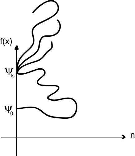
Figure 1. A formal global branching $n$-diagram.

Therefore, according to this, we believe that there is no bifurcation from the branch of trivial solutions at any value of the parameter $n>0$. However, a rigorous proof of this fact is difficult, since our nonlinear operators are not monotone and, hence, the main techniques usually used in the analysis of second-order operators are not applicable here. However, if that was the situation, we could obtain the existence of certain turning points, or even a connection with another branch among the ones emanating from some other eigenfunction $\psi_{k}$, with $k\geq 1$; cf. Figure 1. We plan to carry out this work in a subsequent paper.

5. Blow-up similarity profiles for the Cauchy problem via $n$-branching

5.1. Preliminaries: homotopy and nodal sets

In this section, we describe the behaviour of the blow-up similarity solutions $\eqref{upm}_{-}$ of the TFE-4 (1.1) through the same homotopic approach by setting $n\downarrow 0$ in $\eqref{eigpm}_{-}$ and, hence, arriving at the linear adjoint operator (1.28). Then, we shall use the eigenfunction patterns occurring for $n=0$ (those are generalized Hermite polynomials (3.17)) as branching points for nonlinear eigenfunctions providing us with a straightforward and practical $n$-continuity approach to the self-similar equation (2.8) associated with the TFE-4 (1.1) from the equation (1.11) associated with the bi-harmonic equation (1.8).

It is worth recalling now that homotopic approaches are well-known in the theory of vector fields and nonlinear operator theory (see [16, 31] for details). In our case, a “homotopic path” just declares the existence of a continuous connection (a curve) of some nonlinear eigenfunctions $f=f_{k}^{-}(y)$ satisfying (2.8) that ends up at $n=0^{+}$ at the linear adjoint polynomials $\psi_{k}^{*}(y)$ given in (3.17). Due to Section 3, we already know that those profiles correspond to generalized Hermite polynomials given by (3.17), which have finite oscillatory properties. For instance, for any even $|\beta|$, the polynomials (3.17) do not have any zero nodal surface at all. However, for $k\geq 1$, linear combinations of such eigenfunctions do have nodal sets of known and relatively simple structure.

For odd $|\beta|$ (or on multi-dimensional eigenspaces), arbitrary linear combinations of Hermite polynomials for such a fixed $k=|\beta|\geq 1$ explain all possible structures of nodal sets and (see [26] for a full formulation)

(5.1) multiple zeros of solutions of the bi-harmonic equation (1.8).

Furthermore, it turns out that, using classical branching theory, “nonlinear eigenfunctions” $f_{k}(y)$ of changing sign, which satisfies the nonlinear eigenvalue problem (2.8) (with an extra “radiation-minimal-like” condition at infinity to be specified shortly), at least, for sufficiently small $n>0$, can be connected with the adjoint polynomials $\psi^{*}_{k}(y)$ in (3.17), or their linear combinations from the eigenspace. We are capable of justify this through the corresponding Lyapunov–Schmidt branching equation, trying to be as rigorous as possible in supporting and deriving the critical nonlinear eigenvalues $\alpha_{k}(n)$.

5.2. Towards “minimal growth at infinity”

This is about the “minimal” (a “radiation-like”) condition at infinity, announced in (1.5), which makes the equation (2.8) to be a nonlinear eigenvalue problem. We recall that, for $n=0$, the ${\bf(NEP)_{-}}$ in (1.3) reduces to the linear one for the operator ${\bf B}^{*}$ in (1.28), with the straightforward correspondence

(5.2) $$\textstyle{\alpha_{k}(0)=\lambda_{k}\equiv-\frac{k}{4},\quad k=0,1,2,...\,.}$$

Equation (2.8) admits two kinds of asymptotics at infinity. The first one is nonlinear and is given by the first two operators: assuming simple radial behaviour ($f=y^{\gamma}$) yields

(5.3) $$\textstyle{-\nabla\cdot(|f|^{n}\nabla\Delta f)-\frac{1-\alpha n}{4}\,y\cdot\nabla f+...=0\quad\Longrightarrow\quad f(y)\sim|y|^{\frac{4}{n}}\quad\mbox{as}\quad y\to\infty.}$$

Note that, as $n\to 0^{+}$, precisely this behaviour leads to an exponentially growing bundle, which is prohibited in Theorem 3.2 by specifying the proper weighted space $L^{2}_{\rho^{*}}(\mathbb{R}^{N})$ and eventually leading to the polynomial eigenfunctions (3.17).

The second asymptotics is linear: as $y\to\infty$,

(5.4) $$\textstyle{-\frac{1-\alpha n}{4}\,y\cdot\nabla f-\alpha f+...=0\quad\Longrightarrow\quad f(y)\sim|y|^{\gamma},\quad\mbox{where}\quad\gamma=-\frac{4\alpha}{1-\alpha n}>0,}$$

since by (5.2) we have to assume that $\alpha_{k}(n)<0$ (the first eigenvalue $\alpha_{0}(n)=0$ is not of particular interest; see below) and always $\alpha_{k}(n)<\frac{1}{n}$. Note that then

(5.5) $$\textstyle{\gamma\equiv\frac{4|\alpha|}{1+|\alpha|n}<\frac{4}{n},}$$

so that the linear behaviour (5.4) is the actual minimal one in comparison with (5.3).

Overall, this allows to formulate such a “radiation-like” condition at infinity, which now takes a clear “minimal nature”:

(5.6) find solutions $$f(y)$$ of (2.8) bounded at infinity by functions as in (5.4).

In self-similar approaches and ODE theory, such conditions are known to define similarity solutions of the second kind, a term, which was introduced by Ya.B. Zel’dovich in 1956 [39]. Many of such ODE problems (but indeed, easier) have been rigorously solved since then. For quasilinear elliptic equations such as (2.8), the condition (5.6) is more subtle and delicate indeed. We cannot somehow rigorously justify that the problem (2.8), (5.6) is well posed and admits a countable family of solutions and nonlinear eigenvalues $\{\alpha_{\beta}(n)\}$. We recall that using the homotopy deformation as $n\to 0^{+}$ was our original intention in order to avoid such a difficult “direct” mathematical attack of this nonlinear blow-up eigenvalue problem.

We begin our actual study by noting that the first nonlinear pair for (2.8), (5.6) is trivial: for any $n>0$,

(5.7) $$\alpha_{0}(n)=0\quad\mbox{and}\quad f^{-}_{0}(y)\equiv 1,$$

so that this well corresponds to the first Hermite polynomial from (3.17) with $|\beta|=0$, where $\psi_{0}^{*}(y)\equiv 1$. However, similarity solutions (2.7) with the first eigenfunction in (5.7) are trivial and do not change sign, so, to understand formation of nonlinear “multiple zeros”, we will study branching of eigenfunctions $f_{k}^{-}(y)$ for $k\geq 1$.

5.3. Technical bifurcation calculus

Thus, the critical values $\alpha_{k}(n)$ are obtained for small $n>0$ according to spectral theory established in Section 3. As was noticed, the explicit expression for the eigenvalues and eigenfunctions for the operator ${\bf B}^{*}$ in (1.28) are known; see Theorem 3.2. Moreover, supposing the corresponding linear counterpart from (3.17) with $n=0$, we find, at least formally, that

(5.8) $$\textstyle{\mathcal{L}(\alpha)f:=-\Delta^{2}f-\frac{1}{4}\,y\cdot\nabla f-\alpha f=0.}$$

This equation can be considered as a linear perturbation in terms of the parameter $\alpha$ of that for the adjoint operator ${\bf B}^{*}$ in (1.28). From that equation combined with the eigenvalue expressions obtained for the operator ${\bf B}^{*}$, we derive the critical values for the parameter $\alpha$ given in (5.2), where $\lambda_{k}$ are the eigenvalues defined in Theorem 3.2. Note that those eigenvalues coincide with the eigenvalues of the operator ${\bf B}$. In particular, when $k=0$, we have that $\alpha_{0}=0=\lambda_{0}$ and the eigenfunction is $\psi_{0}^{*}=1$, satisfying

$${\bf B}^{*}\psi_{0}^{*}=0,\quad\mbox{so that}\quad\ker\mathcal{L}(\alpha_{0})=\mathrm{span\,}\{\psi_{0}^{*}=1\}.$$

Hence, $\lambda_{0}=0$ is a simple eigenvalue for the operator $\mathcal{L}(\alpha_{0})={\bf B}^{*}$ and its algebraic multiplicity is 1. In general, we find that (note that $k=0$ is trivial)

(5.9) $$\textstyle{\ker\big{(}{\bf B}^{*}+\frac{k}{4}\,I\big{)}=\mathrm{span\,}\{\psi_{\beta},\,|\beta|=k\},\quad\hbox{for any}\quad k=0,1,2,3,\dots\,,}$$

where the operator ${\bf B}^{*}+\frac{k}{4}\,I$ is Fredholm of index zero. In other words, $R[\mathcal{L}(\alpha_{k})]$ is a closed subspace of $L_{\rho}^{2}(\mathbb{R}^{N})$ and

$$\hbox{dim}\ker(\mathcal{L}(\alpha_{k}))<\infty,\quad\hbox{codim}\,R[\mathcal{L}(\alpha_{k})]<\infty$$

for each $\alpha_{k}$. Moreover, $\dim\ker\big{(}{\bf B}+\frac{k}{4}\,I\big{)}=M_{k}^{*}\geq 1$, for any $k=0,1,2,3,\dots$.

Then, once the relation between (5.8) and the linear operator ${\bf B}^{*}$ has been established, for which we know its spectral theory, by regularity issues in Section 1.4, we can assume for small $n>0$ in (3.17) the following expansions:

(5.10) $$\alpha_{k}(n):=\alpha_{k}+\mu_{1,k}n+o(n),\quad|f|^{n}\equiv|f|^{n}={\mathrm{e}}^{n\ln|f|}:=1+n\ln|f|+o(n),$$

where the last one is assumed to be understood in a weak sense. Again, it is convenient to discuss further the last one. Indeed, the second expansion cannot be interpreted pointwise for oscillatory changing sign solutions $f(y)$, though now these functions are assumed to have finite number of zero surfaces (as the generalized Hermite polynomials for $n=0$ do). However, as usual, this, of course, imposes some restrictions on the possible zeros of the eigenfunctions $\psi_{\beta}^{*}(y)$. According to the spectral theory in Section 3 we already know that those eigenfunctions and their linear combinations for the adjoint operator ${\bf B}^{*}$ are generalized Hermite polynomials given by (3.17). Hence, they are analytic functions with isolated zeros.

Since the possible zeros are isolated, they can be localized in arbitrarily small neighbourhoods. Indeed, it is clear that when $|f|>\delta>0$ for any $\delta>0$, there is no problem in approximating of $|f|^{n}$ as in (5.10), i.e., $|f|^{n}=O(n)$ as $n\rightarrow 0^{+}$. However, when $|f|\leq\delta$ for $\delta\geq 0$ sufficiently small, the proof of such an approximation is far from clear unless the zeros of the $f$’s are all transversal in a natural sense. In view of the expected finite oscillatory nature of solutions $f^{-}(y)$, this should allow one to obtain a weak convergence as in (1.21) to be used in the integral equation similar to (1.18) (with ${\bf B}$ replaced by ${\bf B}^{*}$).

However, let us stress again that, in the present “blow-up” case, we do not need such subtle oscillatory properties of solutions close to interfaces, which are not known in complicated geometries. The point is that, due to the condition (5.6), we are looking for solutions $f(y)$ exhibiting finite oscillatory and sign changing properties, which are similar to those for linear combinations of Hermite polynomials (3.17). Hence, we can suppose that their zeros (zero surfaces) are transversal a.e., so we find that, for $n>0$ and any $\delta=\delta(n)>0$ sufficiently small,

$$n|\ln|f||\gg 1,\quad\hbox{if}\quad|f|\leq\delta(n),$$

and, hence, on such subsets, $f(y)$ must be exponentially small:

$$\textstyle{|\ln|f||\gg\frac{1}{n}\;\Longrightarrow\;\ln|f|\ll-\frac{1}{n}\;\Longrightarrow\;|f|\ll{\mathrm{e}}^{-\frac{1}{n}}.}$$

Thus, we can control the singular coefficients in (5.10), and, in particular, see that

(5.11) $$\ln|f|\in L^{1}_{\rm loc}(\mathbb{R}^{N}).$$

Recall that this happens also in exponentially small neighbourhoods of the transversal zeros.

It is worth recalling again that our computations below are to be understood as those dealing with the equivalent integral equation similar to (1.18) and operators, so, in particular, we can use the powerful facts on compactness of the resolvent $({\bf B}-\lambda I)^{-1}$ and the adjoint one $({\bf B}^{*}-\lambda I)^{-1}$ in the corresponding weighted $L^{2}$-spaces.

Note that, in such an equivalent integral representation, the singular term in (5.10) satisfying (5.11) makes no principal difficulty, so the last expansion in (5.10) makes rather usual sense for applying standard nonlinear operator theory. Overall, the above analysis somehow justifies further branching study. We must admit that this is not a rigorous one, but is indeed sufficient for our formal expansions as $n\to 0^{+}$.

Thus, substituting (5.10) into the nonlinear eigenvalue problem (2.8) and omitting $o(n)$ terms when necessary, we obtain the following expression:

$$\textstyle{-\nabla\cdot[(1+n\ln|f|)\nabla\Delta f]-\frac{1-\alpha_{k}n-\mu_{1,k}n^{2}}{4}\,y\cdot\nabla f-(\alpha_{k}+\mu_{1,k}n)f=0\,,}$$

for any $k=0,1,2,3,\dots$ . Hence, rearranging terms yields

$$\textstyle{-\Delta^{2}f-n\nabla\cdot(\ln|f|\nabla\Delta f)-\frac{1}{4}\,y\cdot\nabla f+\frac{\alpha_{k}n+\mu_{1,k}n^{2}}{4}\,y\cdot\nabla f-\alpha_{k}f-\mu_{1,k}nf=0\,.}$$

In addition, using the expression of the operator ${\bf B}^{*}$ yields

(5.12) $$\textstyle{\big{(}{\bf B}^{*}+\frac{k}{4}\,I\big{)}f+n\mathcal{N}_{k}(f)+o(n)=0\,,}$$

with the operator

(5.13) $$\textstyle{\mathcal{N}_{k}(f):=-\nabla\cdot(\ln|f|\nabla\Delta f)+\frac{\alpha_{k}}{4}\,y\cdot\nabla f-\mu_{1,k}f\,.}$$

Subsequently, we shall compute the coefficients involved in the expansions (5.10) applying the classical Lyapunov–Schmidt method to (5.12) (branching approach when $n\downarrow 0$), and, hence, describing the behaviour of the blow-up solutions for at least small values of the parameter $n>0$. Two cases are distinguished. The first one in which the eigenvalue is simple and the second for which the eigenvalues are semisimple. Note that due to Theorems 3.1 and 3.2, for any $k\geq 0$, the algebraic multiplicities are equal to the geometric ones, so we do not deal with the problem of introducing the generalized eigenfunctions (no Jordan blocks are necessary for restrictions to eigenspaces).

5.4. Simple eigenvalue

Recall that this always happens for $k=0$ (not interesting) and also in 1D and radial geometry, when all the eigenvalues of such ordinary differential operators are simple.

As a typical example, we perform the analysis as for $k=0$, bearing in mind the above other more interesting applications.

Thus, since the first eigenvalue $\lambda_{0}=0$ of ${\bf B}^{*}$ is simple, the dimension of the eigenspace is $M_{0}^{*}=1$, the analysis of this particular case presents less difficulties than the corresponding ones for any other $k\geq 1$. Hence, denoting $\ker\,{\bf B}^{*}=\mathrm{span\,}\{\psi_{0}^{*}=1\}$ and by $Y_{0}^{*}$ the complementary invariant subspace, orthogonal to $\psi_{0}$, we set

(5.14) $$f=\psi_{0}^{*}+V_{0}^{*},$$

where $V_{0}^{*}\in Y_{0}^{*}$. We define $P_{0}^{*}$ and $P_{1}^{*}$ such that $P_{0}^{*}+P_{1}^{*}=I$, to be the projections onto $\ker\,{\bf B}^{*}$ and $Y_{0}^{*}$ respectively. We next set

(5.15) $$V_{0}^{*}:=n\Phi_{1,0}^{*}+o(n).$$

Then, after substituting (5.14) into (5.12) and passing to the limit as $n\rightarrow 0^{+}$, we arrive at a linear inhomogeneous equation for $\Phi_{1,0}^{*}$

(5.16) $${\bf B}^{*}\Phi_{1,0}^{*}=-\mathcal{N}_{0}(\psi_{0}^{*}),$$

since ${\bf B}^{*}\psi_{0}^{*}=0$. By Fredholm’s theory [16] (spectral theory of the pair $\{{\bf B},{\bf B}^{*}\}$ from Section 3 does also matter), a unique solution $V_{0}^{*}\in Y_{0}^{*}$ of (5.16) exists if and only if the right-hand side is orthogonal to the one dimensional kernel of the adjoint operator, in this case ${\bf B}$. In other words, in the topology of the dual space $L^{2}$, the following holds:

(5.17) $$\big{\langle}\mathcal{N}_{0}(\psi_{0}^{*}),\psi_{0}\big{\rangle}=0.$$

Therefore, (5.16) has a unique solution $\Phi_{1,0}^{*}\in Y_{0}^{*}$ determining by (5.15) a bifurcation branch for small $n>0$. In addition, we obtain the following explicit expression for the coefficient $\mu_{1,0}$ of the corresponding nonlinear eigenvalue $\alpha_{0}(n)$ denoted by (5.10):

$$\mu_{1,0}:=\textstyle{\frac{\langle\nabla\cdot(\ln|\psi_{0}^{*}|\nabla\Delta\psi_{0}^{*}),\psi_{0}\rangle}{\langle\psi_{0}^{*},\psi_{0}\rangle}}=\textstyle{\langle\nabla\cdot(\ln|\psi_{0}^{*}|\nabla\Delta\psi_{0}^{*}),\psi_{0}\rangle.}$$

5.5. Multiple eigenvalues for ${\bf k\geq 1}$

For any $k\geq 1$, we know that

$$\textstyle{\dim\ker\big{(}{\bf B}^{*}+\frac{k}{4}\,I\big{)}=M_{k}^{*}>1\quad(\mbox{actually},\,\,\,M_{k}^{*}=M_{k}).}$$

Hence, we have to take the representation

(5.18) $$\textstyle{f=\sum_{|\beta|=k}c_{\beta}\hat{\psi}_{\beta}^{*}+V_{k}^{*},}$$

for every $k\geq 1$. Currently, for convenience, we denote $\{\hat{\psi}_{\beta}^{*}\}_{|\beta|=k}=\{\hat{\psi}_{1}^{*},...,\hat{\psi}_{M_{k}}^{*}\}$, the natural basis of the $M_{k}^{*}$-dimensional eigenspace $\ker\big{(}{\bf B}^{*}+\frac{k}{4}\,I\big{)}$ and set $\psi_{k}^{*}=\sum_{|\beta|=k}c_{\beta}\hat{\psi}_{\beta}^{*}$. Moreover, $V_{k}^{*}\in Y_{k}^{*}$ and $V_{k}^{*}=\sum_{|\beta|>k}c_{\beta}{\psi}_{\beta}^{*}$, where $Y_{k}^{*}$ is the complementary invariant subspace of $\ker\big{(}{\bf B}^{*}+\frac{k}{4}\,I\big{)}$. Furthermore, in the same way as we did for the case $k=0$, we define the $P_{0,k}^{*}$ and $P_{1,k}^{*}$, for every $k\geq 1$, to be the projections of $\ker\big{(}{\bf B}^{*}+\frac{k}{4}\,I\big{)}$ and $Y_{k}^{*}$ respectively. We also denote $V_{k}^{*}$ by

(5.19) $$V_{k}^{*}:=n\Phi_{1,k}^{*}+o(n).$$

Subsequently, substituting (5.18) into (5.12) and passing to the limit as $n\downarrow 0^{+}$, we obtain the following equation:

(5.20) $$\textstyle{\big{(}{\bf B}^{*}+\frac{k}{4}\,I\big{)}\Phi_{1,k}=-\mathcal{N}_{k}\big{(}\sum_{|\beta|=k}c_{\beta}{\psi}_{\beta}^{*}\big{)},}$$

under the natural “normalizing” constraint

(5.21) $$\textstyle{\sum\limits_{|\beta|=k}c_{\beta}=1.}$$

Therefore, applying the Fredholm alternative [16], a unique $V_{k}^{*}\in Y_{k}^{*}$ exists if and only if the right-hand side of (5.20) is orthogonal to $\ker\,\big{(}{\bf B}^{*}+\frac{k}{4}\,I\big{)}$. Multiplying the right-hand side of (5.20) by $\psi_{\beta}$, for every $|\beta|$, in the topology of the dual space $L^{2}$, we obtain an algebraic system of $M_{k}^{*}+1$ equations and the same number of unknowns, $\{c_{\beta},\,|\beta|=k\}$ and $\mu_{1,k}$:

(5.22) $$\textstyle{\big{\langle}\mathcal{N}_{k}(\sum_{|\beta|=k}c_{\beta}{\psi}_{\beta}^{*}),\psi_{\beta}\big{\rangle}=0\quad\mbox{for all}\quad|\beta|=k,}$$

which is indeed the Lyapunov–Schmidt branching equation [38]. Through that algebraic system we shall ascertain the coefficients of the expansions (5.10) and, hence, eventually the directions of branching, as well as the number of branches. However, a full solution of the non-variational algebraic system (5.22) is a very difficult issue, though we claim that the number of branches is expected to be related to the dimension of the eigenspace $\ker\,\big{(}{\bf B}^{*}+\frac{k}{4}\,I\big{)}$.

In order to obtain the number of possible branches and with the objective of avoiding excessive notation, we analyze two typical cases.

Computations for branching of dipole solutions in 2D. Firstly, we ascertain some expressions for those coefficients in the case when $|\beta|=1$, $N=2$ and $M_{1}^{*}=2$, so that, in our notations, $\{\psi_{\beta}\}_{|\beta|=1}=\{\hat{\psi}_{1}^{*},\hat{\psi}_{2}^{*}\}$ such that $\psi_{1}^{*}=c_{1}\hat{\psi}_{1}^{*}+c_{2}\hat{\psi}_{2}^{*}$. Consequently, in this case, we obtain the following algebraic system:

(5.23) $$\left\{\begin{array}[]{l}c_{1}\langle\hat{\psi}_{1},h_{1}\rangle+\frac{c_{1}\alpha_{1}}{4}\,\langle\hat{\psi}_{1},y\cdot\nabla\hat{\psi}_{1}^{*}\rangle-c_{1}\mu_{1,1}+c_{2}\langle\hat{\psi}_{1},h_{2}\rangle+\frac{c_{2}\alpha_{1}}{4}\,\langle\hat{\psi}_{1},y\cdot\nabla\hat{\psi}_{2}^{*}\rangle=0,\vskip 3.0pt plus 1.0pt minus 1.0pt\\ c_{1}\langle\hat{\psi}_{2},h_{1}\rangle+\frac{c_{1}\alpha_{1}}{4}\,\langle\hat{\psi}_{2},y\cdot\nabla\hat{\psi}_{1}^{*}\rangle+c_{2}\langle\hat{\psi}_{2},h_{2}\rangle+\frac{c_{2}\alpha_{1}}{4}\,\langle\hat{\psi}_{2},y\cdot\nabla\hat{\psi}_{2}^{*}\rangle-c_{2}\mu_{1,1}=0,\vskip 3.0pt plus 1.0pt minus 1.0pt\\ c_{1}+c_{2}=1,\end{array}\right.$$

where

$$h_{1}:=-\nabla\cdot[\ln(c_{1}\hat{\psi}_{1}^{*}+c_{2}\hat{\psi}_{2}^{*})\nabla\Delta\hat{\psi}_{1}^{*}],\,\,h_{2}:=-\nabla\cdot[\ln(c_{1}\hat{\psi}_{1}^{*}+c_{2}\hat{\psi}_{2}^{*})\nabla\Delta\hat{\psi}_{2}^{*}],$$

and, $c_{1}$, $c_{2}$ and $\mu_{1,1}$ are the coefficients that we want to calculate. Also, $\alpha_{1}=\lambda_{1}$ is regarded as the value of the parameter $\alpha$ denoted by (5.2) such that $\hat{\psi}_{1,2}^{*}$ are the corresponding associated adjoint eigenfunctions. Now, from the third equation we have $c_{2}=1-c_{1}$, so that substituting it into the first two equations of (4.5) gives

(5.24) $$\left\{\begin{array}[]{l}0=N_{1}(c_{1},\mu_{1,1})+c_{1}\frac{\alpha_{1}}{4}\,\big{[}\langle\hat{\psi}_{1},y\cdot\nabla\hat{\psi}_{1}^{*}\rangle-\langle\hat{\psi}_{1},y\cdot\nabla\hat{\psi}_{2}^{*}\rangle\big{]},\vskip 3.0pt plus 1.0pt minus 1.0pt\\ 0=N_{2}(c_{1},\mu_{1,1})+c_{1}\frac{\alpha_{1}}{4}\,\big{[}\langle\hat{\psi}_{2},y\cdot\nabla\hat{\psi}_{1}^{*}\rangle-\langle\hat{\psi}_{2},y\cdot\nabla\hat{\psi}_{2}^{*}\rangle\big{]}-\mu_{1,1},\end{array}\right.$$

where

$$\begin{split}&\textstyle{N_{1}(c_{1},\mu_{1,1}):=c_{1}\langle\hat{\psi}_{1},h_{1}\rangle+\langle\hat{\psi}_{1},h_{2}\rangle+\frac{\alpha_{1}}{4}\,\langle\hat{\psi}_{1},y\cdot\nabla\hat{\psi}_{2}^{*}\rangle-c_{1}\langle\hat{\psi}_{1},h_{2}\rangle-c_{1}\mu_{1,1},}\\ &\textstyle{N_{2}(c_{1},\mu_{1,1}):=c_{1}\langle\hat{\psi}_{2},h_{1}\rangle+\langle\hat{\psi}_{2},h_{2}\rangle+\frac{\alpha_{1}}{4}\,\langle\hat{\psi}_{2},y\cdot\nabla\hat{\psi}_{2}^{*}\rangle-c_{1}\langle\hat{\psi}_{2},h_{2}\rangle+c_{1}\mu_{1,1}}\end{split}$$

represent the nonlinear parts of the algebraic system, with $h_{0}$ and $h_{1}$ just depending on $c_{1}$ in this case.

To detect solutions for the system (5.23) we apply the Brouwer fixed point theorem to (5.24) (see [1] for further details). Then, we suppose that the values $c_{1}$ and $\mu_{1,1}$ are the unknowns in a sufficiently big disc $D_{R}(\hat{c}_{1},\hat{\mu}_{1,1})$, centered in a possible nondegenerate zero $(\hat{c}_{1},\hat{\mu}_{1,1})$. Therefore, if one of the next two conditions are satisfied

$$\langle\hat{\psi}_{1},y\cdot\nabla\hat{\psi}_{1}^{*}\rangle-\langle\hat{\psi}_{1},y\cdot\nabla\hat{\psi}_{2}^{*}\rangle\neq 0\quad\hbox{or}\quad\langle\hat{\psi}_{2},y\cdot\nabla\hat{\psi}_{2}^{*}\rangle-\langle\hat{\psi}_{2},y\cdot\nabla\hat{\psi}_{1}^{*}\rangle\neq 0,$$

the nonlinear algebraic system (5.24) has at least one non-degenerate solution. Note that multiplicity results are extremely difficult to obtain. So, to ascertain the number of solutions for those nonlinear finite-dimensional algebraic problems is rather complicated. However, we expect, and in fact compute it in some cases, that this is somehow related to the dimension of the corresponding eigenspace $\ker\,\big{(}{\bf B}^{*}+\frac{k}{4}\,I\big{)}$, $k\geq 1$.

Firstly, we calculate the number of solutions for the nonlinear algebraic system (5.23). Integrating by parts the terms in which $h_{1}$ and $h_{2}$ are involved in the first two equations and rearranging terms, we arrive at (as usual, all integrals are over $\mathbb{R}^{N}$)

$$\textstyle{\int\nabla\psi_{1}\cdot\ln(c_{1}\hat{\psi}_{1}^{*}+c_{2}\hat{\psi}_{2}^{*})\nabla\Delta(c_{1}\hat{\psi}_{1}^{*}+c_{2}\hat{\psi}_{2}^{*})} \textstyle{+c_{1}\frac{\alpha_{1}}{4}\,\int\hat{\psi}_{1}y\cdot\nabla\hat{\psi}_{1}^{*}-c_{1}\mu_{1,1}}$$

$$\textstyle{+c_{2}\frac{\alpha_{1}}{4}\,\int\hat{\psi}_{1}y\cdot\nabla\hat{\psi}_{2}^{*}=0,}$$

$$\textstyle{\int\nabla\hat{\psi}_{2}\cdot\ln(c_{1}\hat{\psi}_{1}^{*}+c_{2}\hat{\psi}_{2}^{*})\nabla\Delta(c_{2}\hat{\psi}_{1}^{*}+c_{2}\hat{\psi}_{2}^{*})} \textstyle{+c_{1}\frac{\alpha_{1}}{4}\,\int\hat{\psi}_{2}y\cdot\nabla\hat{\psi}_{1}^{*}-c_{2}\mu_{1,1}}$$

$$\textstyle{+c_{2}\frac{\alpha_{1}}{4}\,\int\hat{\psi}_{2}y\cdot\nabla\hat{\psi}_{2}^{*}=0.}$$

Then, substituting the third equation with the expression $c_{1}=1-c_{2}$ and, hence, putting $c_{1}\hat{\psi}_{1}^{*}+c_{2}\hat{\psi}_{2}^{*}=\hat{\psi}_{1}^{*}+(\hat{\psi}_{2}^{*}-\hat{\psi}_{1}^{*})c_{2}$ into those two equations obtained above yields

$$\textstyle{\int\nabla\hat{\psi}_{1}\cdot\ln(\hat{\psi}_{1}^{*}+} \textstyle{(\hat{\psi}_{2}^{*}-\hat{\psi}_{1}^{*})c_{2})\nabla\Delta(\hat{\psi}_{1}^{*}+(\hat{\psi}_{2}^{*}-\hat{\psi}_{1}^{*})c_{2})-\mu_{1,1}+c_{2}\mu_{1,1}}$$

$$\textstyle{+\frac{\alpha_{1}}{4}\,\int\hat{\psi}_{1}y\cdot\nabla\hat{\psi}_{1}^{*}+c_{2}\frac{\alpha_{1}}{4}\,\int\hat{\psi}_{1}y\cdot(\nabla\hat{\psi}_{2}^{*}-\nabla\hat{\psi}_{1}^{*})=0,}$$

(5.25) $$\begin{split}\textstyle{\int\nabla\hat{\psi}_{2}\cdot\ln(\hat{\psi}_{1}^{*}+}&\textstyle{(\hat{\psi}_{2}^{*}-\hat{\psi}_{1}^{*})c_{2})\nabla\Delta(\hat{\psi}_{1}^{*}+(\hat{\psi}_{2}^{*}-\hat{\psi}_{1}^{*})c_{2})-c_{2}\mu_{1,1}}\\ &\textstyle{+\frac{\alpha_{1}}{4}\,\int\hat{\psi}_{2}y\cdot\nabla\hat{\psi}_{1}^{*}+c_{2}\frac{\alpha_{1}}{4}\,\int\hat{\psi}_{2}y\cdot(\nabla\hat{\psi}_{2}^{*}-\nabla\hat{\psi}_{1}^{*})=0.}\end{split}$$

Subsequently, adding both equations, we have that

$$\mu_{1,1} =\textstyle{\int(\nabla\hat{\psi}_{1}+\nabla\hat{\psi}_{2})\cdot\ln(\hat{\psi}_{1}^{*}+(\hat{\psi}_{2}^{*}-\hat{\psi}_{1}^{*})c_{2})\nabla\Delta(\hat{\psi}_{1}^{*}+(\hat{\psi}_{2}^{*}-\hat{\psi}_{1}^{*})c_{2})}$$

$$\textstyle{+\frac{\alpha_{1}}{4}\,\int(\hat{\psi}_{1}+\hat{\psi}_{2})y\cdot\nabla\hat{\psi}_{1}^{*}+c_{2}\frac{\alpha_{1}}{4}\,\int(\hat{\psi}_{1}+\hat{\psi}_{2})y\cdot(\nabla\hat{\psi}_{2}^{*}-\nabla\hat{\psi}_{1}^{*}).}$$

Substituting it into the second equation of (5.25), we find the following equation with the single unknown $c_{2}$:

(5.26) $$\begin{split}&\textstyle{-c_{2}^{2}\frac{\alpha_{1}}{4}\,\int(\hat{\psi}_{1}+\hat{\psi}_{2})y\cdot(\nabla\hat{\psi}_{2}^{*}-\nabla\hat{\psi}_{1}^{*})+c_{2}\frac{\alpha_{1}}{4}(\,\int\hat{\psi}_{2}y\cdot\nabla\hat{\psi}_{2}^{*}-\,\int(\hat{\psi}_{1}+2\hat{\psi}_{2})y\cdot\nabla\hat{\psi}_{1}^{*})}\\ &\textstyle{+\frac{\alpha_{1}}{4}\,\int\hat{\psi}_{2}y\cdot\nabla\hat{\psi}_{1}^{*}+\int\nabla\hat{\psi}_{2}\cdot\ln(\hat{\psi}_{1}^{*}+(\hat{\psi}_{2}^{*}-\hat{\psi}_{1}^{*})c_{2})\nabla\Delta(\hat{\psi}_{1}^{*}+(\hat{\psi}_{2}^{*}-\hat{\psi}_{1}^{*})c_{2})}\\ &\textstyle{-c_{2}\int(\nabla\hat{\psi}_{1}+\nabla\hat{\psi}_{2})\cdot\ln(\hat{\psi}_{1}^{*}+(\hat{\psi}_{2}^{*}-\hat{\psi}_{1}^{*})c_{2})\nabla\Delta(\hat{\psi}_{1}^{*}+(\hat{\psi}_{2}^{*}-\hat{\psi}_{1}^{*})c_{2})=0,}\end{split}$$

which can be written in the following way:

(5.27) $$c_{2}^{2}A+c_{2}B+C+\omega(c_{2})\equiv\mathfrak{F}(c_{2})+\omega(c_{2})=0.$$

Here $\omega(c_{2})$ can be considered as a perturbation of the quadratic form $\mathfrak{F}(c_{2})$ with the coefficients of such a quadratic form defined by

$$\textstyle{A:=-\frac{\alpha_{1}}{4}\,\int(\hat{\psi}_{1}+\hat{\psi}_{2})y\cdot(\nabla\hat{\psi}_{2}^{*}-\nabla\hat{\psi}_{1}^{*}),}$$

$$\textstyle{B:=\frac{\alpha_{1}}{4}(\,\int\hat{\psi}_{2}y\cdot\nabla\nabla\hat{\psi}_{2}^{*}-\,\int(\hat{\psi}_{1}+2\hat{\psi}_{2})y\cdot\nabla\hat{\psi}_{1}^{*}),}$$

$$C:=\textstyle{\frac{\alpha_{1}}{4}\,\int\hat{\psi}_{2}y\cdot\nabla\hat{\psi}_{1}^{*},}$$

$$\omega(c_{2}):=\textstyle{\int\nabla\hat{\psi}_{2}\cdot\ln(\hat{\psi}_{1}^{*}+(\hat{\psi}_{2}^{*}-\hat{\psi}_{1}^{*})c_{2})\nabla\Delta(\hat{\psi}_{1}^{*}+(\hat{\psi}_{2}^{*}-\hat{\psi}_{1}^{*})c_{2})}$$

$$\textstyle{-c_{2}\int(\nabla\hat{\psi}_{1}+\nabla\hat{\psi}_{2})\cdot\ln(\hat{\psi}_{1}^{*}+(\hat{\psi}_{2}^{*}-\hat{\psi}_{1}^{*})c_{2})\nabla\Delta(\hat{\psi}_{1}^{*}+(\hat{\psi}_{2}^{*}-\hat{\psi}_{1}^{*})c_{2}).}$$

Hence, due to the normalizing constraint (5.21), $c_{2}\in[0,1]$, solving the quadratic equation $\mathfrak{F}(c_{2})=0$ yields:

1. $c_{2}=0\Longrightarrow\mathfrak{F}(0)=C$;

2. $c_{2}=1\Longrightarrow\mathfrak{F}(1)=A+B+C$; and

3. differentiating $\mathfrak{F}$ with respect to $c_{2}$, we obtain that $\mathfrak{F}^{\prime}(c_{2})=2c_{2}A+B$. Then, the critical point of the function $\mathfrak{F}$ is $c_{2}^{*}=-\frac{B}{2A}$ and its image is $\mathfrak{F}(c_{2}^{*})=-\frac{B}{4A}+C$.

Therefore, since we know about the existence of at least one solution, different from zero, in this particular case we impose some conditions in order to have at most two solutions:

1. $C(A+B+C)>0$;

2. $C\big{(}-\frac{B}{4A}+C\big{)}<0$; and

3. $0<-\frac{B}{2A}<1$.

Note that, for $-\frac{B}{4A}+C=0$, we have just a single solution.

Consequently, going back again to the equation (5.27), we need to control somehow the perturbation of the quadratic form to maintain the number of solutions. Therefore, controlling the possible oscillations of the perturbation $\omega(c_{2})$ in such a way that

$$\left\|\omega(c_{2})\right\|_{L^{\infty}}\leq\mathfrak{F}(c_{2}^{*}),$$

we can assure that the number of solutions for (5.23) is exactly two (or at most two). This is actually the dimension of the kernel for the operator ${\bf B}+\frac{1}{4}\,I$ as we conjectured. Note that, in general and for large $k\gg 1$, to solve such multiplicity problems for those types of non-variational equations is a rather difficult open problem.

Branching computations for $|\beta|=2$. Subsequently, we shall extend those results for the case in which the dimension of the eigenspace is greater than 1. Again the calculus are rather tedious. For that reason we find it easier to make such calculations for the particular case when $|\beta|=2$ and $M_{2}^{*}=3$ ($N=2$), so that $\{\psi_{\beta}^{*}\}_{|\beta|=2}=\{\hat{\psi}_{1}^{*},\hat{\psi}_{2}^{*},\hat{\psi}_{3}^{*}\}$ stands for a basis of the eigenspace $\ker\big{(}{\bf B}^{*}+\frac{1}{2}\,I\big{)}$, with $k=2$ and $\lambda_{k}=-\frac{k}{4}$ as the associated eigenvalue. Observe that $\alpha_{k}(0)=\lambda_{k}$.

Thus, in this case, performing in a similar way as was done for (5.23) with $\psi_{2}^{*}=c_{1}\hat{\psi}_{1}^{*}+c_{2}\hat{\psi}_{2}^{*}+c_{3}\hat{\psi}_{3}^{*}$, we arrive at the following algebraic system:

(5.28) $$\left\{\begin{array}[]{l}\begin{array}[]{r}c_{1}\langle\hat{\psi}_{1},h_{1}\rangle+c_{2}\langle\hat{\psi}_{1},h_{2}\rangle+c_{3}\langle\hat{\psi}_{1},h_{3}\rangle+\frac{c_{1}\alpha_{2}}{4}\,\langle\hat{\psi}_{1},y\cdot\nabla\hat{\psi}_{1}^{*}\rangle+\frac{c_{2}\alpha_{2}}{4}\,\langle\hat{\psi}_{1},y\cdot\nabla\hat{\psi}_{2}^{*}\rangle\\ +\frac{c_{3}\alpha_{2}}{4}\,\langle\hat{\psi}_{1},y\cdot\nabla\hat{\psi}_{3}^{*}\rangle-c_{1}\mu_{1,2}=0,\vskip 3.0pt plus 1.0pt minus 1.0pt\\ c_{1}\langle\hat{\psi}_{2},h_{1}\rangle+c_{2}\langle\hat{\psi}_{2},h_{2}\rangle+c_{2}\langle\hat{\psi}_{2},h_{3}\rangle+\frac{c_{1}\alpha_{2}}{4}\,\langle\hat{\psi}_{2},y\cdot\nabla\hat{\psi}_{1}^{*}\rangle+\frac{c_{2}\alpha_{2}}{4}\,\langle\hat{\psi}_{2},y\cdot\nabla\hat{\psi}_{2}^{*}\rangle\\ +\frac{c_{3}\alpha_{2}}{4}\,\langle\hat{\psi}_{2},y\cdot\nabla\hat{\psi}_{3}^{*}\rangle-c_{2}\mu_{1,2}=0,\vskip 3.0pt plus 1.0pt minus 1.0pt\\ c_{1}\langle\hat{\psi}_{3},h_{1}\rangle+c_{2}\langle\hat{\psi}_{3},h_{2}\rangle+c_{2}\langle\hat{\psi}_{3},h_{3}\rangle+\frac{c_{1}\alpha_{2}}{4}\,\langle\hat{\psi}_{3},y\cdot\nabla\hat{\psi}_{1}^{*}\rangle+\frac{c_{2}\alpha_{2}}{4}\,\langle\hat{\psi}_{3},y\cdot\nabla\hat{\psi}_{2}^{*}\rangle\\ +\frac{c_{3}\alpha_{2}}{4}\,\langle\hat{\psi}_{3},y\cdot\nabla\hat{\psi}_{3}^{*}\rangle-c_{3}\mu_{1,2}=0,\end{array}\\ c_{1}+c_{2}+c_{3}=1,\end{array}\right.$$

where

$$h_{1}:=-\nabla\cdot[\ln(c_{1}\hat{\psi}_{1}^{*}+c_{2}\hat{\psi}_{2}^{*}+c_{3}\hat{\psi}_{3}^{*})\nabla\Delta\hat{\psi}_{1}^{*}],\,\,h_{2}:=-\nabla\cdot[\ln(c_{1}\hat{\psi}_{1}^{*}+c_{2}\hat{\psi}_{2}^{*}+c_{3}\hat{\psi}_{3}^{*})\nabla\Delta\hat{\psi}_{2}^{*}],$$

$$\hbox{and}\quad h_{3}:=-\nabla\cdot[\ln(c_{1}\hat{\psi}_{1}^{*}+c_{2}\hat{\psi}_{2}^{*}+c_{3}\hat{\psi}_{3}^{*})\nabla\Delta\hat{\psi}_{3}^{*}],\,\,$$

and $c_{1}$, $c_{2}$, $c_{3}$, and $\mu_{1,2}$ are unknowns. Here, $\hat{\psi}_{1},\hat{\psi}_{2},\hat{\psi}_{3}$ represent the eigenfunctions associated with the eigenvalue $\lambda_{2}=\alpha_{2}(0)$ and $\hat{\psi}_{1}^{*},\hat{\psi}_{2}^{*},\hat{\psi}_{3}^{*}$ are the corresponding adjoint eigenfunctions, which are associated with the same eigenvalue $\lambda_{2}$.

As for the case $|\beta|=1$, the application of the Brouwer fixed point theorem and the topological degree provide us with the existence of a non-degenerate solution for the nonlinear algebraic system (5.28) under certain conditions.

Furthermore, in the subsequent analysis, we shall show a possible way to ascertain the number of solutions of the nonlinear algebraic system (5.28). Obviously, since the dimension of the eigenspace is bigger than the corresponding one in the case $|\beta|=1$, the difficulty in obtaining multiplicity results increases.

We proceed as in the previous case. Firstly, we integrate by parts those terms in which $h_{1}$, $h_{2}$, and $h_{3}$ are involved. After rearranging terms, this yields

$$\textstyle{\int\nabla\psi_{1}\cdot\ln(c_{1}\hat{\psi}_{1}^{*}+c_{2}\hat{\psi}_{2}^{*}+c_{3}\hat{\psi}_{3}^{*})} \textstyle{\nabla\Delta(c_{1}\hat{\psi}_{1}^{*}+c_{2}\hat{\psi}_{2}^{*}+c_{3}\hat{\psi}_{3}^{*})}\textstyle{+c_{1}\frac{\alpha_{2}}{4}\,\int\hat{\psi}_{1}y\cdot\nabla\hat{\psi}_{1}^{*}-c_{1}\mu_{1,2}}$$

$$\textstyle{+c_{2}\frac{\alpha_{2}}{4}\,\int\hat{\psi}_{1}y\cdot\nabla\hat{\psi}_{2}^{*}+c_{3}\frac{\alpha_{2}}{4}\,\int\hat{\psi}_{1}y\cdot\nabla\hat{\psi}_{3}^{*}=0;}$$

$$\textstyle{\int\nabla\hat{\psi}_{2}\cdot\ln(c_{1}\hat{\psi}_{1}^{*}+c_{2}\hat{\psi}_{2}^{*}+c_{3}\hat{\psi}_{3}^{*})} \textstyle{\nabla\Delta(c_{2}\hat{\psi}_{1}^{*}+c_{2}\hat{\psi}_{2}^{*}+c_{3}\hat{\psi}_{3}^{*})}\textstyle{+c_{1}\frac{\alpha_{2}}{4}\,\int\hat{\psi}_{2}y\cdot\nabla\hat{\psi}_{1}^{*}-c_{2}\mu_{1,2}}$$

$$\textstyle{+c_{2}\frac{\alpha_{2}}{4}\,\int\hat{\psi}_{2}y\cdot\nabla\hat{\psi}_{2}^{*}+c_{3}\frac{\alpha_{2}}{4}\,\int\hat{\psi}_{2}y\cdot\nabla\hat{\psi}_{3}^{*}=0;}$$

$$\textstyle{\int\nabla\hat{\psi}_{3}\cdot\ln(c_{1}\hat{\psi}_{1}^{*}+c_{2}\hat{\psi}_{2}^{*}+c_{3}\hat{\psi}_{3}^{*})} \textstyle{\nabla\Delta(c_{2}\hat{\psi}_{1}^{*}+c_{2}\hat{\psi}_{2}^{*}+c_{3}\hat{\psi}_{3}^{*})}\textstyle{+c_{1}\frac{\alpha_{2}}{4}\,\int\hat{\psi}_{3}y\cdot\nabla\hat{\psi}_{1}^{*}-c_{3}\mu_{1,2}}$$

$$\textstyle{+c_{2}\frac{\alpha_{2}}{4}\,\int\hat{\psi}_{3}y\cdot\nabla\hat{\psi}_{2}^{*}+c_{3}\frac{\alpha_{2}}{4}\,\int\hat{\psi}_{3}y\cdot\nabla\hat{\psi}_{3}^{*}=0.}$$

Next, by the fourth equation in (5.28), we have that $c_{1}=1-c_{2}-c_{3}$. Then, setting

$$c_{1}\hat{\psi}_{1}+c_{2}\hat{\psi}_{2}+c_{3}\hat{\psi}_{3}=\hat{\psi}_{1}+c_{2}(\hat{\psi}_{2}-\hat{\psi}_{1})+c_{3}(\hat{\psi}_{3}-\hat{\psi}_{1})$$

and substituting this into three equations above yields a nonlinear algebraic system:

$$\textstyle{\int\nabla\hat{\psi}_{1}\cdot\ln(\hat{\psi}_{1}^{*}+} \textstyle{(\hat{\psi}_{2}^{*}-\hat{\psi}_{1}^{*})c_{2}+(\hat{\psi}_{3}^{*}-\hat{\psi}_{1}^{*})c_{3})\nabla\Delta(\hat{\psi}_{1}^{*}+(\hat{\psi}_{2}^{*}-\hat{\psi}_{1}^{*})c_{2}+(\hat{\psi}_{3}^{*}-\hat{\psi}_{1}^{*})c_{3})}$$

$$\textstyle{-\mu_{1,2}+c_{2}\mu_{1,2}+c_{3}\mu_{1,2}+\frac{\alpha_{2}}{4}\,\int\hat{\psi}_{1}y\cdot\nabla\hat{\psi}_{1}^{*}}$$

$$\textstyle{+\frac{\alpha_{2}}{4}\,\int\hat{\psi}_{1}y\cdot((\nabla\hat{\psi}_{2}^{*}-\nabla\hat{\psi}_{1}^{*})c_{2}+(\nabla\hat{\psi}_{3}^{*}-\nabla\hat{\psi}_{1}^{*})c_{3})=0;}$$

$$\textstyle{\int\nabla\hat{\psi}_{2}\cdot\ln(\hat{\psi}_{1}^{*}+} \textstyle{(\hat{\psi}_{2}^{*}-\hat{\psi}_{1}^{*})c_{2}+(\hat{\psi}_{3}^{*}-\hat{\psi}_{1}^{*})c_{3})\nabla\Delta(\hat{\psi}_{1}^{*}+(\hat{\psi}_{2}^{*}-\hat{\psi}_{1}^{*})c_{2}+(\hat{\psi}_{3}^{*}-\hat{\psi}_{1}^{*})c_{3})}$$

$$\textstyle{-c_{2}\mu_{1,2}+\frac{\alpha_{2}}{4}\,\int\hat{\psi}_{2}y\cdot\nabla\hat{\psi}_{1}^{*}}$$

$$\textstyle{+\frac{\alpha_{2}}{4}\,\int\hat{\psi}_{2}y\cdot((\nabla\hat{\psi}_{2}^{*}-\nabla\hat{\psi}_{1}^{*})c_{2}+(\nabla\hat{\psi}_{3}^{*}-\nabla\hat{\psi}_{1}^{*})c_{3})=0;}$$

(5.29) $$\begin{split}\textstyle{\int\nabla\hat{\psi}_{3}\cdot\ln(\hat{\psi}_{1}^{*}+}&\textstyle{(\hat{\psi}_{2}^{*}-\hat{\psi}_{1}^{*})c_{2}+(\hat{\psi}_{3}^{*}-\hat{\psi}_{1}^{*})c_{3})\nabla\Delta(\hat{\psi}_{1}^{*}+(\hat{\psi}_{2}^{*}-\hat{\psi}_{1}^{*})c_{2}+(\hat{\psi}_{3}^{*}-\hat{\psi}_{1}^{*})c_{3})}\\ &\textstyle{-c_{3}\mu_{1,2}+\frac{\alpha_{2}}{4}\,\int\hat{\psi}_{3}y\cdot\nabla\hat{\psi}_{1}^{*}}\\ &\textstyle{+\frac{\alpha_{2}}{4}\,\int\hat{\psi}_{3}y\cdot((\nabla\hat{\psi}_{2}^{*}-\nabla\hat{\psi}_{1}^{*})c_{2}+(\nabla\hat{\psi}_{3}^{*}-\nabla\hat{\psi}_{1}^{*})c_{3})=0.}\end{split}$$

Now, adding the first equation of (5.29) to the other two ones, we have that

$$\textstyle{\int(\nabla\hat{\psi}_{1}+\nabla\hat{\psi}_{2})\cdot\ln(\hat{\psi}_{1}^{*}+} \textstyle{(\hat{\psi}_{2}^{*}-\hat{\psi}_{1}^{*})c_{2}+(\hat{\psi}_{3}^{*}-\hat{\psi}_{1}^{*})c_{3})\nabla\Delta(\hat{\psi}_{1}^{*}+(\hat{\psi}_{2}^{*}-\hat{\psi}_{1}^{*})c_{2}+(\hat{\psi}_{3}^{*}-\hat{\psi}_{1}^{*})c_{3})}$$

$$\textstyle{-\mu_{1,2}+c_{3}\mu_{1,2}+\frac{\alpha_{2}}{4}\,\int(\hat{\psi}_{1}+\hat{\psi}_{2})y\cdot\nabla\hat{\psi}_{1}^{*}}$$

$$\textstyle{+\frac{\alpha_{2}}{4}\,\int(\hat{\psi}_{1}+\hat{\psi}_{2})y\cdot((\nabla\hat{\psi}_{2}^{*}-\nabla\hat{\psi}_{1}^{*})c_{2}+(\nabla\hat{\psi}_{3}^{*}-\nabla\hat{\psi}_{1}^{*})c_{3})=0,}$$

$$\textstyle{\int(\nabla\hat{\psi}_{1}+\nabla\hat{\psi}_{3})\cdot\ln(\hat{\psi}_{1}^{*}+} \textstyle{(\hat{\psi}_{2}^{*}-\hat{\psi}_{1}^{*})c_{2}+(\hat{\psi}_{3}^{*}-\hat{\psi}_{1}^{*})c_{3})\nabla\Delta(\hat{\psi}_{1}^{*}+(\hat{\psi}_{2}^{*}-\hat{\psi}_{1}^{*})c_{2}+(\hat{\psi}_{3}^{*}-\hat{\psi}_{1}^{*})c_{3})}$$

$$\textstyle{-\mu_{1,2}+c_{2}\mu_{1,2}+\frac{\alpha_{2}}{4}\,\int(\hat{\psi}_{1}+\hat{\psi}_{3})y\cdot\nabla\hat{\psi}_{1}^{*}}$$

$$\textstyle{+\frac{\alpha_{2}}{4}\,\int(\hat{\psi}_{1}+\hat{\psi}_{3})y\cdot((\nabla\hat{\psi}_{2}^{*}-\nabla\hat{\psi}_{1}^{*})c_{2}+(\nabla\hat{\psi}_{3}^{*}-\nabla\hat{\psi}_{1}^{*})c_{3})=0.}$$

Subsequently, subtracting those equations yields

$$\textstyle{\mu_{1,2}} \textstyle{=\frac{1}{c_{2}-c_{3}}\,\big{[}\int(\nabla\hat{\psi}_{2}-\nabla\hat{\psi}_{3})\cdot\ln\Psi^{*}\nabla\Delta\Psi^{*}+\frac{\alpha_{2}}{4}\,\int(\hat{\psi}_{2}-\hat{\psi}_{3})y\cdot\nabla\hat{\psi}_{1}^{*}}$$

$$\textstyle{+\frac{\alpha_{2}}{4}\,\int(\hat{\psi}_{2}-\hat{\psi}_{3})y\cdot((\nabla\hat{\psi}_{2}^{*}-\nabla\hat{\psi}_{1}^{*})c_{2}+(\nabla\hat{\psi}_{3}^{*}-\nabla\hat{\psi}_{1}^{*})c_{3})\big{]},}$$

where $\Psi^{*}=\hat{\psi}_{1}^{*}+(\hat{\psi}_{2}^{*}-\hat{\psi}_{1}^{*})c_{2}+(\hat{\psi}_{3}^{*}-\hat{\psi}_{1}^{*})c_{3}$. Thus, substituting it into (5.29), we arrive at the following system, with $c_{2}$ and $c_{3}$ as the unknowns:

$$\textstyle{c_{3}\int(\nabla\hat{\psi}_{1}-\nabla\hat{\psi}_{2}} \textstyle{+\nabla\hat{\psi}_{3})\cdot\ln\Psi\nabla\Delta\Psi^{*}-c_{2}\int(\nabla\hat{\psi}_{1}+\nabla\hat{\psi}_{2}-\nabla\hat{\psi}_{3})\cdot\ln\Psi\nabla\Delta\Psi^{*}}$$

$$\textstyle{+\int(\nabla\hat{\psi}_{2}-\nabla\hat{\psi}_{3})\cdot\ln\Psi^{*}+\frac{\alpha_{2}}{4}\int(\hat{\psi}_{2}-\hat{\psi}_{3})y\cdot\nabla\hat{\psi}_{1}^{*}\,}$$

$$\textstyle{+c_{2}\frac{\alpha_{2}}{4}\,\big{[}\int(\hat{\psi}_{2}-\hat{\psi}_{3})y\cdot\nabla(\hat{\psi}_{2}^{*}-2\hat{\psi}_{1}^{*})-\int\hat{\psi}_{1}y\cdot\nabla\hat{\psi}_{1}^{*}\big{]}}$$

$$\textstyle{+c_{3}\frac{\alpha_{2}}{4}\,\big{[}\int(\hat{\psi}_{2}-\hat{\psi}_{3})y\cdot\nabla(\hat{\psi}_{3}^{*}-2\hat{\psi}_{1}^{*})-\int\hat{\psi}_{1}y\cdot\nabla\hat{\psi}_{1}^{*}\big{]}}$$

$$\textstyle{+c_{2}c_{3}\frac{\alpha_{2}}{4}\big{[}\,\int\hat{\psi}_{1}y\cdot(\nabla\hat{\psi}_{2}^{*}-\nabla\hat{\psi}_{3}^{*})}$$

$$\textstyle{+\,\int(\hat{\psi}_{2}-\hat{\psi}_{3})y\cdot(2\nabla\hat{\psi}_{1}^{*}-\nabla\hat{\psi}_{2}^{*}-\nabla\hat{\psi}_{3}^{*}))\big{]}}$$

$$\textstyle{+c_{3}^{2}\frac{\alpha_{2}}{4}\,\int(\hat{\psi}_{1}-\hat{\psi}_{2}+\hat{\psi}_{3})y\cdot(\nabla\hat{\psi}_{3}^{*}-\nabla\hat{\psi}_{1}^{*})}$$

$$\textstyle{-c_{2}^{2}\frac{\alpha_{2}}{4}\,\int(\hat{\psi}_{1}+\hat{\psi}_{2}-\hat{\psi}_{3})y\cdot(\nabla\hat{\psi}_{2}^{*}-\nabla\hat{\psi}_{1}^{*})=0,}$$

$$\textstyle{c_{3}\int\nabla\hat{\psi}_{2}\cdot\ln\Psi^{*}} \textstyle{\nabla\Delta\Psi^{*}-c_{2}\int\nabla\hat{\psi}_{3}\cdot\ln\Psi^{*}\nabla\Delta\Psi^{*}+c_{3}\frac{\alpha_{2}}{4}\,\int\hat{\psi}_{2}y\cdot\nabla\hat{\psi}_{1}^{*}}$$

$$\textstyle{-c_{2}\frac{\alpha_{2}}{4}\,\int\hat{\psi}_{3}y\cdot\nabla\hat{\psi}_{1}^{*}+c_{3}\frac{\alpha_{2}}{4}\,\int\hat{\psi}_{2}y\cdot((\nabla\hat{\psi}_{2}^{*}-\nabla\hat{\psi}_{1}^{*})c_{2}+(\nabla\hat{\psi}_{3}^{*}-\nabla\hat{\psi}_{1}^{*})c_{3})}$$

$$\textstyle{-c_{2}\frac{\alpha_{2}}{4}\,\int\hat{\psi}_{3}y\cdot((\nabla\hat{\psi}_{2}^{*}-\nabla\hat{\psi}_{1}^{*})c_{2}+(\nabla\hat{\psi}_{3}^{*}-\nabla\hat{\psi}_{1}^{*})c_{3})=0.}$$

These can be re-written in the following form:

(5.30) $$\begin{split}&\mathfrak{F}_{1}(c_{2},c_{3})+\omega_{1}(c_{2},c_{3})\equiv A_{1}c_{2}^{2}+B_{1}c_{3}^{2}+C_{1}c_{2}+D_{1}c_{3}+E_{1}c_{2}c_{3}+\omega_{1}(c_{2},c_{3})=0,\\ &\mathfrak{F}_{1}(c_{2},c_{3})+\omega_{2}(c_{2},c_{3})\equiv A_{2}c_{2}^{2}+B_{2}c_{3}^{2}+C_{2}c_{2}+D_{2}c_{3}+E_{2}c_{2}c_{3}+\omega_{2}(c_{2},c_{3})=0,\end{split}$$

$$\textstyle{\hbox{where}\quad\omega_{1}(c_{2},c_{3})} \textstyle{:=c_{3}\int(\nabla\hat{\psi}_{1}-\nabla\hat{\psi}_{2}+\nabla\hat{\psi}_{3})\cdot\ln\Psi^{*}\nabla\Delta\Psi^{*}}$$

$$\textstyle{-c_{2}\int(\nabla\hat{\psi}_{1}+\nabla\hat{\psi}_{2}-\nabla\hat{\psi}_{3})\cdot\ln\Psi^{*}\nabla\Delta\Psi^{*}}$$

$$\textstyle{+\int(\nabla\hat{\psi}_{2}-\nabla\hat{\psi}_{3})\cdot\ln\Psi^{*}-\frac{\alpha_{2}}{4}\int(\hat{\psi}_{2}-\hat{\psi}_{3})y\cdot\nabla\hat{\psi}_{1}^{*},\,}$$

$$\textstyle{\hbox{and}\quad\omega_{2}(c_{2},c_{3})} \textstyle{:=c_{3}\int\nabla\hat{\psi}_{2}\cdot\ln\Psi^{*}\nabla\Delta\Psi^{*}-c_{2}\int\nabla\hat{\psi}_{3}\cdot\ln\Psi^{*}\nabla\Delta\Psi^{*}}$$

are the perturbations of the quadratic polynomials

$$\mathfrak{F}_{i}(c_{2},c_{3}):=A_{i}c_{2}^{2}+B_{i}c_{3}^{2}+C_{i}c_{2}+D_{i}c_{3}+E_{i}c_{2}c_{3},\quad\hbox{with}\quad i=1,2.$$

The system (5.30) can be re-written in a matrix form with two quadratic forms involved:

$$\begin{cases}&\textstyle{(c_{2}\,\,\,c_{3})P_{1}\binom{c_{2}}{c_{3}}+Q_{1}\binom{c_{2}}{c_{3}}+F_{1}=0,}\\ &\textstyle{(c_{2}\,\,\,c_{3})P_{1}\binom{c_{2}}{c_{3}}+Q_{1}\binom{c_{2}}{c_{3}}+F_{2}=0,}\end{cases}$$

where the matrices $P_{j}$ and $Q_{j}$ of the quadratic forms with $j=1,2$ have the corresponding coefficients $A_{j}$ to $E_{j}$ as entries, plus the perturbations of the quadratic forms denoted, under this notation, by $F_{j}$, with $j=1,2$.

Then, owing to the conic classification, we are able to solve (5.30) (without the nonlinear perturbation) and obtain an estimate for the number of solutions of the original nonlinear algebraic system (5.28).

Hence, according to the conic classification, we will have the following conditions that will provide us with conic section of each equation of the system (5.30) (without the nonlinear perturbation):

1. If $B_{j}^{2}-4A_{j}C_{j}<0$, the equation represents an ellipse, unless the conic is degenerate, for example $c_{2}^{2}+c_{3}^{2}+a=0$ for some positive constant $a$. So, if $A_{j}=B_{j}$ and $C_{j}=0$ the equation represents a circle;

2. If $B_{j}^{2}-4A_{j}C_{j}=0$, the equation represents a parabola; and

3. If $B_{j}^{2}-4A_{j}C_{j}>0$, the equation represents a hyperbola. If we also have $A_{j}+C_{j}=0$ the equation represents a hyperbola (a rectangular one).

Therefore, taking into account the “normalizing” constraint, the zeros of our system will depend on the coefficients we have for the system, so on the eigenfunctions that generate each eigenspace $\ker\big{(}{\bf B}^{*}+\frac{k}{4}\,I\big{)}$.

Observe that the number of intersections between two conics oscillates from one to four. Hence, this will be the possible number of branches that are obtained for our problem. However, since the dimension of the eigenspace in this particular case is three, it seems that, in this case, we have four branches, so two of them should coincide, though this claim remains uncertain.

Moreover, as was done for the previous case when $|\beta|=1$, we need to control the oscillations of the perturbation functions in order to maintain the number of solutions. Consequently, assuming that

$$\left\|\omega_{i}(c_{2},c_{3})\right\|_{L^{\infty}}\leq\mathfrak{F}_{i}(c_{2}^{*},c_{3}^{*}),\quad\hbox{with}\quad i=1,2,$$

we conclude that the number of solutions must be between one and four. This again gives us an idea of the difficulty of more general multiplicity results.

6. Final comments

6.1. A first comment: towards evolutionary completeness

According to [25], evolutionary completeness of the nonlinear eigenfunction subsets $\Phi^{-}(n)$ simply means that those functions describe all possible types of finite time blow-up asymptotics for solutions of the TFE–4 (1.1) in a neighbourhood of any point $(x_{0},t_{0})$. For nonlinear evolution equations, such a completeness is a very difficult question. As far as we know, the evolution completeness result proved in [25] for the 1D porous medium equation on a bounded interval remains the only known such result for essentially quasilinear PDEs (i.e., not a perturbed semilinear equation).

Indeed, for the TFE–4 (1.1), such a completeness problem is difficult beyond any imagination. In particular, this would include a full analysis of all the asymptotics of the non-stationary quasilinear fourth-order degenerate parabolic flow (2.10) containing no monotone, coercive, potential, or order-preserving operators.

However, our homotopy approach somehow implies certain (but not that strong and promising) confidence concerning the evolutionary completeness of $\Phi^{-}(n)$ for $n>0$: the point is that, for $n=0$, the eigenfunction set of the Hermite polynomials (3.17) is indeed complete and closed in any suitable weighted space, where those notions are now understood as in classic theory of bi-orthogonal polynomials and Riesz bases. So we may expect that the evolution completeness for small $n>0$ can be “inherited” from those brilliant spectral properties available for $n=0$ (Section 3). This is the only issue we are aware of and can rely on in this analysis.

Same speculations apply to the evolutionary completeness of global similarity patterns $\Phi^{+}(n)$ for small $n>0$, which is now connected with completeness/closure of eigenfunctions (3.15) of ${\bf B}$ for $n=0$; see [18] for proofs.

6.2. A pessimistic comment

Overall, we must admit that, though we have obtained some multiplicity results for not-that-multi-dimensional eigenspaces and have shown certain extensions of our techniques, any further rigorous justification seems to be too excessive. Indeed, any rigorous results will inevitably require to specify or evaluate with sufficient accuracy of those numerical values of various projections given by linear functionals as linear combinations of the Hermite polynomials (3.17). In view of a complicated nature of non-self-adjoint theory for the spectral pair $\{{\bf B},{\bf B}^{*}\}$, this is expected to be entirely illusive.

On the other hand, it would be very important to trace our $n$-bifurcation branches of nonlinear eigenvalue problems in both global and blow-up setting by using some more general and powerful techniques of nonlinear operator theory. However, no one can expect this to be a simply task. We suspect that, in view of principally non-variational structure of such nonlinear eigenvalue problems, containing no monotone and/or strongly coercive operators, any non-local (in $n$) sharp results on existence/multiplicity of $n$-branches will not be obtained reasonably soon.

Therefore, overall, we claim that our $n$-branching approach, which allowed us to explain the occurrence of nonlinear branches from linear eigenfunctions at $n=0$, though not being fully rigorous, is the only currently available way to detect branching phenomena for such nonlinear eigenvalue problems embracing similar classes of non-variational and non-monotone operators. It is clear how these homotopy-branching methods can be extended to more general and more higher-order quasilinear operators of different types, once a parameter homotopy to a proper linear spectral problem for a suitable non-self-adjoint pair $\{{\bf B},{\bf B}^{*}\}$ has been well understood and carefully and rigorously studied. However, we warn that the latter linear problem often can be a very difficult one itself; one such example of a refined scattering theory for $2m$-th order linear Schrödinger operators is under attack in [27].

Appendix A. Necessary functional setting for branching at $n=0^{+}$

Here, we are going to present some justification of the our main branching analysis. Namely, we need to deal with expansions such as (1.20) and/or (1.21). Recall that, using this, we are not going to, and in fact cannot, justify rigorously the existence of nonlinear eigenfunctions as solutions of $\eqref{eigpm}_{+}$, (1.4) at least for small $n>0$, but just the branching at $n=0$, under the hypothesis that a proper limit

(A.1) $$f(y;n)\to f_{0}(y)\,\,(=\psi_{\beta}(y))\quad\mbox{as}\quad n\to 0^{+}$$

exists in a necessary metric to be specified. According to our spectral theory of the non-self adjoint pair $\{{\bf B},{\bf B}^{*}\}$, here $f_{0}$ denote some eigenfunction $\psi_{\beta}$, and, in the most simple and interesting case, we assume that

(A.2) $$f_{0}(y)=F(y)\,\,(=\psi_{0}(y)),$$

where $F(y)$ is the rescaled kernel of the fundamental solution (3.3) of the bi-harmonic operator.

Thus, we need to check under which extra assumptions on (A.1), the following limit takes place, in the weak sense,

(A.3) $$\textstyle{\frac{|f(y;n)|^{n}-1}{n}\rightharpoonup\ln|f_{0}(y)|,}$$

where the right-hand side is assumed to be well defined (bounded) a.e. First of all, it is obvious that such a convergence crucially depends on the structure of zeros of the limit functions $f_{0}(y)$, which is easy to demonstrate:

Example: a non-transversal zero. Let $f_{0}(y)$ have a non-transversal zero at, say, $y=0^{-}$ (the interface point), and

(A.4) $$\textstyle{f(y;n)={\mathrm{e}}^{\frac{1}{ny}}\quad\mbox{for $y<0$}\quad\Longrightarrow\quad\frac{|f(y;n)|^{n}-1}{n}=\frac{{\mathrm{e}}^{\frac{1}{y}}-1}{n}\to\infty.}$$

Actually, this means that

(A.5) $$f(y;n)\to 0\equiv f_{0}(y)\quad\mbox{as}\quad n\to 0^{+}\quad\mbox{for all $y<0$},$$

i.e., $y=0$ is not a transversal zero of $f_{0}(y)$. Then the limit (A.3) makes no sense and the branching analysis at $n=0$ does not apply at all.

Fortunately, such a situation cannot occur for the analytic kernel $F(y)$ and all its derivatives, representing other eigenfunctions. Of course, we cannot guarantee that non-transversal zeros of $F(y)$ cannot occur at all. They can, but with a lower probability as for any analytic function. However, we do know that such non-transversal zeros are always isolated and cannot concentrate on a given surface in $\mathbb{R}^{N}$. Therefore, on any compact subset such non-transversal zero surfaces have zero measure. However, this is not sufficient and an extra rough estimate would be useful.

Evidently, (A.3) is violated in the pointwise sense on a bad set of points $b_{*}(n)$ such that

(A.6) $$|f(y;n)|\approx|f_{0}(y)|\ll{\mathrm{e}}^{-\frac{1}{n}}\quad\mbox{for all $n>0$ small}.$$

Then, in this worst case,

(A.7) $$\textstyle{\frac{|f_{0}(y)|^{n}-1}{n}\sim-\frac{1}{n}\to\infty\quad\mbox{as}\quad n\to 0^{+}.}$$

Assume that a non-transversal (a multiple) zero again occur at $y=0$ and the 1D behaviour is as follows:

(A.8) $$f_{0}(y)\sim y^{k},\quad\mbox{where}\quad k=2,3,4,...\,.$$

Then, in the weak sense, the integral representation of (A.3) will provide us with the “bad” (“worst”) discrepancy of the order

(A.9) $$\textstyle{\sim\frac{1}{n}\,{\rm meas}\,b_{*}(n)\sim\frac{1}{n}\,{\mathrm{e}}^{-\frac{1}{nk}}\to 0\quad\mbox{as}\quad n\to 0^{+}}$$

for any finite multiplicity of the zero at $y=0$. It is clear that any use of the $\mathbb{R}^{N}$-geometry of such multiple zeros cannot affect the non-analytic exponential term in (A.9) and the convergence.

We complete our discussion as follows:

Proposition A.1.

Let (A.1) hold uniformly on compact subset, where the limit function $f_{0}(y)$ satisfy the above assumption of a.a. transversal zeros. Then (A.3) holds in the weak sense.

Finally, let us also formally note that, in (1.24) on the bad set $b_{*}(n)$, we have the following:

(A.10) $$\textstyle{\big{|}(\nabla\Delta)^{-1}\big{(}\frac{|f|^{n}-1}{n}\,\nabla\Delta f\big{)}\big{|}\sim\big{|}(\nabla\Delta)^{-1}\big{(}\frac{1}{n}\,\nabla\Delta f\big{)}\big{|}\sim\big{|}\frac{1}{n}\,f(y)\big{|}\ll\frac{1}{n}\,{\mathrm{e}}^{-\frac{1}{n}}\to 0}$$

as $n\to 0^{+}$. This confirms that the convergence (1.24) takes place a.e., provided that the zero set of $f_{0}(y)$ has zero measure only on any compact subset in $\mathbb{R}^{N}$, i.e., the analyticity is not required (Sard’s theorem for $C^{p}$ functions in $\mathbb{R}^{N}$ with any $p\geq 1$ may be used). Of course, this is just a rough estimate and further study is needed.

References

• [1] P. Alvarez-Caudevilla and V.A. Galaktionov, On a branching analysis of similarity solutions of a fourth-order thin film equation, submitted (arXiv:0911.2996).
• [2] A. Ambrosetti, Branching points for a class of variational operators, J. Anal. Math., 76 (1998), 321–335.
• [3] L. Ansini and L. Giacomelli, Doubly nonlinear thin-film equations on one space dimension, Arch. Ration. Mech. Anal., 173 (2004), 89–131.
• [4] J. Becker and G. Grün, The thin-film equation: recent advances and some new perspectives, J. Phys.: Condens. Matter, 17 (2005), S291–S307.
• [5] F. Bernis and A. Friedman, Higher order nonlinear degenerate parabolic equations, J. Differ. Equat., 83 (1990), 179–206.
• [6] F. Bernis and J.B. McLeod, Similarity solutions of a higher order nonlinear diffusion equation, Nonl. Anal., TMA, 17 (1991), 1039–1068.
• [7] F. Bernis, L.A. Peletier, and S.M. Williams, Source type solutions of a fourth order nonlinear degenerate parabolic equation, Nonl. Anal., TMA, 18 (1992), 217–234.
• [8] A. J. Bernoff and A. L. Bertozzi, Singularities in a modified Kuramoto-Sivashinsky equation describing interface motion for phase transition, Physica D, 85 (1995), 375–404.
• [9] A.L. Bertozzi and M.C. Pugh, Long-wave instabilities and saturation in thin film equations, Comm. Pure Appl. Math., LI (1998), 625–651.
• [10] A.L. Bertozzi and M.C. Pugh, Finite-time blow-up of solutions of some long-wave unstable thin film equations, Indiana Univ. Math. J., 49 (2000), 1323–1366.
• [11] M.S. Birman and M.Z. Solomjak, Spectral Theory of Self-Adjoint Operators in Hilbert Spaces, D. Reidel, Dordecht/Tokyo (1987).
• [12] M. Bowen and J.R. King, Moving boundary problems and non-uniqueness for the thin film equation, Euro J. Appl. Math., 12 (2001), 321–356.
• [13] M. Bowen and T.P. Witelski, The linear limit of the dipole problem for the thin film equation, SIAM J. Appl. Math., 66 (2006), 1727–1748.
• [14] J.A. Carrillo and G. Toscani, Long-time asymptotic behaviour for strong solutions of the thin film equations, Comm. Math. Phys., 225 (2002), 551–571.
• [15] M.G. Crandall and P.H. Rabinowitz, Bifurcation from simple eigenvalues, J. Funct. Anal., 8 (1971), 321-340.
• [16] K. Deimling, Nonlinear Functional Analysis, Springer-Verlag, Berlin/Tokyo, 1985.
• [17] M. Del Pino, J. García-Melián, and M. Musso, Local bifurcation from the second eigenvalue of the Laplacian in a square, Proc. AMS, 131 (2003), 3499–3505.
• [18] Yu.V. Egorov, V.A. Galaktionov, V.A. Kondratiev, and S.I. Pohozaev, Global solutions of higher-order semilinear parabolic equations in the supercritical range, Adv. Differ. Equat., 9 (2004), 1009–1038.
• [19] J.D. Evans, V.A. Galaktionov, and J.R. King, Blow-up similarity solutions of the fourth-order unstable thin film equation, European J. Appl. Math., 18 (2007), 195–231.
• [20] J.D. Evans, V.A. Galaktionov, and J.R. King, Source-type solutions of the fourth-order unstable thin film equation, European J. Appl. Math., 18 (2007), 273–321.
• [21] J.D. Evans, V.A. Galaktionov, and J.R. King, Unstable sixth-order thin film equation. I. Blow-up similarity solutions, Nonlinearity, 20 (2007), 1799–1841.
• [22] J.D. Evans, V.A. Galaktionov, and J.R. King, Unstable sixth-order thin film equation. II. Global similarity patterns, Nonlinearity, 20 (2007), 1843–1881.
• [23] R. Ferreira and F. Bernis, Source-type solutions to thin-film equations in higher dimensions, Euro J. Appl. Math., 8 (1997), 507–534.
• [24] V.A. Galaktionov, Geometric Sturmian Theory of Nonlinear Parabolic Equations and Applications, Chapman and Hall/CRC, Boca Raton, Florida, 2004.
• [25] V.A. Galaktionov, Evolution completeness of separable solutions of non-linear diffusion equations in bounded domains, Math. Meth. Appl. Sci., 27 (2004), 1755–1770.
• [26] V.A. Galaktionov, Sturmian nodal set analysis for higher-order parabolic equations and applications, Adv. Differ. Equat., 12 (2007), 669–720.
• [27] V.A. Galaktionov and I.V. Kamotski, Refined scattering and Hermitiam spectral theory for linear Schrödinger equations with applications, in preparation (to be available shortly in arXiv.org).
• [28] V.A. Galaktionov and A.E. Shishkov, Saint-Venant’s principle in blow-up for higher-order quasilinear parabolic equations, Proc. Royal Soc. Edinburgh, Sect. A, 133A (2003), 1075–1119.
• [29] L. Giacomelli, H. Kn pfer, and F. Otto, Smooth zero-contact-angle solutions to a thin-film equation around the steady state, J. Differ. Equat., 245 (2008), 1454–1506.
• [30] G. Grün, Droplet spreading under weak slippage – existence for the Cauchy problem, Commun. Part. Differ. Equat., 29 (2004), 1697–1744.
• [31] M.A. Krasnosel’skii and P.P. Zabreiko, Geometrical Methods of Nonlinear Analysis, Springer-Verlag, Berlin/Tokio, (1984).
• [32] S. Krömer, T.J. Healey, and H. Kielhöfer, Bifurcation with a two-dimensional kernel, J. Differ. Equat., 220, (2006), 234–258.
• [33] J.-L. Lions, Quelques méthodes de résolution des problèmes aux limites non linéaires, Dunod, Gauthier-Villars, Paris, 1969.
• [34] J.López-Gómez, Spectral Theory and Nonlinear Functional Analysis. Chapman & Hall / CRC, Research Notes in Mathematics 426, Boca Raton, Fl, 2001.
• [35] L.A. Peletier and W.C. Troy, Spatial Patterns. Higher Order Models in Physics and Mechanics, Birkhäusser, Boston/Berlin, 2001.
• [36] P.H. Rabinowitz, A bifurcation theorem for potential operators, J. Funct. Anal., 25 (4) (1977), 412–424.
• [37] C. Sturm, Mémoire sur une classe d’équations à différences partielles, J. Math. Pures Appl., 1 (1836), 373–444.
• [38] M.A. Vainberg and V.A. Trenogin, Theory of Branching of Solutions of Non-Linear Equations, Noordhoff Int. Publ., Leiden, 1974.
• [39] Ya.B. Zel’dovich, The motion of a gas under the action of a short term pressure shock, Akust. Zh., 2 (1956), 28-38; Soviet Phys. Acoustics, 2 (1956), 25–35.