LRM-Trees: Compressed Indices,
Adaptive Sorting, and Compressed Permutations

Abstract

LRM-Trees are an elegant way to partition a sequence of values into sorted consecutive blocks, and to express the relative position of the first element of each block within a previous block. They were used to encode ordinal trees and to index integer arrays in order to support range minimum queries on them. We describe how they yield many other convenient results in a variety of areas, from data structures to algorithms: some compressed succinct indices for range minimum queries; a new adaptive sorting algorithm; and a compressed succinct data structure for permutations supporting direct and indirect application in time all the shortest as the permutation is compressible. As part of our review preliminary work, we also give an overview of the, sometimes redundant, terminology relative to succinct data-structures and indices.

1 Introduction

Introduced by Fischer [8] as an indexing data structure which supports range minimum queries (RMQ) in constant time and zero access to the main data, and by Sadakane and Navarro [26] to support navigation operators on ordinal trees, Left-to-Right-Minima Trees (LRM-Trees) are an elegant way to partition a sequence of values into sorted consecutive blocks, and to express the relative position of the first element of each block within a previous block.

We describe in this extended abstract how the use of LRM-Trees and variants yields many other convenient results in a variety of areas, from data structures to algorithms:

1. We define several compressed succinct indices supporting Range Minimum Queries (RMQs), which use less space than the $2n+o(n)$ bits used by the succinct index proposed by Fischer [8] when the indexed array is partially sorted. Note that although a space of $2n$ bits is optimal in the worst case over all possible permutations of size $n$, this is not necessarily optimal on more restricted classes of permutations. For example, if $A=[1,2,\dots,n]$, it is possible to support RMQs on $A$ without any additional space. Although there is a RMQ succinct index that exploits the compressibility of $A$ [9], it only takes advantage of repetitions in the input and would still use $2n+o(n)$ bits for the example above.

2. We propose a new sorting algorithm and its adaptive analysis, asymptotically superior to adaptive merge sort [2], and superior in practice to Levcopoulos and Petersson’s sorting algorithms [18].

3. We design a compressed succinct data structure for permutations, which uses less space than the previous compressed succinct data structure from Barbay and Navarro [2], and supports the access operator and its inverse in time all the shortest as the permutation is compressible, and range minimum queries and previous smaller value queries in constant time.

All our results are in the word RAM model, where it is assumed that we can do arithmetic and logical operations on $w$-bit wide words in $O(1)$ time, and $w=\Omega(\lg n)$. The following section gives examples of results that have been obtained in this natural model; we start by giving an overview of the, sometimes redundant, concepts on succinct data structures and succinct indices.

2 Previous Work and Concepts

2.1 On the Various Types of Succinct Data Structures

Some concepts (e.g., succinct indices and systematic data structures) on succinct data structures were invented more than once, at similar times but with distinct names, which makes their classification more complicated than necessary. Given that our results cross several areas (namely, compressed succinct data structures for permutations and indices supporting range minimum queries), which each use distinct names, we aim in this section to clarify the potential overlaps of concepts, to the extent of our knowledge.

A Data Structure $\mathcal{D}$ (e.g., run encoding of permutations [2]) specifies how to encode data from some Data Type $\cal T$ (e.g., permutations) so that to support the operators specified by a given Abstract Data Type $\cal A$ (e.g., direct and inverse applications). Naturally, a data structure usually requires more space than a simple encoding scheme of the same data-type, given that it supports operators in addition to just memorize the data: the amount of additional space required is called the redundancy of the data structure.

A Succinct Data Structure [15] is a data structure whose redundancy is asymptotically negligible as compared to the space required to encode the data itself, in the worst or uniform average case over all instances of fixed size $n$ (e.g., a succinct data structure for bit vectors using $n+o(n)$ bits). An Ultra-Succinct Data Structure [16] is a compressed data-structure (w.r.t. a parameter measuring the compressibility of the data) whose redundancy is asymptotically negligible as compared to the space required to encode the data in the worst case over all instances for which the size $n$ is fixed (e.g., an ultra-succinct data-structure for binary strings [23] uses $nH_{0}+o(n)$ bits, where $H_{0}$ is the entropy (information content) of the string). Is it a problem that we did not define yet the entropy at this point? No, I think that’s common knowledge for STACS-reviewers. But there is a problem: as you did it, “ultra-succinct” was defined the same way as “succinct.” I changed it. A Compressed Succinct Data Structure [2] is a compressed data structure whose redundancy is asymptotically negligible as compared to the space required to compress the data itself in the worst or average case over all instances for which the size $n$ is fixed (e.g., a compressed succinct data structure for binary strings uses $nH_{0}+o(nH_{0})$ bits). Add a reference to the ARXIV version of the ISAAC paper about alphabet partitioning here? To keep it simple, I changed the example to bit-strings.

An Index is a structure which, given access to some data structure $\cal D$ supporting a defined abstract data type $\cal A$ (e.g., a data structure for strings supporting the access operator), extends the set of operators supported in good time to a more general abstract data type $\cal A^{\prime}$ (e.g., rank and select operators on strings). By analogy with succinct data structures, the space used by an index is called redundancy. A Succinct Index [1] or Systematic Data Structure [11] $\cal I$ is simply an index whose redundancy is negligible in comparison to the space required by $\cal D$ in the worst case over instances of fixed size $n$. The separation between a data structure and its index was implicitly used before its formalization [25] and explicitly to prove lower bounds on the trade-off between space and supporting time of succinct data structures [12]. Of course, if $\cal D$ is a succinct data structure, then the data structure formed by the union of $\cal D$ and $\cal I$ is a succinct data structure as well: this modularity permits the combination of succinct indices for distinct abstract data types on similar data types [1]. A Compressed Succinct Index is an index whose redundancy is negligible in comparison to the space required by $\cal D$ in the worst case over instances of fixed size $n$, as well as decreasing with a given measure of compressibility of the index (e.g. the short-cut data-structure [20] supporting $\pi^{-1}()$ uses space inversely proportional to the length of cycles in the permutation $\pi$). We had forgotten to define the term “Compressed Succinct Index”, when this is one of our own results!!! Once written like this, it looks a bit arbitrary: the measure of compressibility of the index is not necessarily the measure of compressibility of the data… And now we have a *different* terminology for data structures and indices: Our first result with $2\mathsf{nRuns}+o(n)$ bits is called “compressed succinct index,” whereas the redundancy is $o(n)$, which would fall under “ultra-succinct” for data structures. We should *re-think* this section: instead of cleaning up, we possibly become the source of more confusion!

The terms of integrated encoding [1], self-index [19], non-systematic data structure [11, 8] or encoding data structure [4] refer to a data structure which does not require access to any other data structure than itself, as opposed to a succinct index. In the case of integrated encodings [1] and self-indices [19], there is no need for any other data structure, as they re-code all information and hence provide their own mechanism for accessing the data. Those data structures are considered less practical from the point of view of modularity, but this approach has the advantage of yielding potentially lower redundancies: Golynski [12] showed that if a bit vector $B$ is stored verbatim using $n$ bits, then every index supporting the operators access, rank, and select must have redundancy $\Omega(\frac{n\lg\lg n}{\lg n})$ bits, while Pǎtraşcu [22] gave an integrated encoding for $B$ with redundancy ${\cal O}(\frac{n}{\operatorname*{polylg}n})$ bits. In the case of non-systematic data structures [11, 8] and encoding data structures [4], the emphasis is that those indexing data structures require much less space than the data they index, and being able to answer some queries (other than access, obviously) without any access to the main data. Of course, such an index can be seen as a data structure itself, for a distinct data type (e.g., a Lowest Common Ancestor non-systematic succinct index of $2n+o(n)$ bits for labeled trees is also a simple data structure for ordinal trees): those notions are relative to their context.

Following the model of Daskalakis et al.’s analysis [7] of sorting algorithms for partial orders, we distinguish the data complexity and the index complexity of both algorithms and succinct indices, measuring separately the number of operations it performs on the data and on the index, respectively. Following these definitions, a non-systematic data structure is a succinct index of data complexity equal to zero, and the usual complexity of a succinct index is the sum of its data complexity with its index complexity. This distinction is important for instance when we consider a semi-external memory model, where it could occur that the data structure is too large to reside in main memory and is therefore kept in external memory (which is expensive to access), but its index is small enough to be stored in RAM. In such a case it is preferable to use a succinct index of minimal data complexity. In the case of algorithms, these definitions separate the amount of operations performed on the data (typically, comparisons in the comparison model) from the amount of operations performed on the meta-data gathered by the algorithm on the data itself (typically, multiplications and divisions in the comparison model, but also computation of a Huffman tree based on the lengths of the runs in the work from Barbay and Navarro described in Section 2.5). Such operations can have quite distinct cost (this is the case in particular in Daskalakis et al.’s study [7]), and it is easy to sum them to get the traditional complexity measure, if only for compression with previous results.

The results of this section were cited only once, in the proof of Theorem 1, so I replaced by a simple cite in the proof.

2.2 Rank and Select on Binary Strings

Consider a bit-string $B[1,n]$ of length $n$. We define the fundamental rank- and select-operations on $B$ as follows: $\textit{rank}_{1}(B,i)$ gives the number of 1’s in the prefix $B[1,i]$, and $\textit{select}_{1}(B,i)$ gives the position of the $i$-th 1 in $B$, reading $B$ from left to right ($1\leq i\leq n$). Operations $\textit{rank}_{0}(B,i)$ and $\textit{select}_{0}(B,i)$ are defined analogously for 0-bits.

Lemma 1 (Raman et al. [23]).

Let $B$ be a bit-vector of length $n$ having $m$ 1’s. There is a compressed data structure representing $B$ using $\lceil\lg{n\choose m}\rceil+o(n)$ bits and supporting $\textit{rank}_{x}(B,i)$ and $\textit{select}_{x}(B,i)$ in ${\cal O}(1)$ time for any $x\in\{0,1\}$ and $i\in[1..n]$. In particular, the space is $o(n)$ if $m=o(n)$.

2.3 Left-to-Right-Minima Trees

LRM-Trees are an elegant way to partition a sequence of values into sorted consecutive blocks, and to express the relative position of the first element of each block within a previous block. They were introduced under this name as an internal tool for basic navigational operations in ordinal trees [26] and, under the name of “2d-Min Heaps,” to index integer arrays in order to support range minimum queries on them [8].

Let $A[1,n]$ be an integer array. For technical reasons, we define $A[0]=-\infty$ as the “artificial” overall minimum of the array.

Definition 2 (Fischer [8]; Sadakane and Navarro [26]).

For $1\leq i\leq n$, let $\text{\sc psv}_{A}(i)=\max\{j\in[0..i-1]~{}:~{}A[j]<A[i]\}$ denote the previous smaller value of position $i$. The Left-to-Right-Minima Tree (LRM-Tree) $\mathcal{T}_{A}$ of $A$ is an ordered labeled tree with vertices $0,\dots,n$. For $1\leq i\leq n$, $\text{\sc psv}_{A}(i)$ is the parent node of $i$. The children are ordered in increasing order from left to right.

See Fig. 1 for an example of LRM-Trees.

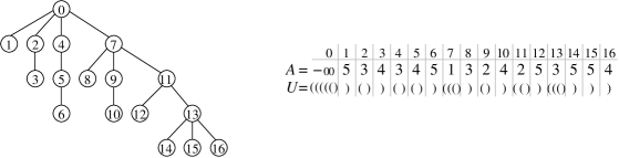
Figure 1: The LRM-Tree $\mathcal{T}_{A}$ of the input array $A$, and its DFUDS $U$.

The following lemma shows a simple way to construct the LRM-Tree in linear time (Fischer [8] gave a more complicated linear-time algorithm with advantages that are irrelevant for this paper.)

Lemma 3.

There is an algorithm computing the LRM-Tree of an array of $n$ integers in at most $2n$ data comparisons.

Proof.

The computation of the LRM-Tree corresponds to a simple scan over the input array, starting at $A[0]=-\infty$, building down iteratively the current rightmost branch of the tree with increasing elements of the sequence till an element $x$ smaller than its predecessor is encountered, at which point one climbs the right-most branch up to the first node $v$ holding a value smaller than $x$, and starts a new branch with a right-most child of $v$ of value $x$. As the root of the tree has value $A[0]=-\infty$ smaller than all elements, the algorithm always terminates.

The construction algorithm performs at most $2n$ comparisons. Charging the last comparison performed during the insertion of an element $x$ to $x$ itself, and all previous comparisons to the elements already in the LRM-Tree, each element is charged at most twice: once when it is inserted into the tree, and once when scanning it while searching for a smaller value on the rightmost branch. As in the latter case all scanned elements are removed from the rightmost path, this second charging occurs at most once for each element. ∎

2.4 Range Minimum Queries

We consider the following queries on a static array $A[1,n]$ (parameters $i$ and $j$ with $1\leq i\leq j\leq n$):

Definition 4 (Range Minimum Queries).

$\text{\sc rmq}_{A}(i,j)=$ position of the minimum in $A[i,j]$.

RMQs have a wide range of applications for various data structures and algorithms, including text indexing [10], pattern matching [6], and more elaborate kinds of range queries [5].

The connection between LRM-Trees and RMQs is given as follows. For two given nodes $i$ and $j$ in a tree $T$, let $\text{\sc lca}_{T}(i,j)$ denote their Lowest Common Ancestor (LCA), which is the deepest node that is an ancestor of both $i$ and $j$. Now let $\mathcal{T}_{A}$ be the LRM-Tree of $A$. For arbitrary nodes $i$ and $j$ in $\mathcal{T}_{A}$, $1\leq i<j\leq n$, let $\ell=\text{\sc lca}_{\mathcal{T}_{A}}(i,j)$. Then if $\ell=i$, $\text{\sc rmq}_{A}(i,j)$ is given by $i$, and otherwise, $\text{\sc rmq}_{A}(i,j)$ is given by the child of $\ell$ that is on the path from $\ell$ to $j$ [8].

Since there are succinct data structures supporting the LCA operator in succinctly encoded trees in constant time, this yields a succinct index:

Lemma 5 (Fischer[8]).

For an array $A[1,n]$ of totally ordered objects, there is a non-systematic succinct index using $2n+o(n)$ bits and supporting RMQs in zero data queries and ${\cal O}(1)$ index queries. This index can be built using at most ${\cal O}(n)$ data comparisons.

Two problems with this proof (hence I removed it): 1) if it was already given in your paper, we should not give it again, and if it is different we should explain why (and maybe not cite your paper in its title). 2) More importantly, it does not prove the linear time construction of the RMQ index. Does your paper prove it? ad 2: YES OF COURSE I prove it!

Proof.

We encode the LRM-Tree $\mathcal{T}_{A}$ by its Depth-First Unary Degree Sequence (DFUDS) $U$ using $2n$ bits [benoit05representing]. In $U$, nodes are listed in preorder, where node $i$ with $k$ children is encoded as $k$ opening parentheses and one closing parenthesis (a single opening parenthesis is prepended to $U$ to make it balanced). As the nodes in $\mathcal{T}_{A}$ appear in preorder, we can jump to the description of node $i$ (corresponding to index $i$ in $A$) by a single select-statement in $U$. Further, there are $o(n)$-bit indices for DFUDS for computing LCAs in ${\cal O}(1)$ time [8]. By the discussion above, from the LCA we can compute the range minimum. ∎

2.5 Adaptive Sorting, and Compression of Permutations

Sorting a permutation of $n$ elements in the comparison model typically requires $\Omega(n\lg n)$ comparisons in the worst case. Yet, better results can be achieved for some parameterized classes of permutations. Among others, Knuth [17] considered Runs (ascending subsequences), counted by $\mathsf{nRuns}(\pi)=1+|\{i~{}:\ 1<i\leq n,\pi_{i+1}<\pi_{i}\}|;$ Levcopoulos and Petersson [18] introduced Shuffled Up Sequences, counted by $\mathsf{nSUS}(\pi)=\min\{k:\pi\textrm{ is covered by }k\textrm{ increasing subsequences}\},$ and Shuffled Monotone Sequences, counted by $\mathsf{nSMS}(\pi)=\min\{k:\pi\textrm{ is covered by }k\textrm{ monotone subsequences}\};$ and Barbay and Navarro [2] introduced strict variants of those concepts, namely Strict Runs and Strict Shuffled Up Sequences, where sorted subsequence are composed of consecutive integers (e.g. $(\mathbf{2,3,4},1,\mathit{5,6,7,8})$ has two runs but three strict runs), counted by $\mathsf{nSRuns}$ and $\mathsf{nSSUS}$, respectively. For any “measure of disorder” $\mathsf{X}$ among those five, there is a variant of the merge-sort algorithm which sorts a permutation $\pi$ of size $n$ and measure $\mathsf{X}$ in time ${\cal O}((n+1)\lg\mathsf{X})$, which is optimal in the worst case among instances of fixed size $n$ and fixed values of $\mathsf{X}$ (this is not necessarily true for other measures of disorder).

As the merging cost induced by a subsequence is increasing with its length, the sorting time of a permutation can be improved by rebalancing the merging tree [2]. This merging cost is actually equivalent to the cost of encoding, for each element of the sorted permutation, the subsequence of origin of this element. Hence rebalancing the merging tree is equivalent to optimize a code for those addresses, and can be done via a Huffman tree [14]. The complexity can then be expressed more precisely in function of the entropy of the relative sizes of the sorted subsequences identified, where the entropy ${\cal H}(\mathsf{Seq})$ of a sequence $\mathsf{Seq}=\langle n_{1},n_{2},\dots,n_{r}\rangle$ of $r$ positive integers adding up to $n$ is ${\cal H}(\mathsf{Seq})=\sum_{i=1}^{r}\frac{n_{i}}{n}\lg\frac{n}{n_{i}}$, which satisfies $(r-1)\lg n\leq n{\cal H}(\mathsf{Seq})\leq n\lg r$ (by concavity of the logarithm).

Simplified the inequality (by multiplying each term by n), and realized it was different from the one Gonzalo used for STACS 2010: yours was saying $\frac{r\lg n}{n}\leq{\cal H}(\mathsf{Seq})\leq\lg r$ (by convexity of the logarithm)., which is equivalent to $r\lg n\leq n{\cal H}(\mathsf{Seq})\leq n\lg r$. I did not have the time to check it and put the one from Gonzalo?

Also, I corrected “(by convexity of the logarithm)”: the logarithm is concave and not convex (check http://en.wikipedia.org/wiki/Concave_function if in doubt).

Barbay and Navarro [2] observed that each such algorithm from the comparison model also describes an encoding of the permutation $\pi$ that it sorts, so that it can be used to compress permutations from specific classes to less than the information-theoretic lower bound of $n\lg n$ bits. Furthermore they used the similarity of the execution of the merge-sort algorithm with a Wavelet Tree [13], to support the application of $\pi()$ and its inverse $\pi^{-1}()$ in time logarithmic in the disorder of the permutation $\pi$ as measured by $\mathsf{nRuns}$, $\mathsf{nSRuns}$, $\mathsf{nSUS}$, $\mathsf{nSSUS}$ and $\mathsf{nSMS}$, respectively) in the worst case. We summarize their technique in Lemma 6 below, in a way independent of the partition chosen for the permutation.

Lemma 6 (Barbay et al. [2]).

Given a partition $\mathsf{Seq}$ of a permutation $\pi$ of $n$ elements into $\mathsf{nSeq}$ sorted subsequences of respective lengths $\mathsf{Seq}$, these subsequences can be merged with $n(1+{\cal H}(\mathsf{Seq}))$ comparisons on $\pi$ and ${\cal O}(\mathsf{nSeq}\lg\mathsf{nSeq})$ internal operations, and this merging can be encoded using at most $(1+{\cal H}(\mathsf{Seq}))(n+o(n))+{\cal O}(\mathsf{nSeq}\lg n)$ bits so that it supports the computation of $\pi(i)$ and $\pi^{-1}(i)$ in time ${\cal O}(1+\lg\mathsf{nSeq})$ in the worst case and in time ${\cal O}(1+{\cal H}(\mathsf{Seq}))$ on average when $i$ is chosen uniformly at random in $[1..n]$.

3 Compressed Succinct Indexes for Range Minima

We now explain how to improve on the result from Lemma 5 for permutations that are partially ordered. Without loss of generality, we consider only the case where the input is a permutation of $[1..n]$: if this is not the case, we can sort the elements in $A$ by rank, considering earlier occurrences of equal elements as smaller.

3.1 Strict Runs

The simplest compressed data structure for RMQs uses an amount of space which is a function of $\mathsf{nSRuns}$, the number of strict runs in $\pi$. It uses $2\mathsf{nSRuns}+o(n)$ bits on permutations where $\mathsf{nSRuns}\in o(n)$:

Theorem 1.

There is a non-systematic compressed succinct index using $2\mathsf{nSRuns}+\lceil\lg{n\choose\mathsf{nSRuns}}\rceil+o(n)$ bits and supporting RMQs in zero data queries and ${\cal O}(1)$ index queries. Add Construction time, in the text and in the proof.

Proof.

We mark the beginnings of each runs in $A$ with a 1 in a bit-vector $B[1,n]$, and represent $B$ with the compressed succinct data structure from Raman et al. [23], using $\lceil\lg{n\choose\mathsf{nSRuns}}\rceil+o(n)$ bits. Further, we define $A^{\prime}$ as the (conceptual) array consisting of the heads of $A$’s runs ($A^{\prime}[i]=A[\textit{select}_{1}(B,i)]$). We build the LRM-Tree from Lemma 5 on $A^{\prime}$; using $2\mathsf{nSRuns}(1+o(1))$ bits. To answer a query $\text{\sc rmq}_{A}(i,j)$, compute $x=\textit{rank}_{1}(B,i)$ and $y=\textit{rank}_{1}(B,j)$, and compute $m^{\prime}=\text{\sc rmq}_{A^{\prime}}(x,y)$ as a range minimum in $A^{\prime}$, and map it back to its position in $A$ by $m=\textit{select}_{1}(B,m^{\prime})$. Then if $m<i$, return $i$ as the final answer to $\text{\sc rmq}_{A}(i,j)$, otherwise return $m$. The correctness from this algorithm follows from the fact that only $i$ and the heads of strict runs that are entirely contained in the query interval can be the range minimum; the former occurs if and only if the head of the run containing $i$ is smaller than all other heads in the query range. ∎

Obviously, this compressed data-structure is interesting only if $\mathsf{nSRuns}\in o(n)$. We explore in the following section a more general measure of partial order, $\mathsf{nRuns}$.

3.2 General Runs

The same idea as in Theorem 1 applied to more general runs yields another compressed succinct index for RMQs, potentially smaller but this time requiring to access the input to answer RMQs.

Theorem 2.

There is a systematic compressed succinct index using $2\mathsf{nRuns}+\lceil\lg{n\choose\mathsf{nRuns}}\rceil+o(n)$ bits and supporting RMQs in $1$ data comparison and ${\cal O}(1)$ index operations. Add Construction time, in the text and in the proof.

Proof.

We build the same data structures as in Theorem 1, now using $2\mathsf{nRuns}+\lceil\lg{n\choose\mathsf{nRuns}}\rceil+o(n)$ bits. To answer a query $\text{\sc rmq}_{A}(i,j)$, compute $x=\textit{rank}_{1}(B,i)$ and $y=\textit{rank}_{1}(B,j)$. If $x=y$, return $i$. Otherwise, compute $m^{\prime}=\text{\sc rmq}_{A^{\prime}}(x+1,y)$, and map it back to its position in $A$ by $m=\textit{select}_{1}(B,m^{\prime})$. The final answer is $k$ if $A[k]<A[m]$, and $m$ otherwise. ∎

To achieve a non-systematic compressed succinct index whose space usage is a function of $\mathsf{nRuns}$, we need more space and a more heavy machinery, as shown next. The main idea is that a permutation with few runs results in a compressible LRM-Tree, where many nodes have out-degree 1.

Theorem 3.

There is a non-systematic compressed succinct index using $2\mathsf{nRuns}\lg n+o(n)$ bits, and supporting RMQs in zero data comparisons and ${\cal O}(1)$ index operations. Add Construction time, in the text and in the proof.

Proof.

We build the LRM-Tree $\mathcal{T}_{A}$ from Sect. 2.3 directly on $A$, and then compress it with the tree-compressor due to Jansson et al. [16].

To see that this results in the claimed space, let $n_{k}$ denote the number of nodes in $\mathcal{T}_{A}$ with out-degree $k\geq 0$. Let $(i_{1},j_{1}),\dots,(i_{\mathsf{nRuns}},j_{\mathsf{nRuns}}])$ be an encoding of the runs in $A$ as (start, end), and look at a pair $(i_{x},j_{x})$. We have $\text{\sc psv}_{A}(k)=k-1$ for all $k\in[i_{x}+1..j_{x}]$, and so the nodes in $[i_{x}..j_{x}]$ form a path in $\mathcal{T}_{A}$, possibly interrupted by branches stemming from heads $i_{y}$ of other runs $y>x$ with $\text{\sc psv}_{A}(i_{y})\in[i_{x}..j_{x}-1]$. Hence $n_{0}=\mathsf{nRuns}$, and $n_{1}\geq n-\mathsf{nRuns}-(\mathsf{nRuns}-1)\geq n-2\mathsf{nRuns}$, as in the worst case the values $\text{\sc psv}_{A}(i_{y})$ for $i_{y}\in\{i_{2},i_{3},\dots,i_{\mathsf{nRuns}}\}$ are all different.

Now $\mathcal{T}_{A}$, with degree-distribution $n_{0},\dots,n_{n-1}$, is compressed into $nH^{*}(\mathcal{T}_{A})+O\left(\frac{n\lg^{2}n}{\lg n}\right)$ bits, where

$$nH^{*}(\mathcal{T}_{A})=\lg\left(\frac{1}{n}\binom{n}{n_{0}n_{1}\dots n_{n-1}}\right)$$

is the so-called tree entropy [16] of $\mathcal{T}_{A}$. This representation supports all navigational operations in $\mathcal{T}_{A}$ in constant time, and in particular those required for Lemma 5. A rough inequality yields a bound on the number of possible LRM-Trees:

$$\binom{n}{n_{0}n_{1}\dots n_{n-1}}=\frac{n!}{n_{0}!n_{1}!\dots n_{n-1}!}\leq\frac{n!}{n_{1}!}\leq\frac{n!}{(n-2\mathsf{nRuns})!}\leq n^{2\mathsf{nRuns}}\ ,$$

$$\binom{n}{n_{0}n_{1}\dots n_{n-1}} = \frac{n!}{n_{0}!n_{1}!\dots n_{n-1}!}$$

$$\leq \frac{n!}{n_{1}!}$$

$$\leq \frac{n!}{(n-2\mathsf{nRuns})!}$$

$$\leq n^{2\mathsf{nRuns}}\ ,$$

from which one easily bounds the space usage of the compressed succinct index:

$$nH^{*}(T)\leq\lg\left(\frac{1}{n}n^{2\mathsf{nRuns}}\right)=\lg\left(n^{2\mathsf{nRuns}-1}\right)=(2\mathsf{nRuns}-1)\lg n\leq 2\mathsf{nRuns}\lg n\ .$$

$$nH^{*}(T) \leq \lg\left(\frac{1}{n}n^{2\mathsf{nRuns}}\right)$$

$$= \lg\left(n^{2\mathsf{nRuns}-1}\right)$$

$$= (2\mathsf{nRuns}-1)\lg n$$

$$\leq 2\mathsf{nRuns}\lg n\ .$$

Adding the space required to index the structure of Jansson et al. [16] yields the desired space. ∎

3.3 Range Quantile Queries

We now turn our attention to range quantile queries.

Theorem 4.

There is a non-systematic preprocessing scheme for ${\cal O}(\lg\mathsf{nSSUS})$-RQQs that needs $n(2+H(\mathsf{SSUS}))(1+o(1))$ bits. If $p$ is chosen uniformly at random in $[1..n]$ then the average time to answer $\text{\sc rqq}_{A}(\cdot,\cdot,p)$ is ${\cal O}(1+H(\mathsf{SSUS}))$.

Proof.

Our basis is the approach of Gfeller and Sanders [gfeller09towards], also described by Gagie et al. [gagie09range], that represents $A$ by a binary wavelet tree [13]. The difference is that the shape of the wavelet tree is not perfectly balanced, but determined by the tree resulting from running the Hu-Tucker algorithm [hu71optimum] on $\mathsf{SSUS}$. In particular, let $[i_{1}..j_{1}],\dots,[i_{\mathsf{nSSUS}}..j_{\mathsf{nSSUS}}]$ be the shuffled up-sequences with $i_{0}=1,i_{x}=j_{x-1}+1$ for $2\leq x\leq\mathsf{nSSUS}$, and $j_{\mathsf{nSSUS}}=n$. Then $\mathsf{SSUS}=\langle y_{1},\dots,y_{\mathsf{nSSUS}}\rangle$ with $y_{x}=j_{x}-i_{x}+1$, and the Hu-Tucker algorithm produces a binary tree $T$ where the $k$’th leftmost leaf $\ell_{k}$ represents the interval $[i_{k}..j_{k}]$, and $L=\sum y_{k}\textit{depth}(\ell_{k})$ is minimal. Moreover, $L<n(2+H(\mathsf{SSUS}))$.

We enhance $T$ with the usual structures of a wavelet tree: every node $v$ (implicitly) stores an subsequence $A_{v}[1,n_{v}]$ of the original array $A$ (the root stores the complete array $A[1,n]$). An associated bit-vector $B_{v}[1,n_{v}]$ indicates which characters from $A_{v}$ can be found in the left or right child of $v$: $B_{v}[i]=0$ iff $A_{v}[i]\in[i_{k}..j_{k}]$, and the $k$’th leftmost leaf is in the subtree rooted at $v$’s left child. Bet-vectors $B_{v}$ also define the sequences of their respective children in a natural way. This process continues recursively until we have reached a leaf of $T$, where no information is stored.

Now a query $\text{\sc rqq}_{A}(i,j,p)$ proceeds as in the original algorithm [gfeller09towards], working its way down the tree while adapting $i$, $j$, and $k$ accordingly. Now suppose we have reached a leaf $\ell$ with values $i^{\prime}$, $j^{\prime}$, and $p^{\prime}$. There, we search for the position of the $p^{\prime}$’th smallest element in $A_{\ell}$. But $A_{\ell}=[i_{k}..j_{k}]$ for some $k$, so the answer is simply $i^{\prime}+p^{\prime}-1$.

Because the depth of $T$ is at most $\mathsf{nSSUS}$, the claim on worst-case time follows. The claim on average time follows from the fact that the average depth of $T$ is given by $H(\mathsf{SSUS})$. ∎

4 Sorting Permutations

Barbay and Navarro [2] showed how to use the decomposition of a permutation $\pi$ in $\mathsf{nRuns}$ ascending consecutive runs of respective lengths $\mathsf{Runs}$ to sort adaptively to their entropy ${\cal H}(\mathsf{Runs})$. Those runs entirely partition the LRM-Tree of $\pi$ into $\mathsf{nRuns}$ paths, each starting at some branching node of the tree, and ending at a leaf: one can easily draw this partition by iteratively tagging the leftmost maximal untagged up-from-leaf path of the LRM-Tree.

Yet, any partition of the LRM-Tree into down paths (so that the values traversed by the path are increasing) can be used to sort $\pi$. Since there are exactly $\mathsf{nRuns}$ leaves in the LRM-Tree, no such partition can be smaller than the partition of $\pi$ into ascending consecutive runs. But in the case where some of those partitions are more imbalanced than the original one, this yields a partition of smaller entropy, and hence a faster sorting algorithm. We define a family of such partitions:

Definition 7 (LRM-Partition).

A LRM-Partition of a permutation $\pi$ with LRM-Tree $\mathcal{T}_{\pi}$ is defined recursively as follows. One subsequence is the “spinal chord” of $\mathcal{T}_{\pi}$, one of the longest root-to-leaf paths in $\mathcal{T}_{\pi}$. Removing this spinal chord of $\mathcal{T}_{\pi}$ leaves a forest of more shallow trees. The rest of the partition is obtained by computing and concatenating some LRM-partitions of those trees.

This definition does not define a unique partition, but a family of partitions: there might be several ways to choose the “spinal chord” of each subtree when several nodes have the same depth, and of course the order of the subsequences in the partition does not matter either. Yet, there will always be $\mathsf{nRuns}$ many subsequences in the partition, and any LRM-Partition is never worse and often better (in terms of sorting and compressing) than the the original Run-Partition. The situation is similar to the one of ${\cal H}(\mathsf{SUS})$ versus $\mathsf{nSUS}$: it is easier to minimize $\mathsf{nSUS}$ (resp. $\mathsf{nRuns}$) than ${\cal H}(\mathsf{SUS})$ (resp. ${\cal H}(\mathsf{LRM})$), yet one can take advantage of the entropy of a partition minimizing $\mathsf{nSUS}$ (resp. of a LRM-Partition).

Note that each down-path of the LRM-Tree corresponds to an ascending subsequence of $\pi$, but not all ascending subsequences correspond to down-paths of the LRM-Tree, hence partitioning optimally $\pi$ into $\mathsf{nSUS}$ ascending subsequences potentially yields smaller partitions, or ones of smaller entropy: the LRM-partitions seem inferior to SUS-partitions. Yet, the fact which make LRM-Partitions particularly interesting is that it can be computed in linear time (which is not true for SUS-Partitions):

Lemma 8.

There is an algorithm finding one of the LRM-Partitions of a permutation $\pi$ of size $n$ in ${\cal O}(n)$ data comparisons.

Proof.

Definition 7 is constructive: we are only left to show that this algorithm can be executed in linear time. Having built $\mathcal{T}_{A}$ using Lemma 3 in $2n$ comparisons, we first set up an array $D$ containing the depths of the nodes in $\mathcal{T}_{A}$, listed in preorder. We then index $D$ for range maximum queries in linear time using Lemma 5.

Now the deepest node in $\mathcal{T}_{A}$ can be found by a range maximum query over the whole array, supported in constant time. From this node, we follow the path to the root, and save the corresponding nodes as the first subsequence. This divides $A$ into disconnected subsequences, which can be processed recursively using the same algorithm, as the nodes in any sub-tree of $\mathcal{T}_{A}$ form an interval in $D$. We do so until all elements in $A$ have been assigned to a subsequence.

Note that in the recursive steps, the numbers in $D$ are not anymore the depths of the corresponding nodes in the remaining sub-trees. But as all depths listed in $D$ differ by the same offset from their depths in any connected subtree, this does not affect the result of the range maximum query. ∎

Given a LRM-Partition of the permutation $\pi$, sorting $\pi$ is just a matter of applying Lemma 6:

Theorem 5.

Let $\pi$ be a permutation of size $n$. Identifying its $\mathsf{nRuns}$ runs by building the LRM-Tree through Lemma 3, obtaining a LRM-Partition of subsequences of respective lengths $\mathsf{LRM}$ through Lemma 8, and merging the subsequences of this partition through Lemma 6, results in an algorithm sorting $\pi$ in a total of $n(3+{\cal H}(\mathsf{LRM}))$ data comparisons and ${\cal O}(n+\mathsf{nRuns}\lg\mathsf{nRuns})$ internal operations, accounting for a total time of ${\cal O}(n(1+{\cal H}(\mathsf{LRM})))$.

Proof.

Lemma 3 builds the LRM-Tree in $2n$ data comparisons, Lemma 8 extract from it a LRM-Partition in ${\cal O}(n)$ internal operations, and Lemma 6 merges the subsequences of the LRM-Partition in $n(1+{\cal H}(\mathsf{LRM}))$ data comparisons and ${\cal O}(\mathsf{nRuns}\lg\mathsf{nRuns})$ internal operations. The sum of those complexities yields $n(3+{\cal H}(\mathsf{LRM}))$ data comparisons and ${\cal O}(n+\mathsf{nRuns}\lg\mathsf{nRuns})$ internal operations.

Since $\mathsf{nRuns}\lg\mathsf{nRuns}<n{\cal H}(\mathsf{LRM})+\lg\mathsf{nRuns}$ by concavity of the logarithm, the total time complexity is in ${\cal O}(n(1+{\cal H}(\mathsf{LRM})))$. ∎

Since by construction ${\cal H}(\mathsf{LRM})\leq{\cal H}(\mathsf{Runs})$, this result naturally improves on the adaptive merge sort algorithm for runs [2]. However, ${\cal H}(\mathsf{SUS})$ can be arbitrarily smaller than ${\cal H}(\mathsf{LRM})$: this means that, in the worst case over instances of fixed $n$ and ${\cal H}(\mathsf{SUS})$, SUS sorting has a strictly better asymptotical complexity than LRM sorting; while, in the worst case over instances of fixed $n$ and ${\cal H}(\mathsf{LRM})$, SUS sorting has the same asymptotical complexity than LRM sorting. “instances of fixed $n$ and ${\cal H}(\mathsf{LRM})$” is not well defined, since ${\cal H}(\mathsf{LRM})$ is not uniquely defined…

Yet, on instances where ${\cal H}(\mathsf{LRM})<2{\cal H}(\mathsf{SSUS})-1$, LRM-Sorting actually performs less data comparisons (and potentially more index operations) than SUS-Sorting. Barbay et al.’s improvement [2] of SUS-Sorting performs $2n(1+{\cal H}(\mathsf{SUS})$ data comparisons, decomposed into $n(1+{\cal H}(\mathsf{SUS}))$ data comparisons to compute a partition $\pi$ into $\mathsf{nSUS}$ sub-sequences which is minimal in size, if not necessarily in entropy; and $n(1+{\cal H}(\mathsf{SUS}))$ data comparisons (and ${\cal O}(n+\mathsf{nSUS}\lg\mathsf{nSUS})$ internal operations) to merge the subsequences into a single ordered one. On the other hand, the combination of Lemma 3 with Lemma 8 yields a LRM-Partition in $2n$ data comparisons and ${\cal O}(n)$ index operations; which is then merged in $n(1+{\cal H}(\mathsf{LRM}))$ data comparisons (and ${\cal O}(n+\mathsf{nRuns}\lg\mathsf{nRuns})$ internal operations) to merge the subsequences into a single ordered one. Comparing the $2n(1+{\cal H}(\mathsf{SUS})$ data comparisons of SUS-Sorting with the $n(3+{\cal H}(\mathsf{LRM}))$ data comparisons of LRM-Sorting shows that on instance where ${\cal H}(\mathsf{LRM})<2{\cal H}(\mathsf{SUS})-1$, LRM-Sorting performs less data comparisons (only potentially twice less, given that ${\cal H}(\mathsf{SUS})\leq{\cal H}(\mathsf{LRM})$. This comes to the price of potentially more internal operations: SUS-Sorting performs ${\cal O}(n+\mathsf{nSUS}\lg\mathsf{nSUS})$ such ones while LRM-Sorting performs ${\cal O}(n+\mathsf{nRuns}\lg\mathsf{nRuns})$ such ones, and $\mathsf{nSUS}\leq\mathsf{nRuns}$ by definition.

When considering external memory, this is important in the case where the data does not fit in main memory while the internal data-structures (using much less space than the data itself) of the algorithms do: then data comparisons are much more costly than internal operations. Furthermore, we show in the next section that this difference of performance implies an even more meaningful difference in the size of the permutation encodings corresponding to the sorting algorithms.

5 Compressing Permutations

As shown by Barbay and Navarro [2], sorting opportunistically in the comparison model yields a compression scheme for permutations, and sometimes a compressed succinct data structure supporting the direct and inverse operators in reasonable time. We show that this time again the sorting algorithm of Theorem 5 corresponds to a compressed succinct data structure for permutations which supports the direct and reverse operators in good time, while often using less space than previous solutions. The essential component of our solution is a data structure encoding the LRM-Partition. In order to apply Lemma 6, our data structure must support two operators in good time:

• the first operator, $\textit{map}(i)$, consists of indicating, for each position $i\in[1..n]$ in the input permutation $\pi$, the corresponding subsequence $s$ of the LRM-Partition, and the relative position $p$ of $i$ in this subsequence;

• the second operator, $\textit{unmap}(s,p)$ is just the reverse of the previous one: given a subsequence $s\in[1..\mathsf{nRuns}]$ of the LRM-Partition of $\pi$ and a position $p\in[1..n_{s}]$ in it, the operator must indicate the corresponding position $i$ in $\pi$.

We obviously cannot afford to rewrite the numbers of $\pi$ in the order described by the partition, which would use $n\lg n$ bits. A naive solution would be to encode this partition as a string $S$ over alphabet $[1..\mathsf{nRuns}]$, using a succinct data structure supporting the access, rank and select operators on it. This solution is not suitable as it would require at the very least $n{\cal H}(\mathsf{Runs})$ bits only to encode the LRM-Partition, making this encoding worse than the $\mathsf{nRuns}$ compressed succinct data structure [2]. We describe a more complex data structure which uses linear space, and supports the desired operators in constant time.

Lemma 9.

Let $P$ be a LRM-Partition consisting of $\mathsf{nRuns}$ subsequences of respective lengths $\mathsf{LRM}$, summing to $n$. There is a succinct data structure using $2(n+\mathsf{nRuns})+o(n)$ bits and supporting the operators map and unmap on $P$ in constant time.

Proof.

The main idea of the data structure is that the subsequences of a LRM-Partition for a permutation $\pi$ are not as general as, say, the subsequences of the partition into $\mathsf{nSUS}$ up-sequences. For each pair of subsequences $(u,v)$, either the positions of $u$ and $v$ belongs to distinct intervals of $\pi$, or the values corresponding to $u$ (resp. $v$) all fall between two values from $v$ (resp. $u$).

As such, the subsequences of the LRM-Partition can be organized into a forest of ordinal trees, where the internal nodes of the trees correspond to the $\mathsf{nRuns}$ subsequences of the LRM-Partition, organized so that $u$ is parent of $v$ if the positions of $v$ are contained between two positions of $u$, and where the leaves of the trees correspond to the $n$ positions in $\pi$, children of the internal node $u$ corresponding to the subsequence they belong to. For instance, the permutation $\pi=(4,5,9,6,8,1,3,7,2)$ has a unique LRM-Partition $\{(4,5,6,8),(9),(1,3,7),(2)\}$, whose encoding can be visualized by the expression $(45(9)68)(137)(2)$ and encoded by the balanced parenthesis expression $(()()(())()())(()()())(())$ (note that this is a forest, not a tree, hence the excess of ’(’s versus ’)’s is going to zero several times inside the expression).

Given a position $i\in[1..n]$ in $\pi$, the corresponding subsequence $s$ of the LRM-Partition is simply obtained by finding the parent of the $i$-th leaf, and returning its preorder rank among internal nodes. The relative position $p$ of $i$ in this subsequence is given by the number of its left siblings which are leaves. Given a subsequence $s\in[1..\mathsf{nRuns}]$ of the LRM-Partition of $\pi$ and a position $p\in[1..n_{s}]$ in it, the corresponding position $i$ in $\pi$ is computed by finding the $s$-th internal node in preorder, selecting its $p$-th child which is a leaf, and computing the preorder rank of this node among all the leaves of the tree.

We represent such a forest using a Balanced Parentheses Sequence using $2(n+\mathsf{nRuns})+o(n)$ bits and enhance it with a $o(n)$-bit succinct index [24] supporting in constant time the operators rank and select on leaves (i.e., on the pattern ’()’), and rank and select on internal nodes (i.e., on the pattern ’((’). With these operators we can simulate all operations described in the previous paragraph. ∎

Given the data structure for LRM-Partitions from Lemma 9, applying the merging data structure from Lemma 6 immediately yields a compressed succinct data structure for permutations. Note that this encoding is not a succinct index, so that it would not make any sense to measure its space complexity in term of data and index complexity.

Theorem 6.

Let $\pi$ be a permutation of size $n$ and $P$ a LRM-Partition for $\pi$ consisting of $\mathsf{nRuns}$ subsequences of respective lengths $\mathsf{LRM}$. There is a compressed succinct data structure using $(1+{\cal H}(\mathsf{LRM}))(n+o(n))+{\cal O}(\mathsf{nRuns}\lg n)$ bits, supporting the computation of $\pi(i)$ and $\pi^{-1}(i)$ in time ${\cal O}(1+\lg\mathsf{nRuns})$ in the worst case, and in time ${\cal O}(1+{\cal H}(\mathsf{LRM}))$ on average when $i$ is chosen uniformly at random in $[1..n]$, and which can be computed in the times indicated in Theorem 5, summing to ${\cal O}(n(1+{\cal H}(\mathsf{LRM})))$.

Proof.

Lemma 9 yields a data structure for a LRM-Partition of $\pi$ using $2(n+\mathsf{nRuns})+o(n)$ bits, and supports the map and unmap operators in constant time. The merging data structure from Lemma 6 requires $(1+{\cal H}(\mathsf{LRM}))(n+o(n))+{\cal O}(\mathsf{nRuns}\lg n)$ bits, and supports the operators $\pi()$ and $\pi^{-1}()$ in the time described, through the additional calls to map and unmap. Summing both spaces yields the desired final space. ∎

Jeremy, pls carefully check the above. I did, I think. One confusion I have: Computing the Hufman takes only $\mathsf{nSeq}\lg\mathsf{nSeq}$ comparisons, but encoding the lengths of the runs requires something like $\mathsf{nSeq}\lg n$ bits. This is smaller than $n$ bits anyway so we could hide it away.

6 Conclusion and Future Work

One additional result not described here is how to take advantage of strict runs, in addition of taking advantage of general runs, for LRM sorting and encoding of permutation. Another related result is a variant of LRM-Trees, Roller Coaster Trees (RC-Trees), which take advantage of permutations formed by the combinations of ascending and descending runs. This approach is trivial when considering subsequences of consecutive positions, gets slightly technical when considering the insertion of descending runs, and requires new techniques to adapt the compressed succinct data structure to this new setting. Since the optimal partitioning into up and down sequences when considering general subsequences requires exponential time, RC-Sorting seems a much desirable improvement on merging ascending and descending runs, as well as a more practical alternative to SMS-Sorting, in the same way as LRM-Tree improved on Runs-Sorting while staying more practical than SUS-Sorting. Another result to come is the generalization of our results to the indexing, sorting and compression of general sequences (i.e., also to integer functions), But we do support RMQs for general sequences, don’t we? (It’s what we claim, and we discussed it a while ago.) taking advantage of the redundancy in a general sequence to sort faster and encode in even less space, in function of both the entropy of the frequencies of the symbols and the entropy of the lengths of the subsequences of the LRM-Partition. Finally, studying the integration of those compressed data structures into compressed text indexes like suffix arrays [21] is likely to yield interesting results, too.

Appendix A Proof of Lemma 6

References

- [1] J. Barbay, M. He, J. I. Munro, and S. S. Rao. Succinct indexes for strings, binary relations, and multi-labeled trees. In Proc. SODA, pages 680–689. ACM/SIAM, 2007.
- [2] J. Barbay and G. Navarro. Compressed representations of permutations, and applications. In Proc. STACS, pages 111–122. IBFI Schloss Dagstuhl, 2009.
- [3] M. A. Bender, M. Farach-Colton, G. Pemmasani, S. Skiena, and P. Sumazin. Lowest common ancestors in trees and directed acyclic graphs. J. Algorithms, 57(2):75–94, 2005.
- [4] G. S. Brodal, P. Davoodi, and S. S. Rao. On space efficient two dimensional range minimum data structures. In Proc. ESA (Part II), volume 6347 of LNCS, pages 171–182. Springer, 2010.
- [5] K.-Y. Chen and K.-M. Chao. On the range maximum-sum segment query problem. In Proc. ISAAC, volume 3341 of LNCS, pages 294–305. Springer, 2004.
- [6] M. Crochemore, C. S. Iliopoulos, M. Kubica, M. S. Rahman, and T. Walen. Improved algorithms for the range next value problem and applications. In Proc. STACS, pages 205–216. IBFI Schloss Dagstuhl, 2008.
- [7] C. Daskalakis, R. M. Karp, E. Mossel, S. Riesenfeld, and E. Verbin. Sorting and selection in posets. In Proc. SODA, pages 392–401. ACM/SIAM, 2009.
- [8] J. Fischer. Optimal succinctness for range minimum queries. In Proc. LATIN, volume 6034 of LNCS, pages 158–169. Springer, 2010.
- [9] J. Fischer, V. Heun, and H. M. Stühler. Practical entropy bounded schemes for -range minimum queries. In Proc. DCC, pages 272–281. IEEE Press, 2008.
- [10] J. Fischer, V. Mäkinen, and G. Navarro. Faster entropy-bounded compressed suffix trees. Theor. Comput. Sci., 410(51):5354–5364, 2009.
- [11] A. Gál and P. B. Miltersen. The cell probe complexity of succinct data structures. Theor. Comput. Sci., 379(3):405–417, 2007.
- [12] A. Golynski. Optimal lower bounds for rank and select indexes. Theor. Comput. Sci., 387(3):348–359, 2007.
- [13] R. Grossi, A. Gupta, and J. S. Vitter. High-order entropy-compressed text indexes. In Proc. SODA bla, pages 841–850. ACM/SIAM, 2003.
- [14] D. Huffman. A method for the construction of minimum-redundancy codes. In Proceedings of the I.R.E., volume 40, pages 1090–1101, 1952.
- [15] G. Jacobson. Space-efficient static trees and graphs. In Proc. FOCS, pages 549–554. IEEE Computer Society, 1989.
- [16] J. Jansson, K. Sadakane, and W.-K. Sung. Ultra-succinct representation of ordered trees. In Proc. SODA, pages 575–584. ACM/SIAM, 2007.
- [17] D. E. Knuth. Art of Computer Programming, Volume 3: Sorting and Searching (2nd Edition). Addison-Wesley Professional, April 1998.
- [18] C. Levcopoulos and O. Petersson. Sorting shuffled monotone sequences. Inf. Comput., 112(1):37–50, 1994.
- [19] V. Mäkinen and G. Navarro. Implicit compression boosting with applications to self-indexing. In Proc. SPIRE, LNCS 4726, pages 214–226. Springer, 2007.
- [20] J. I. Munro, R. Raman, V. Raman, and S. S. Rao. Succinct representations of permutations. In Proc. ICALP, volume 2719 of LNCS, pages 345–356. Springer, 2003.
- [21] G. Navarro and V. Mäkinen. Compressed full-text indexes. ACM Computing Surveys, 39(1):Article No. 2, 2007.
- [22] M. Pǎtraşcu. Succincter. In Proc. FOCS, pages 305–313. IEEE Computer Society, 2008.
- [23] R. Raman, V. Raman, and S. S. Rao. Succinct indexable dictionaries with applications to encoding -ary trees and multisets. ACM Transactions on Algorithms, 3(4):Article No. 43, 2007.
- [24] K. Sadakane. Compressed suffix trees with full functionality. Theory of Computing Systems, 41(4):589–607, 2007.
- [25] K. Sadakane and R. Grossi. Squeezing succinct data structures into entropy bounds. In Proc. SODA, pages 1230–1239. ACM/SIAM, 2006.
- [26] K. Sadakane and G. Navarro. Fully-functional succinct trees. In Proc. SODA, pages 134–149. ACM/SIAM, 2010.