Approximate null distribution of the largest root in multivariate analysis

Abstract

The greatest root distribution occurs everywhere in classical multivariate analysis, but even under the null hypothesis the exact distribution has required extensive tables or special purpose software. We describe a simple approximation, based on the Tracy–Widom distribution, that in many cases can be used instead of tables or software, at least for initial screening. The quality of approximation is studied, and its use illustrated in a variety of setttings.

TZSupported in part by NSF DMS-05-05303, 09-06812 and NIH RO1 EB 001988.

1 Introduction

The greatest root distribution is found everywhere in classical multivariate analysis. It describes the null hypothesis distribution for the union intersection test for any number of classical problems, including multiple response linear regression, MANOVA, canonical correlations, equality of covariance matrices and so on. However, the exact null distribution is difficult to calculate and work with, and so the use of extensive tables or special purpose software has always been necessary.

This paper describes a simple asymptotic approximation, based on the Tracy Widom distribution. The approximation is not solely asymptotic; we argue that it is reasonably accurate over the entire range of the parameters. “Reasonably accurate” means, for example, less than ten percent relative error in the 95th percentile, even when working with two variables and any combination of error and hypothesis degrees of freedom.

This paper focuses on the approximation, its accuracy and its applicability to a range of problems in multivariate analysis. A companion paper (Johnstone, 2008) contains all proofs and additional discussion.

Our main claim is that for many applied purposes, the Tracy–Widom approximation can often, if not quite always, substitute for the elaborate tables and computational procedures that have until now been needed. Our hope is that this paper might facilitate the use of the approximation in applications in conjunction with appropriate software.

1.1 A textbook example

To briefly illustrate the Tracy–Widom approximation in action, we revisit the rootstock data, as discussed in Rencher (2002), pages 170–173. In a classical experiment carried out from 1918–1934, apple trees of different rootstocks were compared (Andrews and Herzberg [(1985), pages 357–360] has more detail). Rencher (2002) gives data for eight trees from each of six rootstocks. Four variables are measured for each tree: Girth4${}={}$trunk girth at 4 years in mm, Growth4${}={}$extension growth at 4 years in m, Girth15${}={}$trunk girth at 15 years in mm, and Wt15${}={}$weight of tree above ground at 15 years in lb.

	Stock	Girth4	Growth4	Girth15	Wt15
1	VI	111	2.569	358	760
2	VI	119	2.928	375	821
$\cdots$
47	VI	113	3.064	363	707
48	VI	111	2.469	395	952

A one-way multivariate analysis of variance can be used to examine the hypothesis of equality of the four-dimensional vectors of mean values corresponding to each of the six groups (rootstocks). The standard tests are based on the eigenvalues of $\mathbf{(W+B)}^{-1}\mathbf{B}$, where $\mathbf{W}$ and $\mathbf{B}$ are the sums of squares and products matrices within and between groups respectively. We focus here on the largest eigenvalue, with observed value $\theta^{\mathrm{obs}}=0.652$. Critical values of the null distribution depend on parameters, here $\mathsf{s}=4,\mathsf{m}=0,\mathsf{n}=18.5$ [using (8) below, along with the conventions of Section 5.1 and Definition $\theta$]. Traditionally these are found by reference to tables or charts. Here, the 0.05 critical value is found—after manual interpolation in those tables—to be $\theta_{0.05}=0.377$. The approximation (6) of this paper yields the approximate 0.05 critical value $\theta_{0.05}^{\mathrm{TW}}=0.384$, which clearly serves just as well for rejection of the null hypothesis.

It is more difficult in standard packages to obtain $p$-values corresponding to $\theta^{\mathrm{obs}}$. The default is to use a lower bound based on the $F$ distribution [see (12)], here $p_{F}(\theta^{\mathrm{obs}})=1.7\times 10^{-8}$, which is anti-conservative and several orders of magnitude below the Tracy–Widom approximation given in this paper at (11), $p_{\mathrm{TW}}(\theta^{\mathrm{obs}})=5.6\times 10^{-5}$. The latter is much closer to the formally correct value, $p(\theta^{\mathrm{obs}})=3.7\times 10^{-6}$. When $p$-values are very small, typically only the order of magnitude is of interest. We suggest in Section 2.2 that the Tracy–Widom approximation generally comes close to the correct order of magnitude, whereas the default $F$ bound is often off by several orders.

1.2 Organization of paper

The rest of this introduction provides enough background to state the main Tracy–Widom approximation result. Section 2 focuses on the quality of the approximation by looking both at conventional percentiles and at very small $p$-values. The remaining Sections 3–6 describe some of the classical uses of the largest root test in multivariate analysis, in each case in enough detail to identify the parameters used. Some extra attention is paid in Section 6 to the multivariate linear model, in view of the wide variety of null hypotheses that can be considered.

1.3 Background

Our setting is the distribution theory associated with sample draws from the multivariate normal distribution. For definiteness, we use the notation of Mardia, Kent and Bibby (1979), to which we also refer for much standard background material. Thus, if $\mathbf{x}_{1},\ldots,\mathbf{x}_{n}$ denotes a random sample from $N_{p}(\bolds{\mu},\bolds{\Sigma})$, a $p$-variate Gaussian distribution with mean $\bolds{\mu}$ and covariance matrix $\bolds{\Sigma}$, then we call the $n\times p$ matrix $\mathbf{X}=(\mathbf{x}_{1},\ldots,\mathbf{x}_{n})^{\prime}$, whose $i$th row contains the $i$th sample $p$-vector, a normal data matrix.

A $p\times p$ matrix $\mathbf{A}$ that can be written $\mathbf{A}=\mathbf{X}^{\prime}\mathbf{X}$ in terms of such a normal data matrix is said to have a Wishart distribution with scale matrix $\bolds{\Sigma}$ and degrees of freedom parameter $n$, $\mathbf{A}\sim W_{p}(\bolds{\Sigma},n)$. When $p=1$, this reduces to a scaled chi-squared law $\sigma^{2}\chi^{2}_{(n)}$.

We consider analogs of the $F$ and Beta distributions of multivariate analysis, which are based on two independent chi-squared variates. Thus, let $\mathbf{A}\sim W_{p}(\bolds{\Sigma},m)$ be independent of $\mathbf{B}\sim W_{p}(\bolds{\Sigma},n)$. If $m\geq p$, then $\mathbf{A}^{-1}$ exists and the nonzero eigenvalues of $\mathbf{A}^{-1}\mathbf{B}$ are quantities of interest that generalize the univariate $F$ ratio. We remark that the scale matrix $\bolds{\Sigma}$ has no effect on the distribution of these eigenvalues, and so, without loss of generality, we can suppose that $\bolds{\Sigma}=\mathbf{I}$.

The matrix analog of a Beta variate is based on the eigenvalues of $(\mathbf{A}+\mathbf{B})^{-1}\mathbf{B}$, and leads to the following:

Definition $\theta$ ([Mardia, Kent and Bibby (1979), page 84]).

Let $\mathbf{A}\sim\break W_{p}(\mathbf{I},m)$ be independent of $\mathbf{B}\sim W_{p}(\mathbf{I},n)$, where $m\geq p$. Then the largest eigenvalue $\theta$ of $(\mathbf{A}+\mathbf{B})^{-1}\mathbf{B}$ is called the greatest root statistic and its distribution is denoted $\theta(p,m,n)$.

Since $\mathbf{A}$ is positive definite, we have $0<\theta<1$. Clearly $\theta(p,m,n)$ can also be defined as the largest root of the determinantal equation

$$\det[\mathbf{B}-\theta(\mathbf{A}+\mathbf{B})]=0.$$

Specific examples will be given below, but in general the parameter $p$ refers to dimension, $m$ to the “error” degrees of freedom and $n$ to the “hypothesis” degrees of freedom. Thus, $m+n$ represents the “total” degrees of freedom.

There are $\min(n,p)$ nonzero eigenvalues of $\mathbf{A}^{-1}\mathbf{B}$ or, equivalently, $\min(n,p)$ nonzero roots $\theta=(\theta_{i})$ of the determinantal equation above. The joint density function of these roots is given by

$$p(\theta)=C\prod_{i=1}^{\min(n,p)}\theta_{i}^{(|n-p|-1)/2}(1-\theta_{i})^{(m-p-1)/2}\Delta(\theta),$$ (1)

where $\Delta(\theta)=\prod_{i\neq j}|\theta_{i}-\theta_{j}|$ (see, e.g., Muirhead [(1982), page 112], or Anderson [(2003), pages 536–537]). We shall not need the explicit form of the density in this paper; it is, however, useful sometimes in matching up the various parameter choices used in different references and packages.

The greatest root distribution has the property

$$\theta(p,m,n)\stackrel{{\scriptstyle\mathcal{D}}}{{=}}\theta(n,m+n-p,p),$$

useful, in particular, in the case when $n<p$ [e.g. Mardia, Kent and Bibby (1979), page 84].

1.4 Main result

Empirical and theoretical investigation has shown that it is useful to develop the approximation in terms of the logit transform of $\theta$; thus, we define

$$W(p,m,n)=\operatorname{logit}\theta(p,m,n)=\log\biggl{(}\frac{\theta(p,m,n)}{1-\theta(p,m,n)}\biggr{)}.$$ (2)

Our main result, stated more formally below, is that with appropriate centering and scaling, $W$ is approximately Tracy–Widom distributed:

$$\frac{W(p,m,n)-\mu(p,m,n)}{\sigma(p,m,n)}\stackrel{{\scriptstyle\mathcal{D}}}{{\Rightarrow}}F_{1}.$$ (3)

The centering and scaling parameters are defined by

$$\mu(p,m,n) = 2\log\tan\biggl{(}\frac{\phi+\gamma}{2}\biggr{)},$$ (4)

$$\sigma^{3}(p,m,n) = \frac{16}{(m+n-1)^{2}}\frac{1}{\sin^{2}(\phi+\gamma)\sin\phi\sin\gamma},$$ (5)

where the angle parameters $\gamma,\phi$ are defined by

$$\sin^{2}\biggl{(}\frac{\gamma}{2}\biggr{)} = \frac{\min(p,n)-1/2}{m+n-1},$$

$$\sin^{2}\biggl{(}\frac{\phi}{2}\biggr{)} = \frac{\max(p,n)-1/2}{m+n-1}.$$

1.5 More on the Tracy–Widom law

The $F_{1}$ distribution, due toTracy and Widom (1996) and plotted in Figure 1, has its origins in mathematical physics—see Tracy and Widom (1996); Johnstone (2001) for further details. The density is asymmetric, with mean $\doteq-1.21$ and SD $\doteq 1.27$. Both tails have exponential decay, the left tail like $e^{-|s|^{3}/24}$ and the right tail like $e^{-(2/3)s^{3/2}}$.

Figure 1: Density of the Tracy–Widom distribution $F_{1}$.

For the present paper, what is important is that the $F_{1}$ distribution does not depend on any parameters, and the distribution itself, along with its inverse and percentiles, can be tabulated as univariate special functions. These functions play the same role in this paper as the standard normal distribution $\Phi$, its inverse $\Phi^{-1}$ and percentiles $z_{\alpha}$ play in traditional statistical application.

Software

An R package RMTstat is available at CRAN (cran.r-project.org). It facilitates computation of the distributional approximations and largest root tests described in this paper, and the use of percentiles and random draws from the $F_{1}$ distribution. Its scope and use is described in more detail in an accompanying report Johnstone et al. (2010). A parallel MATLAB package is in development; it will also contain code to reproduce the figures and table in this paper.

Percentiles

Let $f_{\alpha}$ denote the $\alpha$th percentile of $F_{1}$. For example,

$$f_{0.90}=0.4501,\qquad f_{0.95}=0.9793,\qquad f_{0.99}=2.0234.$$

Then the $\alpha$th percentile of $\theta(p,m,n)$ is given approximately by

$$\theta_{\alpha}=e^{\mu+f_{\alpha}\sigma}/(1+e^{\mu+f_{\alpha}\sigma}),$$ (6)

where $\mu=\mu(p,m,n),\sigma=\sigma(p,m,n)$ are given by (4) and (5).

The more formal statement of (3) goes as follows. Assume $p,m$ and $n\rightarrow\infty$ together in such a way that

$$\lim\frac{p\wedge n}{m+n}>0,\qquad\lim\frac{m}{p}>1.$$ (7)

For each $s_{0}\in\mathbb{R}$, there exist $c,C>0$ such that for $s\geq s_{0}$,

$$|P\{W(p,m,n)\leq\mu(p,m,n)+\sigma(p,m,n)s\}-F_{1}(s)|\leq Cp^{-2/3}e^{-cs}.$$

For the full proof and much more discussion and detail, see the companion paper (Johnstone, 2008).

Smallest eigenvalue. If $\mathbf{A}$ and $\mathbf{B}$ are as in the definition of $\theta(p,m,n)$, then let $\tilde{\theta}(p,m,n)$ denote the smallest eigenvalue of $(\mathbf{A+B})^{-1}\mathbf{B}$. Its distribution is given by

$$\tilde{\theta}(p,m,n)\stackrel{{\scriptstyle\mathcal{D}}}{{=}}1-\theta(p,n,m),$$

(note the reversal of $m$ and $n$!). In particular, the Tracy–Widom distribution will give a generally useful approximation to the lower tail of $\tilde{\theta}(p,m,n)$.

Complex-valued data. There is an entirely analagous result when $\mathbf{A}$ and $\mathbf{B}$ follow complex Wishart distributions, with a modified limit distribution $F_{2}$. Details are given in Johnstone (2008).

2 Quality of approximation

2.1 Comparison with percentiles

There is a substantial literature computing percentage points of the greatest root distribution for selected parameter values, partially reviewed below. The standard paramaterization used in these tables arises from writing the joint density of the roots $\theta_{i}$ as

$$p(\theta)=C\prod_{i=1}^{\mathsf{s}}\theta_{i}^{\mathsf{m}}(1-\theta_{i})^{\mathsf{n}}\Delta(\theta).$$

From this and (1) it is apparent that our “MKB” parameters $(p,m,n)$ are related to the “Table” parameters $(\mathsf{s},\mathsf{m},\mathsf{n})$ via

$$\mathsf{s} = \min(n,p),\qquad\hskip 27.5ptp=\mathsf{s},$$

$$\mathsf{m} = (|n-p|-1)/2,\qquad m=\mathsf{s}+2\mathsf{n}+1,$$ (8)

$$\mathsf{n} = (m-p-1)/2,\qquad\hskip 6.5ptn=\mathsf{s}+2\mathsf{m}+1.$$

In terms of the table parameters and $\mathsf{N}=2(\mathsf{s}+\mathsf{m}+\mathsf{n})+1$, the centering and scaling constants of the Tracy–Widom approximation are given by

$$\sin^{2}\biggl{(}\frac{\gamma}{2}\biggr{)}=\biggl{(}\mathsf{s}-\frac{1}{2}\biggr{)}\big{/}\mathsf{N},\qquad\sin^{2}\biggl{(}\frac{\phi}{2}\biggr{)}=\biggl{(}\mathsf{s}+2\mathsf{m}+\frac{1}{2}\biggr{)}\big{/}\mathsf{N}$$

and

$$\mu=2\log\tan\biggl{(}\frac{\phi+\gamma}{2}\biggr{)},\qquad\sigma^{3}=\frac{16}{\mathsf{N}^{2}}\frac{1}{\sin^{2}(\phi+\gamma)\sin\phi\sin\gamma}.$$ (9)

We turn to the comparison of percentage points $\theta_{\alpha}^{\mathrm{TW}}$ from the Tracy–Widom approximation (6) with the exact values $\theta_{\alpha}$ for small values of the table parameters $(\mathsf{s},\mathsf{m},\mathsf{n})$. The most extensive tabulations of $\theta_{\alpha}(\mathsf{s},\mathsf{m},\mathsf{n})$ have been made by William Chen; he has graciously provided the author with the complete version of the tables excerpted in Chen (2002, 2003, 2004a, 2004b).

Figures 2 and 3 plot $\theta_{\alpha}^{\mathrm{TW}}$ against $\theta_{\alpha}$ at 95th and 90th percentiles for $\mathsf{s}=2$. This is the smallest relevant value of $\mathsf{s}$—otherwise we are in the univariate case covered by $F$ distributions. The bottom panels, in particular, focus on the relative error

$$r=(\theta_{\alpha}^{\mathrm{TW}}/\theta_{\alpha})-1.$$

Figure 2 shows that even for $\mathsf{s}=2$, the 95th percentile of the TW approximation has a relative error of less than 1 in 20 except in the zone where both $\mathsf{m}\leq 2$ and $\mathsf{n}\geq 10$, where the relative error is still less than 1 in 10. Note that the relative error is always positive in sign, implying that the approximate critical points yield a conservative test. More extensive contour plots covering $\mathsf{s}=2(1)6$ and 90th, 95th and 99th percentiles may be found in Johnstone and Chen (2007).

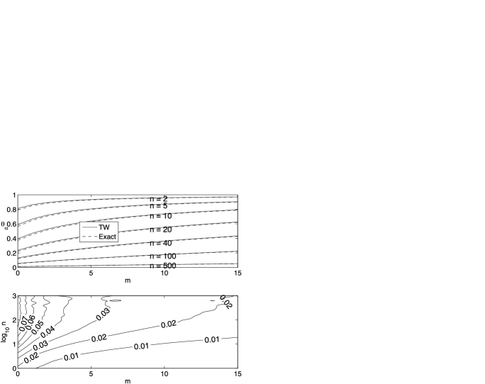
Figure 2: Comparison of exact and approximate 95th percentiles for $\mathsf{s}=2$. Top panel: solid line is the Tracy–Widom approximation $\theta_{\alpha}^{\mathrm{TW}}(2,\mathsf{m},\mathsf{n})$ plotted as a function of $\mathsf{m}$ for values of $\mathsf{n}$ shown. Dashed lines are the exact percentiles $\theta_{\alpha}(2,\mathsf{m},\mathsf{n})$ from Chen’s tables. Bottom panel: Contour plots of relative error $r=(\theta_{\alpha}^{\mathrm{TW}}/\theta_{\alpha})-1$. Horizontal axis is $\mathsf{m}$, vertical axis is $\log_{10}\mathsf{n}$, thus covering the range from $\mathsf{n}=1$ to $1000$.

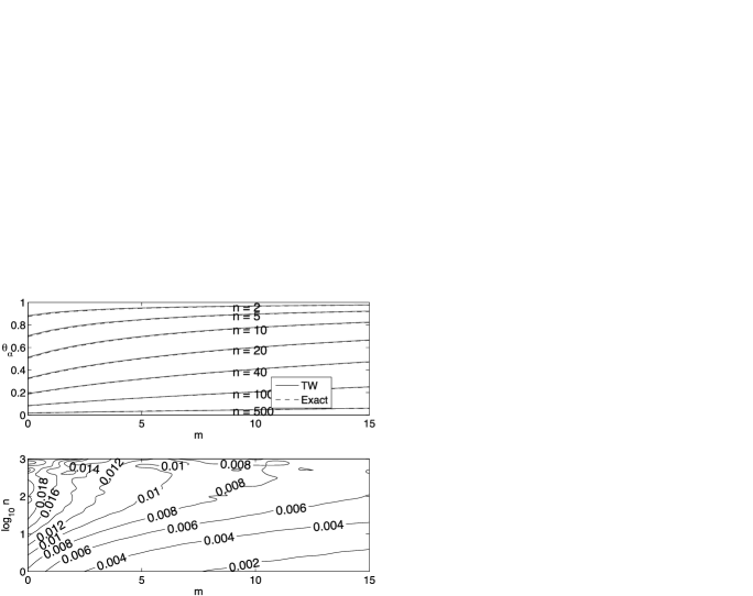
Figure 3: Comparison of exact and approximate 90th percentiles for $\mathsf{s}=4$. Top panel: solid line is the Tracy–Widom approximation $\theta_{\alpha}^{\mathrm{TW}}(4,\mathsf{m},\mathsf{n})$ plotted as a function of $\mathsf{m}$ for values of $\mathsf{n}$ shown. Dashed lines are the exact percentiles $\theta_{\alpha}(4,\mathsf{m},\mathsf{n})$ from Chen’s tables. Bottom panel: Contour plots of relative error $r=(\theta_{\alpha}^{\mathrm{TW}}/\theta_{\alpha})-1$. Horizontal axis is $\mathsf{m}$, vertical axis is $\log_{10}\mathsf{n}$, thus covering the range from $\mathsf{n}=1$ to $1000$.

Work on tables

There has been a large amount of work to prepare tables or charts for the null distribution of the largest root, much of which is reviewed in Chen (2003). We mention contributions by the following: Nanda (1948, 1951); Foster and Rees (1957); Foster (1957, 1958); Pillai (1955, 1956a, 1956b, 1957, 1965, 1967); Pillai and Bantegui (1959); Heck (1960); Krishnaiah (1980); Pillai and Flury (1984); Chen (2002, 2003, 2004a, 2004b).

Because of the dependence on the three parameters, these tables can run up to 25 pages in typical textbooks, such as those of Johnson and Wichern (2002) and Morrison (2005).

Code

Constantine (1963) expresses the c.d.f. of the largest root distribution in terms of a matrix hypergeometric function. Koev and Edelman (2006) have developed efficient algorithms (and a MATLAB package available at http://www-math.mit.edu/~plamen) for the evaluation of such matrix hypergeometric functions using recursion formulas from group representation theory.

Koev (2010) collects useful formulas and explains how to use them and mhg to compute the exact c.d.f. and percentiles for the largest root distribution over a range of values of the “MKB” parameters corresponding to $m,n,p\leq 17$, and $m,n,p\leq 40$ when $n-p$ is odd.

SAS/STAT 9.0 made available an option for computing exact $p$-values using Davis (1972); Pillai and Flury (1984). There is also some stand-alone software described by Lutz (1992, 2000).

2.2 Accuracy of $p$-values

The univariate $F$ bound. We recall the hypothesis that $\mathbf{A}\sim W_{p}(\mathbf{I},m)$ be distributed independently of $\mathbf{B}\sim W_{p}(\mathbf{I},n)$, and the characterization of the largest eigenvalue given by

$$\lambda_{\max}(\mathbf{A}^{-1}\mathbf{B})=\max_{|\mathbf{u}|=1}\frac{\mathbf{u}^{\prime}\mathbf{B}\mathbf{u}}{\mathbf{u}^{\prime}\mathbf{A}\mathbf{u}}.$$ (10)

For fixed $\mathbf{u}$ of unit length, the numerator and denominator are distributed as independent $\chi^{2}_{(n)}$ and $\chi^{2}_{(m)}$ respectively, and so, again for fixed $\mathbf{u}$, the ratio has an $F_{n,m}$ distribution. Consequently, we have the simple bound

$$\frac{m}{n}\lambda_{\max}(\mathbf{A}^{-1}\mathbf{B})>F\sim F_{n,m}.$$

Using the $F_{n,m}$ distribution in place of the actual greatest root law yields a lower bound for the significance level, or $p$-value. We shall see that this bound can be anti-conservative by several orders of magnitude, leading to overstatements of the empirical evidence against the null hypothesis. And furthermore, one can expect that the higher the dimension $p$ of the search space in (10), the worse the bound provided by the $F$ distribution.

The default $p$-value provided in both SAS and R (through package car) uses this unsatisfactory distribution bound.

Table 1 attempts to capture a variety of scenarios within the computational range of Koev’s software.

Column Exact shows a range of significance levels $\alpha$ covering several orders of magnitude. Column Largest Root shows the corresponding quantiles $\theta_{\alpha}$ of the largest root distribution, for the given values of $(\mathsf{s,m,n})$—these are computed using Koev’s MATLAB routine qmaxeigjacobi. Thus, an observed value of $\theta(\mathsf{s,m,n})=\theta_{\alpha}$ would correspond to an exact $p$-value $\alpha$.

The remaining columns compare the Tracy–Widom approximation and the $F$ bound. The $p$-value obtained from the Tracy–Widom approximation is given by

$$P_{\mathrm{TW}}(\theta_{\alpha})=1-F_{1}\bigl{(}\bigl{(}\operatorname{logit}(\theta_{\alpha})-\mu\bigr{)}/\sigma\bigr{)},$$ (11)

where $\mu$ and $\sigma$ are computed from (9).

The $F$ bound on the $p$-value is given by

$$P\bigl{(}\theta(\mathsf{s,m,n})>\theta_{\alpha}\bigr{)}>P_{F}(\theta_{\alpha})=1-F_{\nu_{1},\nu_{2}}\bigl{(}\nu_{2}\theta_{\alpha}/\bigl{(}\nu_{1}(1-\theta_{\alpha})\bigr{)}\bigr{)},$$ (12)

where $\nu_{1}=\mathsf{s}+2\mathsf{m}+1$ and $\nu_{2}=\mathsf{s}+2\mathsf{n}+1$ denote the hypothesis and error degrees of freedom respectively.

The two tables consider $\mathsf{s}=2$ and $6$ variables respectively. The values of $\mathsf{m}=-0.5$ and $5$ correspond to $\mathsf{s}$ and $\mathsf{s}+11$ hypothesis degrees of freedom, while the values of $\mathsf{n}=2$ and $10$ translate to $\mathsf{s}+5$ and $\mathsf{s}+21$ error degrees of freedom respectively.

At the $10\%$ and $5\%$ levels, the Tracy–Widom approximation is within $20\%$ of the true $p$-value at $\mathsf{s}=6$, and within $35\%$ of truth at $\mathsf{s}=2$. The $F$-value is wrong by a factor of four or more at $\mathsf{s}=2$, and by three orders of magnitude at $\mathsf{s}=6$. At smaller significance levels, the Tracy–Widom approximation generally stays within one order of magnitude of the correct $p$-value—except at $\mathsf{(s,m,n)}=(2,-0.5,10)$. The $F$ approximation is off by many orders of magnitude when $\mathsf{s}=6$.

In addition, we note that the Tracy–Widom approximation is conservative in nearly all cases, the exception being for $\theta\geq 0.985$ in the case $\mathsf{(s,m,n)}=(6,-0.5,2)$. In contrast, the $F$ approximation is always [cf. (12)] anti-conservative, often badly so.

In applications one is often concerned only with the general order of magnitude of the $p$-values associated with tests of the various hypotheses that are entertained—not least because the assumptions of the underlying model are at best approximately true. For this purpose, then, it may be argued that the TW approximate $p$-value is often quite adequate over the range of $(\mathsf{s,m,n})$ values. Of course, if $(\mathsf{s,m,n})$ is not too large and greater precision is required, then exact $p$-values can be sought, using, for example, SAS or Koev’s software.

Table 1: Comparison of the Tracy–Widom approximation and $F$ bound for cases with $\mathsf{s}=2$ and $\mathsf{s}=6$ variables

Largest root	Exact	Tracy$\bolds{-}$Widom	F	Largest root	Exact	Tracy$\bolds{-}$Widom	F
$\mathsf{s}=2,\mathsf{m}=-0.5,\mathsf{n}=2$				$\mathsf{s}=6,\mathsf{m}=-0.5,\mathsf{n}=2$
0.663	0.1	0.119	0.0223	0.918	0.1	0.115	2.23e-005
0.737	0.05	0.066	0.00933	0.938	0.05	0.0598	4.99e-006
0.850	0.01	0.0169	0.00131	0.966	0.01	0.0116	1.92e-007
0.881	0.005	0.00927	0.000573	0.973	0.005	0.00545	4.96e-008
0.931	0.001	0.00222	8.49e-005	0.985	0.001	0.000839	2.3e-009
0.968	0.0001	0.000251	5.65e-006	0.993	0.0001	4.35e-005	3.1e-011
0.985	1e-005	2.38e-005	3.81e-007	0.997	1e-005	1.64e-006	4.38e-013
0.993	1e-006	1.89e-006	2.58e-008	0.999	1e-006	NaN	6.33e-015
$\mathsf{s}=2,\mathsf{m}=-0.5,\mathsf{n}=10$				$\mathsf{s}=6,\mathsf{m}=-0.5,\mathsf{n}=10$
0.268	0.1	0.117	0.0278	0.597	0.1	0.11	0.000206
0.318	0.05	0.0669	0.0123	0.633	0.05	0.0577	6.49e-005
0.418	0.01	0.0214	0.00199	0.698	0.01	0.0134	5.46e-006
0.456	0.005	0.0137	0.000919	0.721	0.005	0.00722	1.99e-006
0.533	0.001	0.00522	0.000157	0.766	0.001	0.00172	2.05e-007
0.624	0.0001	0.00146	1.31e-005	0.816	0.0001	0.000223	8.97e-009
0.696	1e-005	0.000443	1.11e-006	0.854	1e-005	2.86e-005	4.29e-010
0.755	1e-006	0.000141	9.59e-008	0.884	1e-006	3.57e-006	2.17e-011
$\mathsf{s}=2,\mathsf{m}=5,\mathsf{n}=10$				$\mathsf{s}=6,\mathsf{m}=5,\mathsf{n}=10$
0.592	0.1	0.112	0.0234	0.757	0.1	0.108	0.000117
0.629	0.05	0.0602	0.0103	0.781	0.05	0.0557	3.63e-005
0.697	0.01	0.0149	0.00164	0.823	0.01	0.0119	2.99e-006
0.721	0.005	0.00827	0.000758	0.837	0.005	0.00606	1.08e-006
0.767	0.001	0.00215	0.000129	0.864	0.001	0.00125	1.1e-007
0.817	0.0001	0.000318	1.07e-005	0.894	0.0001	0.000125	4.75e-009
0.855	1e-005	4.71e-005	9.04e-007	0.917	1e-005	1.17e-005	2.25e-010
0.885	1e-006	6.88e-006	7.79e-008	0.934	1e-006	1.03e-006	1.13e-011

3 Testing for independence of two sets of variables

Let $\mathbf{x}_{1},\ldots,\mathbf{x}_{n}$ be a random sample from $N_{p}(\bolds{\mu},\bolds{\Sigma})$. Partition the variables into two sets with dimensions $p_{1}$ and $p_{2}$ respectively, $p_{1}+p_{2}=p$. Suppose that $\bolds{\Sigma}$ and the sample covariance matrix $\mathbf{S}$ are partitioned correspondingly. We consider testing the null hypothesis of independence of the two sets of variables: $\bolds{\Sigma}_{12}=\mathbf{0}$. The union-intersection test is based on the largest eigenvalue $\lambda_{1}$ of $\mathbf{S}_{22}^{-1}\mathbf{S}_{21}\mathbf{S}_{11}^{-1}\mathbf{S}_{12}$ (Mardia, Kent and Bibby (1979), page 136) and under $H_{0},\lambda_{1}$ has the greatest root distribution $\theta(p_{2},n-1-p_{1},p_{1})$. Mardia, Kent and Bibby (1979) consider an example test of independence of $n=25$ head length and breadth measurements between first sons and second sons, so that $p_{1}=p_{2}=2$. The observed value $\lambda_{1}^{\mathrm{obs}}=0.622$ exceeds the critical value $\theta_{0.05}=0.330$ found by interpolation from the tables. The Tracy–Widom approximation $\theta_{0.05}^{\mathrm{TW}}=0.356$ is found from (6) and serves equally well for rejection of $H_{0}$ in this case.

4 Canonical correlation analysis

Again we have two sets of variables, an $\mathbf{x}$-set with $q$ variables and a $\mathbf{y}$-set with $p$ variables. The goal is to find maximally correlated linear combinations $\eta=\mathbf{a}^{\prime}\mathbf{x}$ and $\phi=\mathbf{b}^{\prime}\mathbf{y}$. We suppose that $(\mathbf{X},\mathbf{Y})$ is a data matrix of $n$ samples (rows) on $q+p$ variables (columns) such that each row is an independent draw from $N_{p+q}(\bolds{\mu},\bolds{\Sigma})$. Again let $\mathbf{S}$ be the sample covariance matrix, assumed partitioned $\mathbf{S}=\bigl{(}{\mathbf{S}_{11}\atop\mathbf{S}_{21}}\enskip{\mathbf{S}_{12}\atop\mathbf{S}_{22}}\bigr{)}$. The sample squared canonical correlations $(r_{i}^{2})$ for $i=1,\ldots,k=\min(p,q)$ are found as the eigenvalues of $\mathbf{M}_{2}=\mathbf{S}_{22}^{-1}\mathbf{S}_{21}\mathbf{S}_{11}^{-1}\mathbf{S}_{12}$ [Mardia, Kent and Bibby (1979), Sections 10.2.1 and 10.2.2]. The population squared canonical correlations $\rho_{i}^{2}$ are, in turn, the eigenvalues of $\bolds{\Sigma}_{22}^{-1}\bolds{\Sigma}_{21}\bolds{\Sigma}_{11}^{-1}\bolds{\Sigma}_{12}$. In both cases, we assume that the correlations are arranged in decreasing order. The test of the null hypothesis of zero correlation, $H_{0}\dvtx\rho_{1}=\cdots=\rho_{k}=0$, is based on the largest eigenvalue $r_{1}^{2}$ of $\mathbf{M}_{2}$. Under $H_{0}$, it is known that $r_{1}^{2}$ has the $\theta(p,n-q-1,q)$ distribution, so that the Tracy–Widom approximation can be applied.

Nonnull cases—a conservative test

Often it may be apparent that the first $k$ canonical correlations are nonzero and the main interest focuses on the significance of $r_{k+1}^{2},r_{k+2}^{2}$, etc. We let $H_{s}$ denote the null hypothesis that $\rho_{s+1}=\cdots=\rho_{p}=0$, and write $\mathcal{L}(r_{k}|p,q,n;\bolds{\Sigma})$ for the distribution of the $r$th c.c. under population covariance matrix $\bolds{\Sigma}$. When the covariance matrix $\bolds{\Sigma}\in H_{s}$, the $(s+1)$st canonical correlation is stochastically smaller than the largest canonical correlation in a related null model:

Lemma 1

If $\bolds{\Sigma}\in H_{s}$, then

$$\mathcal{L}(r_{s+1}|p,q,n;\bolds{\Sigma})\stackrel{{\scriptstyle st}}{{<}}\mathcal{L}(r_{1}|p,q-s,n;\mathbf{I}).$$

This nonasymptotic result follows from interlacing properties of the singular value decomposition (Appendix). Since $\mathcal{L}(r_{1}^{2}|p,q-s,n;\mathbf{I})$ is given by the null distribution $\theta(p,n+s-q-1,q-s)$, we may use the latter to provide a conservative $p$-value for testing $H_{s}$. In turn, the $p$-value for $\theta(p,n+s-q-1,q-s)$ can be numerically approximated as in (6) using the Tracy–Widom distribution.

Example

Waugh (1942) gave perhaps the first significant illustration of CCA using data on $n=138$ samples of Canadian Hard Red Spring wheat and the flour made from each of these samples. The aim was to seek highly correlated indices $\mathbf{a}^{\prime}\mathbf{x}$ of wheat quality and $\mathbf{b}^{\prime}\mathbf{y}$ of flour quality, since a well correlated grading of raw (wheat) and finished (flour) products was believed to promote fair pricing of each. In all, $q=5$ wheat characteristics—kernel texture, test weight, damaged kernels, foreign material, crude protein in wheat—and $p=4$ flour characteristics—wheat per bushel of flour, ash in flour, crude protein in flour, gluten quality index—were measured. The resulting squared canonical correlations were $(r_{1}^{2},r_{2}^{2},r_{3}^{2},r_{4}^{2})=(0.923,0.554,\break 0.056,0.008)$. The leading correlation would seem clearly significant and, indeed, from our approximate formula (6), $\theta_{0.99}^{\mathrm{TW}}=0.184$.

To assess the second correlation $r_{2}$, we appeal to the conservative test discussed above based on the null distribution with $q-1=4,p=4$ and $n=138$. The Tracy–Widom approximation $\theta_{0.99}^{\mathrm{TW}}\approx\mu+2.023\sigma\doteq 0.166\ll 0.554$, which strongly suggests that this second correlation is significant as well.

Marginal histograms naturally reveal some departures from symmetric Gaussian tails, but they do not seem extreme enough to invalidate the conclusions, which are also confirmed by permutation tests.

5 Tests of common means or variances

5.1 Equality of means for common covariance

Suppose that we have $k$ populations with independent data matrices $\mathbf{X}_{i}$ consisting of $n_{i}$ observations drawn from an $N_{p}(\bolds{\mu}_{i},\bolds{\Sigma}_{i})$ and put $n=\sum n_{i}$. This is the one-way multivariate analysis of variance illustrated in Example 1.1. For testing the null hypothesis of equality of means $H_{0}\dvtx\bolds{\mu}_{1}=\cdots=\bolds{\mu}_{k}$, we form, for each population, the sample mean $\bar{\mathbf{x}}_{i}$ and covariance matrix $\mathbf{S}_{i}$, normalized so that $n_{i}\mathbf{S}_{i}\sim W_{p}(\bolds{\Sigma},n_{i}-1)$. The basic quantities are the within groups sum of squares $\mathbf{W}=\sum n_{i}\mathbf{S}_{i}\sim W_{p}(\bolds{\Sigma},n-k)$ and the between group sum of squares $\mathbf{B}=\sum n_{i}(\bar{\mathbf{x}}_{i}-\bar{\mathbf{x}})(\bar{\mathbf{x}}_{i}-\bar{\mathbf{x}})^{\prime}\sim W_{p}(\bolds{\Sigma},k-1)$ under $H_{0}$, independently of $\mathbf{W}$. The union-intersection test of $H_{0}$ uses the largest root of $\mathbf{W}^{-1}\mathbf{B}$ or, equivalently, that of $(\mathbf{W}+\mathbf{B})^{-1}\mathbf{B}$, and the latter has, under $H_{0}$, the $\theta(p,n-k,k-1)$ distribution.

5.2 Equality of covariance matrices

Suppose that independent samples from two normal distributions $N_{p}(\bolds{\mu}_{1},\bolds{\Sigma}_{1})$ and $N_{p}(\bolds{\mu}_{2},\bolds{\Sigma}_{2})$ lead to covariance estimates $\mathbf{S}_{i}$ which are independent and Wishart distributed on $n_{i}$ degrees of freedom: $n_{i}\mathbf{S}_{i}\sim W_{p}(n_{i},\bolds{\Sigma}_{i})$ for $i=1,2$. Then the largest root test of the null hypothesis $H_{0}\dvtx\bolds{\Sigma}_{1}=\bolds{\Sigma}_{2}$ is based on the largest eigenvalue $\theta$ of $(n_{1}\mathbf{S}_{1}+n_{2}\mathbf{S}_{2})^{-1}n_{2}\mathbf{S}_{2}$, which under $H_{0}$ has the $\theta(p,n_{1},n_{2})$ distribution Muirhead (1982), page 332.

6 Multivariate linear model

The multivariate linear model blends ideas well known from the univariate setting with new elements introduced by correlated multiple responses. In view of the breadth of models covered, and the variety of notation in the literature and in the software, we review the setting in a little more detail, beginning with the familiar model for a single response

$$\mathbf{y}=\mathbf{X}\bolds{\beta}+\mathbf{u}.$$

Here $\mathbf{y}$ is an $n\times 1$ column vector of observations on a response variable, $\mathbf{X}$ is an $n\times q$ model matrix, and $\mathbf{u}$ is an $n\times 1$ column vector of errors, assumed here to be independent and identically distributed as $N(0,\sigma^{2})$. The $q\times 1$ vector $\bolds{\beta}$ of unknown parameters has the least squares estimate—when $\mathbf{X}$ has full rank—given by

$$\hat{\bolds{\beta}}=(\mathbf{X}^{\prime}\mathbf{X})^{-1}\mathbf{X}^{\prime}\mathbf{y}.$$

The error sum of squares $SS_{E}=(\mathbf{y-X\hat{\bolds{\beta}}})^{\prime}(\mathbf{y-X\hat{\bolds{\beta}}})=\mathbf{y^{\prime}Py}$, where $\mathbf{P}$ denotes orthogonal projection onto the subspace orthogonal to the columns of $\mathbf{X}$, it has rank $n-q$, and so $SS_{E}\sim\chi^{2}_{(n-q)}$.

Consider the linear hypothesis $H_{0}\dvtx\mathbf{C}_{1}\bolds{\beta}=0$, where $\mathbf{C}_{1}$ is a $g\times q$ matrix of rank $g$. In the simplest example, $\mathbf{C}_{1}=[\mathbf{I}_{g}\ \mathbf{0}]$ extracts the first $g$ elements of $\bolds{\beta}$; more generally, the rows of $\mathbf{C}_{1}$ are often contrasts among the components of $\bolds{\beta}$. To describe the standard $F$-test of $H_{0}$, let $\mathbf{C}_{2}$ be any $(q-g)\times q$ matrix such that $\mathbf{C}={\mathbf{C}_{1}\choose\mathbf{C}_{2}}$ becomes an invertible $q\times q$ matrix. We may then write

$$\mathbf{X}\bolds{\beta}=\bigl{[}\matrix{\mathbf{XC}^{(1)}&\mathbf{XC}^{(2)}}\bigr{]}\pmatrix{\mathbf{C}_{1}\bolds{\beta}\cr\mathbf{C}_{2}\bolds{\beta}},$$

where we have partitioned $\mathbf{C}^{-1}=[\mathbf{C}^{(1)}\ \mathbf{C}^{(2)}]$ into blocks with $g$ and $q-g$ columns respectively.

Let $\mathbf{P}_{1}$ denote the orthogonal projection onto the subspace orthogonal to the columns of $\mathbf{XC}^{(2)}$. We have the sum of squares decomposition

$$\mathbf{y^{\prime}P}_{1}\mathbf{y}=\mathbf{y^{\prime}Py}+\mathbf{y^{\prime}}(\mathbf{P}_{1}-\mathbf{P})\mathbf{y}$$

and the hypothesis sum of squares for testing $H_{0}:\mathbf{C}_{1}\bolds{\beta}=0$ is given by $SS_{H}=\mathbf{y^{\prime}P}_{2}\mathbf{y}$, with $\mathbf{P}_{2}=\mathbf{P}_{1}-\mathbf{P}$. The projection $\mathbf{P}_{2}$ has rank $g$ and so under $H_{0}$, $SS_{H}\sim\chi^{2}_{(g)}$. The projections $\mathbf{P}$ and $\mathbf{P}_{2}$ are orthogonal and so the sums of squares have independent chi-squared distributions, and under $H_{0}$ the traditional $F$-statistic

$$F=\frac{SS_{H}/g}{SS_{E}/(n-q)}\sim F_{g,n-q}.$$

Explicit expressions for the sums of squares are given by

$$SS_{E} = \mathbf{y^{\prime}\bigl{(}I-X(X^{\prime}X)^{-1}X^{\prime}\bigr{)}y},$$

$$SS_{H} = (\mathbf{C}_{1}\hat{\bolds{\beta}})^{\prime}[\mathbf{C}_{1}\mathbf{(X^{\prime}X)^{-1}}\mathbf{C}_{1}^{\prime}]^{-1}\mathbf{C}_{1}\hat{\bolds{\beta}}.$$

In the multivariate linear model,

$$\mathbf{Y}=\mathbf{X}\mathbf{B}+\mathbf{U},$$

the single response $\mathbf{y}$ is replaced by $p$ response vectors, organized as columns of the $n\times p$ matrix $\mathbf{Y}$. The model (or design) matrix $\mathbf{X}$ remains the same for each response; however, there are separate vectors of unknown coefficients and errors for each response; these are organized into a $q\times p$ matrix $\mathbf{B}$ of regression coefficients and an $n\times p$ matrix $\mathbf{E}$ of errors. The multivariate aspect of the model is the assumption that the rows of $\mathbf{U}$ are indepedent, with multivariate normal distribution having mean $\mathbf{0}$ and common covariance matrix $\bolds{\Sigma}$. Thus, $\mathbf{U}$ is a normal data matrix of $n$ samples from $N_{p}(\mathbf{0},\bolds{\Sigma})$. Assuming for now that the model matrix $\mathbf{X}$ has full rank, the least squares estimator

$$\hat{\mathbf{B}}=\mathbf{(X^{\prime}X)^{-1}X^{\prime}Y}.$$

The linear hypothesis becomes

$$H_{0}\dvtx\mathbf{C}_{1}\mathbf{B}=\mathbf{0}.$$

The sums of squares of the univariate case are replaced by hypothesis and error sums of squares and products matrices:

$$E = \mathbf{Y^{\prime}PY}=\mathbf{Y^{\prime}\bigl{(}I-X(X^{\prime}X)^{-1}X^{\prime}\bigr{)}Y},$$

$$H = \mathbf{Y^{\prime}P}_{2}\mathbf{Y}=(\mathbf{C}_{1}\hat{\mathbf{B}})^{\prime}[\mathbf{C}_{1}\mathbf{(X^{\prime}X)^{-1}}\mathbf{C}_{1}^{\prime}]^{-1}\mathbf{C}_{1}\hat{\mathbf{B}},$$

in which the univariate vectors $\mathbf{y}$ and $\hat{\bolds{\beta}}$ are simply replaced by their multivariate analogs $\mathbf{Y}$ and $\hat{\mathbf{B}}$. It follows that $\mathbf{E}\sim W_{p}(\bolds{\Sigma},n-q)$ and that under $H_{0}$, $\mathbf{H}\sim W_{p}(\bolds{\Sigma},g)$; furthermore, $\mathbf{E}$ and $\mathbf{H}$ are independent. Generalizations of the $F$-test are obtained from the eigenvalues $(\lambda_{i})$ of the matrix $\mathbf{E}^{-1}\mathbf{H}$ or, equivalently, the eigenvalues $\theta_{i}$ of $(\mathbf{H+E})^{-1}\mathbf{H}$.

Thus, under the null hypothesis $\mathbf{C}_{1}\mathbf{B}=0$, Roy’s maximum root statistic $\theta_{1}$ has null distribution

$$\theta_{1}\sim\theta(p,n-q,g),\qquad\mbox{where}$$

$$\qquad p=\mbox{dimension},\qquad g=\operatorname{rank}(\mathbf{C}_{1}),$$ (14)

$$\hskip 1.0pt\qquad q=\operatorname{rank}(\mathbf{X}),\hskip 10.0pt\qquad n=\mbox{sample size}.$$

Two extensions

(a) $X$ not of full rank. This situation routinely occurs when redundant parameterizations are used, for example, when dealing with factors in analysis of variance models. One approach (e.g., MKB, Section 6.4) is to rearrange the columns of $\mathbf{X}$ and partition $\mathbf{X}=[\mathbf{X}_{1}\ \mathbf{X}_{2}]$ so that $\mathbf{X}_{1}$ has full rank. We must also assume that the matrix $\mathbf{C}_{1}$ is testable in the sense that, as a function of $\mathbf{B}$, $\mathbf{XB}=\mathbf{0}$ implies $\mathbf{C}_{1}\mathbf{B}=\mathbf{0}$. In such cases, if we partition $\mathbf{C}_{1}=[\mathbf{C}_{11}\ \mathbf{C}_{12}]$ conformally with $\mathbf{X}$, then $\mathbf{C}_{12}=\mathbf{C}_{11}(\mathbf{X}^{\prime}_{1}\mathbf{X}_{1})^{-1}\mathbf{X}^{\prime}_{1}\mathbf{X}_{2}$ is determined from $\mathbf{C}_{11}$.

With these assumptions, we use $\mathbf{X}_{1}$ and $\mathbf{C}_{11}$ in (6) and (6) in place of $\mathbf{X}$ and $\mathbf{C}_{1}$.

(b) Intra-subject hypotheses. A straightforward extension is possible in order to test null hypotheses of the form

$$\mathbf{C}_{1}\mathbf{B}\mathbf{M}_{1}=0,$$

where $\textbf{M}_{1}$ is $p\times r$ of rank $r$. The columns of $\mathbf{M}_{1}$ capture particular linear combinations of the dependent variables—for an example, see, e.g., Morrison (2005), Chapter 3.6.

We simply consider a modified linear model

$$\mathbf{YM}_{1}=\mathbf{XBM}_{1}+\mathbf{UM}_{1}.$$

An important point is that the rows of $\mathbf{UM}_{1}$ are still independent, now distributed as $N_{p}(\mathbf{0},\mathbf{M}^{\prime}_{1}\bolds{\Sigma}\mathbf{M})$. So we may simply apply the above analysis, replacing $\mathbf{Y},\mathbf{U}$ and $\mathbf{B}$ by $\mathbf{YM}_{1}$, $\mathbf{UM}_{1}$ and $\mathbf{BM}_{1}$ respectively. In particular, the greatest root statistic now has null distribution given by

$$\theta_{1}\sim\theta(r,n-q,g).$$

Linear hypotheses in SAS

Analyses involving the four multivariate tests are provided in a number of SAS routines, such as GLM and CANCORR. The parameterization used here can be translated into that used in SAS by means of the documentation given in the SAS/STAT Users Guide—we refer to the section on Multivariate Tests in version 9.1, page 48 ff. The linear hypotheses correspond to MKB notation via

MKB	SAS
$\mathbf{C}_{1}$	$\mathbf{L}$
$\mathbf{B}$	$\bolds{\beta}$
$\mathbf{M}_{1}$	$\mathbf{M}$

while the parameters of the greatest root distribution are given by

	MKB		SAS
dimension	$r$	$\operatorname{rank}(\textbf{M}_{1})$	$\operatorname{rank}(\mathbf{M})$	$\mathsf{p}$
hypothesis	$g$	$\operatorname{rank}(\mathbf{C}_{1})$	$\operatorname{rank}(\mathbf{L})$	$\mathsf{q}$
error	$n-q$			$\mathsf{v}$

.

(Note: we use sans serif font for the SAS parameters!) Finally, the SAS printouts use the following parameters:

$$\mathsf{s} = \mathsf{p}\wedge\mathsf{q},$$

$$\mathsf{m} = (|\mathsf{p}-\mathsf{q}|-1)/2,$$

$$\mathsf{n} = (\mathsf{v}-\mathsf{p}-1)/2.$$

7 Concluding discussion

We have described the Tracy–Widom approximation to the null distribution for the largest root test for a variety of classical multivariate procedures. These procedures exhibit varying degrees of sensitivity to the assumption of normality, independence etc. Documenting the sensitivity/robustness of the T–W approximation is clearly an important issue for further work. Two brief remarks can be made. In the corresponding single Wishart setting [e.g., Johnstone (2001)], the largest eigenvalue can be shown, under the null distribution, to still have the T–W limit if the original data have “light tails” (i.e., sub-Gaussian) [see Soshnikov (2002); Péché (2009)]. In the double Wishart settings, simulations for canonical correlation analysis with $n=100$ samples on $q=20$ and $p=10$ variables, each following i.i.d. $t_{(5)}$ or i.i.d. random sign distributions, showed that the T–W distribution for the leading correlation $r_{1}^{2}$ still holds in the central 99% of the distribution.

Appendix: Proof of lemma

If $\bolds{\Sigma}\in H_{s}$, there are at most $s$ nonzero canonical correlations, and we may suppose without loss of generality that the $q$ $\mathbf{x}$-variables have been transformed so that only the last $s$ of them have any correlation with $\mathbf{Y}$. We employ the singular value decomposition (SVD) description of CCA, cf. Golub and Van Loan (1996), Section 12.4.3. Using QR decompositions, write

$$\mathbf{X}=Q_{X}R_{X},\qquad\mathbf{Y}=Q_{Y}R_{Y}.$$

Let $C=Q_{X}^{T}Q_{Y}$ and form the SVD $C=URV^{T}$. Then the diagonal elements $r_{1}\geq r_{2}\geq\cdots\geq r_{\min(p,q)}$ of $R$ contain the sample canonical correlations.

Now consider the reduced $n\times(q-s)$ matrix $\mathbf{X}^{-}$ obtained by dropping the last $s$ columns from $\mathbf{X}$. Form the QR decomposition $\mathbf{X}^{-}=Q_{X^{-}}R_{X^{-}}$. From the nature of the decomposition, we have $Q_{X}=[Q_{X^{-}}\ Q^{+}]$, that is, $Q_{X^{-}}$ represents the first $q-s$ columns of $Q_{X}$. Consequently, $C_{-}=Q_{X^{-}}^{T}Q_{Y}$ forms the first $q-s$ rows of $C$. Our lemma now follows from the interlacing property of singular values [e.g., Golub and Van Loan (1996), Corollary 8.6.3].

$$\sigma_{s+1}(C)\leq\sigma_{1}(C_{-}).$$

Indeed, our earlier discussion implies that $\mathbf{X}^{-}$ and $\mathbf{Y}$ are independent, and so $\sigma_{1}(C_{-})$ has the null distribution $\mathcal{L}(r_{1}|p,q-s,n;\mathbf{I})$.

References

- Anderson (2003) Anderson, T. W. (2003). An Introduction to Multivariate Statistical Analysis, 3rd ed. Wiley, Hoboken, NJ. \MR1990662
- Andrews and Herzberg (1985) Andrews, D. F. and Herzberg, A. M. (1985). Data. Springer, New York.
- Chen (2002) Chen, W. W. (2002). Some new tables of the largest root of a matrix in multivariate analysis: A computer approach from 2 to 6. Presented at the 2002 American Statistical Association.
- Chen (2003) Chen, W. W. (2003). Table for upper percentage points of the largest root of a determinantal equation with five roots. InterStat (5). Available at interstat.statjournals.net.
- Chen (2004a) Chen, W. W. (2004a). The new table for upper percentage points of the largest root of a determinantal equation with seven roots. InterStat (1). Available at interstat.statjournals.net.
- Chen (2004b) Chen, W. W. (2004b). Some new tables for the upper probability points of the largest root of a determinantal equation with seven and eight roots. In Special Studies in Federal Tax Statistics. Statistics of Income Division, Internal Revenue Service (J. Dalton and B. Kilss, eds.) 113–116.
- Constantine (1963) Constantine, A. G. (1963). Some non-central distribution problems in multivariate analysis. Ann. Math. Statist. 34 1270–1285. \MR0181056
- Davis (1972) Davis, A. W. (1972). On the marginal distributions of the latent roots of the multivariate beta matrix. Ann. Math. Statist. 43 1664–1670. \MR0343465
- Foster (1957) Foster, F. G. (1957). Upper percentage points of the generalized Beta distribution. II. Biometrika 44 441–453. \MR0090199
- Foster (1958) Foster, F. G. (1958). Upper percentage points of the generalized Beta distribution. III. Biometrika 45 492–503. \MR0100366
- Foster and Rees (1957) Foster, F. G. and Rees, D. H. (1957). Upper percentage points of the generalized Beta distribution. I. Biometrika 44 237–247. \MR0086462
- Golub and Van Loan (1996) Golub, G. H. and Van Loan, C. F. (1996). Matrix Computations, 3rd ed. Johns Hopkins Univ. Press, Baltimore. \MR1417720
- Heck (1960) Heck, D. L. (1960). Charts of some upper percentage points of the distribution of the largest characteristic root. Ann. Math. Statist. 31 625–642. \MR0119301
- Johnson and Wichern (2002) Johnson, R. A. and Wichern, D. W. (2002). Applied Multivariate Statistical Analysis, 6th ed. Pearson Prentice Hall, Upper Saddle River, NJ.
- Johnstone (2001) Johnstone, I. M. (2001). On the distribution of the largest eigenvalue in principal components analysis. Ann. Statist. 29 295–327. \MR1863961
- Johnstone (2008) Johnstone, I. M. (2008). Multivariate analysis and Jacobi ensembles: Largest eigenvalue, Tracy–Widom limits and rates of convergence. Ann. Statist. 36 2638–2716. \MR2485010
- Johnstone and Chen (2007) Johnstone, I. M. and Chen, W. W. (2007). Finite sample accuracy of Tracy–Widom approximation for multivariate analysis. In 2007 JSM Proceedings 1161–1166. Amer. Statist. Assoc., Alexandria, VA.
- Johnstone et al. (2010) Johnstone, I. M., Ma, Z., Perry, P. O. and Shahram, M. (2010). RMTstat: Distributions, statistics and tests derived from random matrix theory. Manuscript in preparation.
- Koev (2010) Koev, P. (2010). Computing multivariate statistics. Manuscript in preparation.
- Koev and Edelman (2006) Koev, P. and Edelman, A. (2006). The efficient evaluation of the hypergeometric function of a matrix argument. Math. Comp. 75 833–846 (electronic). \MR2196994
- Krishnaiah (1980) Krishnaiah, P. R. (1980). Computations of some multivariate distributions. In Handbook of Statistics, Volume 1—Analysis of Variance (P. R. Krishnaiah, ed.) 745–971. North-Holland, Amsterdam.
- Lutz (1992) Lutz, J. G. (1992). A Turbo Pascal unit for approximating the cumulative distribution function of Roy’s largest root criterion. Educational and Psychological Measurement 52 899–904.
- Lutz (2000) Lutz, J. G. (2000). Roy table: A program for generating tables of critical values for Roy’s largest root criterion. Educational and Psychological Measurement 60 644–647.
- Mardia, Kent and Bibby (1979) Mardia, K. V., Kent, J. T. and Bibby, J. M. (1979). Multivariate Analysis. Academic Press, London. \MR0560319
- Morrison (2005) Morrison, D. F. (2005). Multivariate Statistical Methods, 4th ed. Thomson, Belmont, CA.
- Muirhead (1982) Muirhead, R. J. (1982). Aspects of Multivariate Statistical Theory. Wiley, New York. \MR0652932
- Nanda (1948) Nanda, D. N. (1948). Distribution of a root of a determinantal equation. Ann. Math. Statist. 19 47–57. \MR0024106
- Nanda (1951) Nanda, D. N. (1951). Probability distribution tables of the largest root of a determinantal equation with two roots. J. Indian Soc. Agricultural Statist. 3 175–177. \MR0044788
- Péché (2009) Péché, S. (2009). Universality results for largest eigenvalues of some sample covariance matrices ensembles. Probab. Theory Related Fields 143 481–516.
- Pillai (1955) Pillai, K. C. S. (1955). Some new test criteria in multivariate analysis. Ann. Math. Statist. 26 117–121. \MR0067429
- Pillai (1956a) Pillai, K. C. S. (1956a). On the distribution of the largest or smallest root of a matrix in multivariate analysis. Biometrika 43 122–127. \MR0077052
- Pillai (1956b) Pillai, K. C. S. (1956b). Some results useful in multivariate analysis. Ann. Math. Statist. 27 1106–1114. \MR0081852
- Pillai (1957) Pillai, K. C. S. (1957). Concise Tables for Statisticians. The Statistical Center, Univ. of the Philippines, Manila.
- Pillai (1965) Pillai, K. C. S. (1965). On the distribution of the largest characteristic root of a matrix in multivariate analysis. Biometrika 52 405–414. \MR0205391
- Pillai (1967) Pillai, K. C. S. (1967). Upper percentage points of the largest root of a matrix in multivariate analysis. Biometrika 54 189–194. \MR0215433
- Pillai and Bantegui (1959) Pillai, K. C. S. and Bantegui, C. G. (1959). On the distribution of the largest of six roots of a matrix in multivariate analysis. Biometrika 46 237–240. \MR0102152
- Pillai and Flury (1984) Pillai, K. C. S. and Flury, B. N. (1984). Percentage points of the largest characteristic root of the multivariate beta matrix. Commun. Statist. Part A 13 2199–2237. \MR0754832
- Rencher (2002) Rencher, A. C. (2002). Methods of Multivariate Analysis, 2nd ed. Wiley, New York. \MR1885894
- Soshnikov (2002) Soshnikov, A. (2002). A note on universality of the distribution of the largest eigenvalues in certain classes of sample covariance matrices. J. Statist. Phys. 108 1033–1056. \MR1933444
- Tracy and Widom (1996) Tracy, C. A. and Widom, H. (1996). On orthogonal and symplectic matrix ensembles. Commun. Math. Phys. 177 727–754. \MR1385083
- Waugh (1942) Waugh, F. V. (1942). Regressions between sets of variables. Econometrica 10 290–310.