Simultaneous Event Execution in
Heterogeneous Wireless Sensor Networks

Abstract

We present a synchronization algorithm to let nodes in a sensor network simultaneously execute a task at a given point in time. In contrast to other time synchronization algorithms we do not provide a global time basis that is shared on all nodes. Instead, any node in the network can spontaneously initiate a process that allows the simultaneous execution of arbitrary tasks. We show that our approach is beneficial in scenarios where a global time is not needed, as it requires little communication compared with other time synchronization algorithms.

We also show that our algorithm works in heterogeneous systems where the hardware provides highly varying clock accuracy. Moreover, heterogeneity does not only affect the hardware, but also the communication channels. We deal with different connection types—from highly unreliable and fluctuating wireless channels to reliable and fast wired connections.

Keywords:

Sensor Networks, Time Synchronization, Simulatenous Events, Clock Drift, Heterogeneity.

I Introduction

When dealing with algorithms for sensor networks, time synchronization is an important factor. For many kinds of application areas it is essential to have a common global time basis. This can be required due to the need for putting certain events within the network in a chronological order, to execute tasks synchronously, or for clock synchronization in time division multiple access (TDMA) based media access layer (MAC) protocols.

While there are already standards for ordinary networks available, such as the Network Time Protocol (NTP) or Precision Time Protocol (PTP), it is still a challenging task for sensor networks. This is due to several reasons. First, we mainly have wireless communication in sensor networks, and thus a higher amount of unreliability and fluctuation. Second, we must deal with energy constraints. The nodes may be operated with batteries, and hence they are not able to exchange messages frequently over a long period of time. Third, because of low hardware costs the nodes may have a high clock drift—that is, clocks run at a slightly different speed, and so they drift apart even if started at exactly the same time.

There have already been many algorithms developed that deal with these issues. However, there are application scenarios where a consequent time synchronization, with all nodes sharing the same time basis is not needed and would produce too much overhead. For example, if the nodes only need to start a common task at a certain point in time, but do not need any common time basis apart from that, it is possible to use much simpler algorithms. So the network can stay unsynchronized most of the time, but only collaborate shortly before the designated event.

An application for such a system is collaborative sensing of highly dynamic effects. For instance, to locate the source of an audio signal, it is necessary to collect synchronized readings from the sensor network. An initiator node would then start the process so that every node measures the local volume at the very same point in time. The resulting map can then be used to determine the source of the signal. It is obviously crucial that all nodes collect their data at a synchronized point, yet it is not necessary to keep the network synchronous at all times. Another example is simultaneous output, e.g., the playback of music by a sensor network where each node is equipped with a speaker. Here, the sensors must start the playback at a particular time, but any synchronization before the event is not needed.

However, even such a simplification of the requirements may lead to a goal that is hard to achieve. This is especially the case when dealing with heterogeneity in sensor networks. There may be very different kinds of hardware platforms used. Thus, there is a high variance in clock drift among the used architectures. Some platforms may be equipped with very accurate clocks, whereas others provide only very course ones. Moreover, the nodes may communicate over different communication channels—from 2.4 GHz IEEE 802.15.4 over the 868 MHz band to wired Ethernet or even SPI or RS232.

This paper presents an algorithm that deals with the above described issues. First, our algorithm provides a spontaneous, on-demand synchronization mechanism. That means, at an arbitrary point in time, any node in the sensor network is able to act as a master and initiate a synchronization process. The exclusive goal of this process is that all participating nodes can start a task at the same point in time, relative to a start signal from the master. Hence, the nodes do not need a global time basis, and thus messages required for continuous synchronization are completely avoided.

We also address interference issues in our algorithm. To avoid all nodes sending replies to the master at the same time, causing interference in a broadcast medium, the algorithm needs only two participants: one master and one slave. The other nodes in communication range merely overhear the communication without sending any message, but are still able to join in the synchronization event execution. This leads to a considerable reduction of energy consumption and interference.

Second, our algorithm can deal with both heterogeneous networks and hierarchical structures. The former enables the use of different hardware platforms, whereby especially various clock accuracies were taken into account. The latter enables the possibility of building a layered structure of participants. This can be, in the simplest topology, a wireless multihop connection to nodes that can not be directly reached by the master. But it can also be a wired connection between two nodes of completely different hardware platforms.

We show that our approach works accurately with different hardware platforms. Therefore we chose two architectures with different capabilities: One more powerful sensor node that runs quite complicated algorithms, and a very restricted one with supremely limited code space and an inaccurate clock. There are also different communication channels available. Some of the nodes communicate via their radio, whereas others are connected via a wired connection and communicate over SPI.

The next section describes the related work that has already been done in this context. Section III presents our algorithm in detail, followed by the experimental results. Section V concludes this paper.

II Related Work

Time synchronization has been an issue in distributed systems for long time now. Thus an abundance of algorithms is already available [1, 2, 3]. Many of them are unsuitable for wireless sensor networks, as they rely on stable communication, complex calculations, or high clock accuracy.

The remaining algorithms can be categorized roughly by the following properties:

• Relative synchronization calculates the drift between the clocks of two nodes, instead of adjusting them to a central time source.

• Passive nodes perform synchronization without ever communicating themselves, they merely listen to the communicating of others.

• Event-triggered synchronization proceeds only on demand, while continuous synchronization keeps the clocks aligned at all times.

The Reference-Broadcast Synchronization (RBS) [4] is a very common approach. It leads to accurate results and can be event based, but it does not allow for passive nodes. Every pair of nodes has to exchange messages containing their local timestamps at the reception of broadcast signal in order to synchronize. This leads to a high communication rate during the synchronization process, thus increased power consumption and risk of collisions.

An improvement concerning performance is the Timing-sync Protocol for Sensor Networks (TPSN) [5]. It builds a hierarchical structure based on distances to one or more root nodes. Afterwards, every node at distance $d$ to the root synchronizes with a node at distance $d-1$.

Our algorithm is neither similar to RBS nor TPSN. It employs a broadcast element like RBS and a (dynamically changing) hierarchical master-slave structure as in TPSN. Additionally it allows for passive slaves within communication range of the root, which are synchronized without sending any message.

Another active synchronization algorithm is TinySync [6]. It calculates clock drift by exchanging time stamps of two nodes and resolving the linear correlation. Though it allows two nodes to run synchronized for a longer period, it has to perform complex computations and requires storage of many data points. These two disadvantages make it inappropriate for systems with less computing and storage capacity.

TSync [7] allows for passive slaves. It uses one or more reference nodes to broadcast a certain beacon and the local timestamp, when sending it. A selected child node sends its own local timestamp at reception and the current one back. Therefore it is possible for the reference node to calculate the propagation time and the clock offset of the child. Indeed this algorithm is very similar to our approach. Unlike our approach, it does not calculate the clock drift and therefore has to be run periodically.

We already presented a preceding model of our algorithm in [8]. While the fundamental design of the algorithm has not changed, we optimized the synchronization process and obtained noticeably better results than in the previous work. The enhancements concerned particularly the capability of dealing with an implementation in application layer, but also a better adaptation to heterogeneous networks.

III Algorithm

In contrast to other time synchronization algorithms, we do not provide a global time basis on all nodes. Instead, our algorithm allows any node in the network to spontaneously start a synchronous execution of arbitrary tasks. Following this approach, there is no need for sending periodic messages, and thus we achieve a remarkable reduction of energy consumption in scenarios where a global time is not needed.

We assume that any node in the network is allowed to initiate a synchronization process. If so, the self-proclaimed master selects an arbitrary node in communication range to start the synchronization. The slave then obtains two values based on the message exchange: propagation time of the message, and clock drift with respect to the master’s clock.

While the master and the slave calculate the required values, every node in communication range of the master can determine the same values for itself only by listening to the master’s packets.

After that, each node then does the same procedure for its unsynchronized neighbors, which are nodes outside the communication range of the master. Finally, each node participating in the synchronization process knows both the message propagation time and clock drift to its predecessor. Then, the master broadcasts a message with the given time span after which the nodes shall start their execution. Each of these nodes is then able to calculate its local waiting time. In the following, the different phases are described in detail.

III-A Active Synchronization

The active synchronization is done between a master and a slave, whereby the slave is only supposed to calculate its own clock drift relative to the master, and to obtain the propagation time of a message.

The whole process needs only five messages, as shown in Fig. 1. The master sends $M_{1}$ and $M_{2}$ at $t_{1}$ and $t_{3}$, respectively. He then stores the time interval $T_{i}$ between these events. The slave in turn takes the time interval $T_{i^{\prime}}$ of the reception of the messages, $t_{2}$ and $t_{4}$.

Figure 1: Active synchronization between master and slave.

When receiving $M_{2}$ at $t_{4}$, the slave replies to the master with $M_{3}$, and stores the time interval $T_{a^{\prime}}$ between reception and sending. The master in turn measures $T_{a}$, which is $T_{a^{\prime}}$ plus the propagation times of $M_{2}$ and $M_{3}$. $T_{a}$ is then sent back to the active slave with $M_{4}$, which is then able to calculate the propagation time of a message—finally, the active slave broadcasts the propagation time for potential passive slaves (see next subsection).

III-B Passive Synchronization

When the master synchronizes with a slave, there may be other nodes in communication range that can listen to the above described conversation. Theses nodes are able to synchronize, too, if they are at least able to hear the messages sent by the master. Doing so, they do not need to send any message, and thus are able to conserve energy. However, the propagation time between such a node and the selected slave may be slightly different, but is still insignificantly small with respect to other influencing factors such as computation delays or interrupts delaying program execution.

The process is shown in Fig. 2. Thereby the passive slave receives messages $M_{1}$, $M_{2}$, and $M_{4}$ by the master. The slave can then calculate its clock drift with the aid of the interval $t_{4}-t_{2}$ and the master’s interval, which is contained in $M_{4}$. Moreover, the passive slave receives the propagation time of a message in $M_{5}$, which is sent by the active slave.

Figure 2: Passive synchronization of slaves in communication range of master.

III-C Hierarchical Synchronization

All nodes in communication range of the master are synchronized in the previous steps—one by exchanging messages, the others by listening to the conversation. However, there may be more nodes in the network than the ones in communication range of the master. An example is shown in Fig. 3.

Figure 3: Hierarchical topology synchronized by master.

There, the master synchronizes with nodes $N_{1}$ and $N_{2}$. After this process has been finished, both of them synchronize with their neighbors. Here, $N_{1}$ communicates to $N_{3}$ which is connected via a wired channel, whereas $N_{2}$ communicates to $N_{4}$ over the radio.

The whole synchronization process works in exactly the same manner as described previously. Hence, each node does a active synchronization with one neighbor, and other neighbors can synchronize passively. This way, the same code base can be used for all nodes, and also all layers—independent of the hardware platform and communication channel.

III-D Start Signal

The final step of the event synchronization is sending the start signal. The master sends a message that contains the time interval after which the appropriate task should be executed by all the nodes in the network. Each node that receives this message calculates the time to wait based on the obtained values from the synchronization phase. This is done by subtracting the propagation time $T_{\mathrm{propagation}}$, and transforming the remaining time with the aid of $c_{\mathrm{drift}}$. The resulting time $T_{\mathrm{wait}}$ is then used to both register a timer for the global task execution, and forwarding to the neighboring nodes lower in the hierarchy. This process is repeated until all nodes in the network have set their timers.

IV Experimental Results

We implemented our algorithm on different hardware platforms being connected via different communication channels. Thereby we had to deal with several restrictions, from very limited memory to the lack of access to the hardware, because the used OS did not provide such functionality. Nevertheless, we got adequate results for our application scenarios.

IV-A Implementation

We had two hardware platforms available for the implementation of our algorithm. First, a tiny Atmel Atmega48 [9] with only 4 kB of ROM and 512 bytes of RAM. It had also to run other applications, so that there was only a very limited amount of memory available for the synchronization process. Second, we used the iSense platform [10] which is equipped with Jennic microcontrollers [11]. These nodes provide a IEEE 802.15.4 compliant radio, and were already obtained with a running firmware that was used for our implementation. It is an event-driven firmware, and provides the registration of two types of callbacks: so-called timeouts which run in interrupt context, and user tasks for low-priority processing. User tasks can be only executed one after the other—without the possibility of task switching, and without the ability of dealing with different priorities. Timeouts, on the other hand, can be executed while user tasks are running, because they run in an interrupt service routine (ISR). Each time-critical part in the synchronization process has been implemented using these timeouts. However, since the platform does not allow that one ISR interrupts another one, it is still possible that timeouts may be delayed.

The Atmels were connected to iSense nodes via a wired connection, and used SPI for communication. The iSense nodes in turn were able to communicate over their radio. However, since we used the available firmware we had no direct access to the MAC layer, and thus had to implement the algorithm in the application layer—which obviously led to a loss in accuracy.

Another issue were timer accuracies. On the Atmel platforms, we had to use the internal oscillator, which led to timer interrupts of variable length. The duration of such a timer event may vary from one call to another—that means, running for a time of 2 milliseconds, for example, may take +2$\mu$s at the first call, but -2$\mu$s at the second call. We measured with an oscilloscope the exact period of such events, and collected the minimal and maximal durations to obtain the variance of the timer. To obviate influences during the test by other tasks or interrupts on the Atmel, there was only the measurement application running. The results for several periods are shown in Table I.

TABLE I: Timer variation on Atmel ATmega48 platform.

Period (ms)	Min (ms)	Max (ms)	Diff ($\mu$s)	Diff (%)
0.2	0.2045	0.205	0.5	0.25
2	2.043	2.047	4	0.2
20	20.439	20.479	40	0.2
40	40.881	40.959	78	0.195
60	61.578	61.658	100	0.167

Due to limitations of the oscilloscope, we were only able to measure periods of up to 60ms—however, we see that even at 60ms, there is a variation of up to 100$\mu$s. Projected on 500ms, this may result in a variance of nearly 1ms.

Similar problems do also occur on the iSense platform. While iSense nodes have a much more dependable clock than the Atmels, they run a full firmware with message reception tasks, user tasks, and so on. That means, even when we register a timer that is executed in interrupt context, it may be delayed by other running interrupts in the firmware. Table II shows results measured with an oscilloscope.

TABLE II: Timer variation on iSense platform.

Timer (ms)	Min (ms)	Max (ms)	Diff ($\mu$s)	Diff (%)
2	2.000	2.002	2	0.1
4	4.000	4.002	2	0.05
20	19.938	20.000	62	0.31
40	40.000	40.000	0	0.0

Whereas most of the timer events were very accurate, there are also outliers due to firmware activity. An example can be seen at the 20ms timeout, where a deviation of 62$\mu$s occurs. In addition, the iSense firmware only offers timers with an accuracy of milliseconds, which unfortunately makes an accurate synchronization in terms of microseconds impossible.

IV-B Experimental Setup

The evaluation has been done with a small network of seven nodes—two Atmels and five iSense nodes. One iSense node was set to the master, and another three iSense nodes acted as passive slaves. In addition, two Atmels were connected via wires to passive slaves. The setup is shown in Fig. 4.

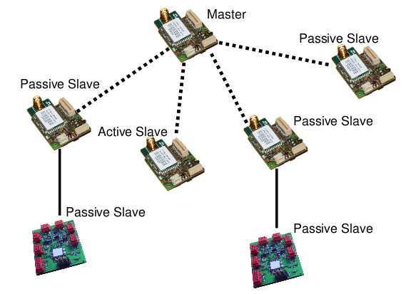
Figure 4: Experimental setup with six nodes building different kinds of slaves.

All nodes—the four iSense nodes and the two Atmels—were connected via wires to the interrupt lines of another microcontroller that measured the exact points in time when the nodes fired their events. Since the microcontroller was able to measure in terms of microseconds, we were able to obtain correspondingly accurate measurements.

IV-C Results

We ran several tests on our experimental setup. In each run, the master synchronized the network spontaneously, and sent a start message with different time intervals. We then measured the points in time when the nodes executed their tasks.

Event though the algorithm would be able to deal with multiple synchronization tasks at once—that is, a slave that synchronizes to more than one master in parallel, or a slave that also acts as a master—our experiments were only ran with one synchronization task per experiment. The main reasons for this decision was a simplified and more accurate measurement process, and a saving in code space, which was especially important for the Atmels.

Fig. 5 shows the absolute errors relative to the execution of the task at the master—as the average over all six nodes, both iSense and Atmel ones. The start interval has been increased consecutively from 50ms to 800ms.

Figure 5: Absolute error in execution of events; start interval 50ms to 800ms.

It can be seen that the average error is at approximately 1ms, regardless of the selected start interval. However, the greater the start interval becomes, the more outliers occur, and thus the maximal error increases to more than 5ms when selecting a starting time of 800ms. The maximal deviation in mainly caused by the very inaccurate Atmel ATmegas. This difference in accuracy between the iSense nodes and Atmels is shown in detail in Table III, which shows the error rates of all nodes in our network when the starting interval is set to 500ms.

TABLE III: Absolute Errors in ms on nodes with a start time of 500ms

Node	Min Err	Max Err	Avg Err	Stddev
Active Slave	0.004	1.455	0.640	0.389
Passive Slave 1	0.007	1.499	0.678	0.392
Passive Slave 2	0.006	1.463	0.734	0.375
Passive Slave 3	0.006	1.453	0.707	0.389
Atmel at PS 1	0.573	2.458	1.476	0.352
Atmel at PS 2	1.011	3.518	2.480	0.445

All four iSense nodes show very similar results. The minimal error is at only a few microseconds, whereas the maximal one is at most 1.5ms. In average, the deviation from the master is at around 700$\mu$s. In contrast to the iSense nodes, the Atmels show much worse results. The deviations are between 500$\mu$s and 3.5ms, with an average of 2ms. This is basically due to the inaccurate internal oscillator, which makes it impossible to calculate reliable clock drifts. However, for application areas where an event synchronization of only a few milliseconds is adequate, such as a synchronous playback of sound files or the concurrent sensing of a global event, the number of only five messages that are sent over the radio outperforms the inaccuracy.

Next, we also measured the propagation time of messages, both between the master and the active slave, and an iSense node connected to an Atmel via SPI. The result is shown in Fig. 6.

Figure 6: Propagation times over time.

The propagation time of the radio message varied between 2ms and 2.5ms, whereas the SPI communication was as expected constantly at 10us. The variance in wireless propagation time was mainly based on the need for an application-layer implementation.

V Conclusion

We presented an algorithm for the synchronous execution of tasks in sensor networks. In contrast to other well-known time synchronization algorithms, we do not provide a global time basis on the nodes. Instead, each node in the network is able to act spontaneously as a master, and let the remaining nodes execute a task at a certain point in the near future. The algorithm works in both hierarchical and heterogeneous systems. The former can be used to synchronize the network via multiple hops—if not all nodes are within communication range of the master. The latter means that we dealt with different kinds of hardware platforms and communication channels. Our experimental setup consisted of both limited platforms with very coarse clocks and nearly no code space, and ordinary sensor nodes with IEEE 802.15.4 compliant radios. The nodes used also both wireless and wired communication.

Sándor P. Fekete received his Diploma in Mathematics from the University of Cologne, Germany (1989), and his Doctoral Degree in Combinatorics and Optimization from the University of Waterloo Science, Canada (1992). After being a postdoc at SUNY Stony Brook (USA), he joined the Center for Parallel Computing in Germany in 1993 as an Assistant Professor, receiving his Habilitation in 1998. He was an Associate Professor at the TU Berlin in 1999-2001, and joined the Department of Optimization of the Braunschweig University of Technology in 2001.

In 2007 he became chair for Algorithmics in the Department of Computer Science. His research interests lie in both theoretical and practical aspects of algorithms, with a large variety of interdisciplinary collaborations. One of his main interests have been distributed algorithms, in particular in the context of large sensor networks.

Alexander Kröller received his Diploma in Mathematics from TU Berlin, Germany (2003), and his Doctoral Degree in Mathematics from Braunschweig University of Technology, Germany (2007).

He is currently an Academic Councilor at Braunschweig University of Technology, Germany. He was a postdoc at SUNY Stony Brook, USA (2008). He specializes in wireless sensor networks with a focus on distributed algorithms.

Tobias Baumgartner received his Diploma in Computer Science at Braunschweig University of Technology, Germany (2006).

He is currently a PhD student in the Algorithms Group of Prof. Fekete at Braunschweig University of Technology, Germany. In 2007, he worked as a Software Developer in the field of wireless sensor networks for ScatterWeb GmbH, Berlin, Germany. His main research interests are distributed algorithms for wireless sensor networks, and programming paradigms for tiny embedded systems—with a particular focus on sensor nodes.

Winfried Hellmann is a Bachelor student of Computer Science at Braunschweig University of Technology, Germany. His research interests lie in distributed algorithms for wireless sensor networks, and firmware development for embedded systems.

References

- [1] B. Sundararaman, U. Buy, and A. D. Kshemkalyani, “Clock synchronization for wireless sensor networks: a survey,” Ad Hoc Networks, 2005.
- [2] Y. R. Faizulkhakov, “Time synchronization methods for wireless sensor networks: A survey,” Program. Comput. Softw., vol. 33, no. 4, pp. 214–226, 2007.
- [3] K. Römer, “Time synchronization and localization in sensor networks,” Ph.D. dissertation, ETH Zürich, 2005, diss. ETH No. 16106.
- [4] J. Elson, L. Girod, and D. Estrin, “Fine-grained network time synchronization using reference broadcasts,” ACM SIGOPS Operating Systems Review, vol. 36, pp. 147–163, 2002.
- [5] S. Ganeriwal, R. Kumar, and M. B. Srivastava, “Timing-sync protocol for sensor networks,” in Proceedings of the 1st international conference on Embedded networked sensor systems, 2003, pp. 138–149.
- [6] S. Yoon, C. Veerarittiphan, and M. L. Sichitiu, “Tiny-sync: Tight time synchronization for wireless sensor networks,” ACM Transactions on Sensor Networks (TOSN), vol. 3, no. 2, p. 8, 2007.
- [7] H. Dai and R. Han, “Tsync: a lightweight bidirectional time synchronization service for wireless sensor networks,” ACM SIGMOBILE Mobile Computing and Communications Review, vol. 8, no. 1, pp. 125–139, 2004.
- [8] T. Baumgartner, S. Fekete, W. Hellmann, and A. Kröller, “Flash mob organization in heterogeneous wireless sensor networks,” in NTMS’09: Proceedings of the 3rd international conference on New technologies, mobility and security. Piscataway, NJ, USA: IEEE Press, 2009, pp. 487–490.
- [9] Atmel Corporation, “Atmega48/88/168,” 2009. [Online]. Available: http://www.atmel.com/dyn/resources/prod_ documents/doc2545.pdf
- [10] C. Buschmann and D. Pfisterer, “iSense: A modular hardware and software platform for wireless sensor networks,” 6. Fachgespräch Drahtlose Sensornetze der GI/ITG-Fachgruppe Kommunikation und Verteilte Systeme, Tech. Rep., 2007. [Online]. Available: http://ds.informatik.rwth-aachen.de/events/fgsn07
- [11] Jennic Ltd., “Product Brief JN513x, IEEE802.15.4 and ZigBee Wireless Microcontrollers,” 2007. [Online]. Available: http://www.jennic.com/files/product_briefs/JN513x_PB_ 160707_v1.2.pdf