Functional data analytic approach of modeling ECG T-wave shape to measure cardiovascular behavior

Abstract

The T-wave of an electrocardiogram (ECG) represents the ventricular repolarization that is critical in restoration of the heart muscle to a pre-contractile state prior to the next beat. Alterations in the T-wave reflect various cardiac conditions; and links between abnormal (prolonged) ventricular repolarization and malignant arrhythmias have been documented. Cardiac safety testing prior to approval of any new drug currently relies on two points of the ECG waveform: onset of the Q-wave and termination of the T-wave; and only a few beats are measured. Using functional data analysis, a statistical approach extracts a common shape for each subject (reference curve) from a sequence of beats, and then models the deviation of each curve in the sequence from that reference curve as a four-dimensional vector. The representation can be used to distinguish differences between beats or to model shape changes in a subject’s T-wave over time. This model provides physically interpretable parameters characterizing T-wave shape, and is robust to the determination of the endpoint of the T-wave. Thus, this dimension reduction methodology offers the strong potential for definition of more robust and more informative biomarkers of cardiac abnormalities than the QT (or QT corrected) interval in current use.

T1Supported in part by NISS and by Merck and Co.

and

1 Introduction

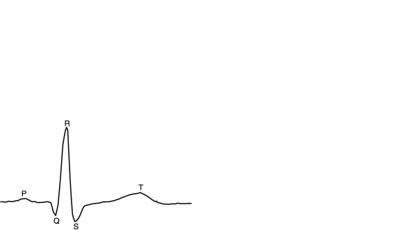
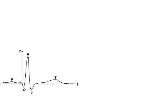
Electrocardiograms (ECGs) are widely used to screen and monitor the cardiac function of patients; and the behavior of the ECG wave form is a basis for diagnosis of specific abnormalities. Important wave forms of an ECG are marked by P, Q, R, S, T, as illustrated in Figure 1; these represent the changes in electrical potential as the heart contracts and relaxes. The T-wave represents the repolarization (or post-contractile phase) of the ventricles; and it is generally the most labile wave in the ECG. Abnormalities in the T-wave may be physiologic or may be externally induced, for example, by cardio-active drugs.

Figure 1: Features of a normal ECG.

The link between cardiac repolarization abnormalities and malignant arrhythmias, especially torsades de pointes (TdP), which may degenerate into ventricular fibrillation leading to sudden death, is well documented. Since some drugs, for example, haloperidol [FDA (2007)] and terfenadine [Morganroth, Brown and Critz (1993)], have been shown to cause repolarization abnormalities, testing for cardiac safety is required as a part of every new drug application to the FDA; and the FDA places very stringent constraints on the allowable prolongation of the repolarization process.

Figure 2: Two cardiologists’ marks of T-wave ends for 3 beats in a QT Dataset. The differences are 17 milliseconds (a), 15 milliseconds (b) and 104 milliseconds (c).

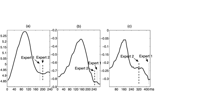
The current measure for cardiac safety that is used in drug development and drug approval is prolongation of the QT interval. The premise for using this measure is the evidence that the particular repolarization aberration, TdP, is either preceded by or characterized by a pro-arrhythmia defined in terms of delayed termination of the T-wave; more recently increased heterogeneity of T-waves has also been implicated [Couderc et al. (2009)]. The QT interval was first put forward in the 1920s and has been in continual use since, with little modification and with cardiologists personally marking the two critical points on the ECG: the initiation of the Q-wave and the termination of the T-wave. From a practical point of view, in a normal ECG of good quality, there is relatively little difficulty in the determination of the onset of the Q-wave even though an ECG has no actual “baseline.” However, measurement of the QT interval also relies on accurate and reproducible determination of the endpoint of the T-wave, which is a greater challenge, as can be seen from Figure 2. The differences between two cardiologists’ marks are 17 milliseconds in (a), 15 milliseconds in (b) and 104 milliseconds in (c). For QT analyses presented to the FDA, exceedance of 10 milliseconds for the maximal time difference between drug and control over all time points for a single patient calls into question the cardiac safety, requiring further discussion, at the least, before considering approval of the drug.

Thus, weaknesses of the current measurement method are four-fold: (1) QT as a cardiac safety indicator is predicated on detecting a heart-rhythm change associated (but not exclusively) with a particular cardiac arrhythmia. Slow trends, abrupt shifts in T-wave morphology, early precursors for T-wave changes and/or episodic events are not necessarily reflected. (2) The measurement ignores the information in the shape of the curve (the T-wave morphology), relying instead upon only two points of the complex curve. (3) Accuracy and the reproducibility of the measurement based on the endpoint of the T-wave depend on the sharpness of the T-wave form. (4) Current measurement practice calls for measuring and then averaging a sequence of a few (usually three) “highly similar” beats, most often from a 10-second record. (This 10-second sequence is often preselected by an algorithm that excludes difficult-to-read “outlier” beats and then captures a sequence for a near-constant heart rate, following 90 seconds of minuscule heart-rate variation. In this case, the cardiologist does not see the complete ECG, but only the selected beat sequence.)

In this paper a statistical model of the T-wave shape is constructed based on function data analysis (FDA), using all the data in an extended (minutes or longer) ECG record. This model has four interpretable parameters and performs well in describing both normal and arrhythmia ECGs available in public libraries. Because the parametrization of the model accounts for the morphology of the entire T-wave, it is particularly useful for describing changes in the repolarization process. It also has the significant advantage that it is robust to the determination of the onset or the end of the T-wave.

Effectively, this functional data analysis approach decomposes a sequence of T-waves for an individual subject into a reference curve (representing the common shape of the T-waves) and a four-dimensional representation of the deviation of each individual T-wave in the sequence. Inference about changes in cardiac function within the sequence can now be analyzed through the four-dimensional representation of individual T-waves. For multiple ECG sequences for the same subject, the reference curves for the individual sequences can be treated as data to again be analyzed by the appropriate construction of a (superpopulation) hyper-reference curve (representing the common shape of the reference curves) and four-dimensional representations of the “hyper-deviations” of each reference curve from the hyper-curve. In this fashion, the hyper-deviations can be used to analyze longer scale processes such as diurnal effects or shifts in baseline ECGs for long-term experiments.

Alternative methods to model the shape of ECG waves including the T-wave are principal component analysis (PCA) [Laguna et al. (1999)] and Gaussian models [Clifford (2006)]. Both methods fit the wave forms quite well and reduce the dimension of the data significantly. However, in terms of interpretation of model parameters, neither of them does well. The principal components and loadings in PCA do not provide physical interpretation of ECGs. The location and scale parameters in a Gaussian model may reveal some information about the shape of a T-wave, but they are not robust to small changes in T-waves such as those caused by noise. These features are shown in specific examples in Section 4.

The major difference between this FDA model and other models is that this model has a common reference curve for all the beats in the sequence and measures the deviation of each wave from the common curve. So it is most useful when one wants to compare the wave shape of a sequence of beats. All the other methods treat each wave separately, making it harder to compare model parameters across beats.

The ECGs examined in this research were all taken under normal clinical conditions and are digitized; they are in the public libraries through physionet (www.physiotnet.org). These ECGs include both normal subjects and subjects with various classes of arrhythmias and other cardiac function abnormalities; there are no data available (there or elsewhere) from actual QT studies since this data is proprietary and is held securely by the pharmaceutical companies.

Section 2 describes the preprocessing of a sample of the digitized ECG data before feeding it to the model, and lays out a general data structure to be studied. Section 3 describes the basic model, illustrates model robustness to the marking of T-wave boundaries, and shows the relation of model parameters to QT. In Section 4 statistical inference is shown on how to apply the model to T-wave analysis. Further issues and potential extension regarding the model and its applications are discussed on Section 5. Section 6 summarizes the conclusions from this research.

2 Description of data

2.1 One sample of ECG series

ECG data consist of a series of digitized waveforms, where the digitized value is the intensity of electrical potential (in millivolts) usually taken at a rate of 250 Hz (1 point per 4 milliseconds) or 1000 Hz (1 point per millisecond).

In order to make full use of the complete ECG record and to understand the natural variation of the T-wave over time, a natural representation is given by “stacking” aligned ECG segments of consecutive beats within a sample. To study the morphology of the T-wave, the stacked beats are left- and right-truncated uniformly, retaining the entire T-wave to form an $I\times J$ matrix $X=[x_{1},\ldots,x_{I}]^{T}$, where $x_{i}=[x_{it_{1}},\ldots,x_{it_{J}}]$ is the digitized value of T-wave during the interval of the $i$th beat and $I$ is the number of total beats in this record. Beats are aligned according to their QRS complexes since this complex is the most remarkable feature of ECG, and it allows the easiest and least variable alignment. While there are various methods for choosing the beginning and the end of T-waves, for example, the threshold method and the slope method [Panicker et al. (2006)], for the purpose of this study, the beginning and end points of the stacked T-waves are chosen to be identical for all the T-waves and to visually capture the shape of the T-waves. As will be shown later, the method described in this paper is robust to the choice of the beginning and end points. Having the beginning and end points equal for all beats is convenient for data analysis.

2.2 General data structure

A general data structure includes three levels: beat, sample and subject, one nested within another. In a typical study there are $P$ subjects, each subject has $Q_{p}$ samples, and each sample has $I_{pq}$ beats. Each beat has $J_{pq}$ time points within the T-wave interval. The data structure and notation is as follows:

• [$\bullet$]

• Subject $p$, $p=1,\ldots,P$.

• Sample $q$ (nested within subject $p$), $q=1,\ldots,Q_{p}$.

• Beat $i$ (nested within subject $p$ and sample $q$), $i=1,\ldots,I_{pq}$.

• Time point $t_{j}$, $j=1,\ldots,J_{pq}$.

• Digitized value $x_{it_{j}}$, $i=1,\ldots,I_{pq}$, $j=1,\ldots,J_{pq}$.

Note that all the data we use in this paper are digitized ECG data from PhysioNet (www.physionet.org), a public research resource website for physiologic signals. The sampling frequency is 250 Hz (250 points per second).

3 T-wave modeling using functional data analysis

3.1 A model based on modes of variation of functional data

Consider the data matrix $X$ for a sample ECG. Although $X$ involves only discrete values, it reflects smooth curves of T-waves that generate these values. As explained by Ramsay and Silverman [Ramsay and Silverman (1997)], this data matrix can be viewed as functional data since each row is a function of the time points at which they are measured, and these functions together form a family of functions. The goal here is to characterize each function in this family and to measure their variation.

One way to analyze functional data is to decompose variations along nonlinear directions from a common shape, denoted as the reference curve in this paper. Nonlinear decomposition of curves or multivariate data hasreceived much attention in the past twenty years. Hastie and Stuetzle[Hastie and Stuetzle (1989)] did pioneering work in defining and computing principal curves, which extend the linear PCA decomposition to nonlinear directions. Methods and applications based on principal curves are developed by Chalmond and Girard [Chalmond and Girard (1999)], Dong and McAvoy [Dong and McAvoy (1996)], etc. However, the nonlinear principal curves that are found to explain the most variation in data may not be interpretable, as is often true for principal components in linear PCA as well. Izem and Kingsolver [Izem and Kingsolver (2005)] built a 3-parameter shape invariant model that decomposes the variation in the data into predetermined and interpretable directions of interest. Their model describes the growth rate of families of caterpillars as a function of temperature:

$$z_{i}(t_{j})=w_{i}z\bigl{(}w_{i}(t_{j}-m_{i})\bigr{)}+h_{i}+\varepsilon_{i,j},$$ (1)

where $z_{i}(t_{j})$ is the growth rate of family $i$ at temperature $t_{j}$, $z$ is the common shape and $h_{i}$, $m_{i}$, $w_{i}$ represent the three modes of interest: vertical shift, horizontal location and norm-preserving slope change, respectively. A generalization of (1) is

$$z_{i}(t_{j})=R(\theta_{i},t_{j})+\varepsilon_{i,j},$$ (2)

where $z_{i}(t_{j})$ is a nonlinear function of time points $t_{j}$ and $\theta_{i}$ is the vector of parameters that represent fixed modes of variation.

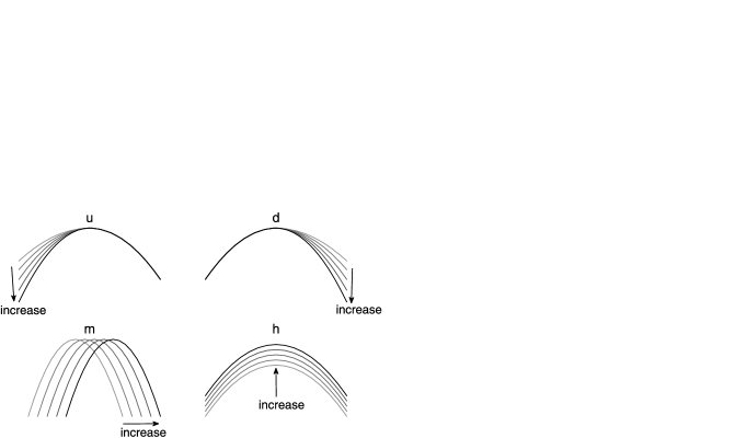
Motivated by their ideas, a model for T-waves is proposed as a combination of a reference curve and four fixed modes of variation that are of physiological interest: uphill slope, downhill slope, horizontal location and vertical shift. The reference curve represents the common shape of the T-wave; an element in the data matrix $X$ is modeled as

$$x_{it_{j}}=x_{i}(t_{j})=\cases{\sqrt{u_{i}d_{i}}K\bigl{(}u_{i}(t_{j}-m_{i})\bigr{)}+h_{i}+\varepsilon_{i}(t_{j}),&\quad$t_{j}\leq m_{i}$,\cr\sqrt{u_{i}d_{i}}K\bigl{(}d_{i}(t_{j}-m_{i})\bigr{)}+h_{i}+\varepsilon_{i}(t_{j}),&\quad$t_{j}>m_{i}$,}$$ (3)

where $i=1,\ldots,I$, $j=1,\ldots,J$, $K$ is the reference curve, the four parameters $u_{i}$, $d_{i}$, $m_{i}$, $h_{i}$ represent the uphill slope, downhill slope, horizontal location and vertical shift of the $i$th T wave, respectively, and $\varepsilon_{i}(t_{j})\sim N(0,\sigma^{2}_{i})$ is the error term. In light of (2),

$$R(\theta_{i},t_{j})=\cases{\sqrt{u_{i}d_{i}}K\bigl{(}u_{i}(t_{j}-m_{i})\bigr{)}+h_{i},&\quad$t_{j}\leq m_{i}$,\cr\sqrt{u_{i}d_{i}}K\bigl{(}d_{i}(t_{j}-m_{i})\bigr{)}+h_{i},&\quad$t_{j}>m_{i}$,}$$ (4)

where $\theta_{i}=(u_{i},d_{i},m_{i},h_{i})$. Figure 3 is a diagram of those four modes of variation.

Figure 3: Four modes of variation of T-waves: uphill slope change (u), downhill slope change (d), horizontal location (m) and vertical shift (h).

The model in (3) has two innovations over the 3-parameter shape invariant model in (1). First is the specification of a reference curve. A reference curve represents the common shape of all curves. It is the curve from which all the other curves are derived so that the estimated parameters of deformation can be compared and analyzed. A reference curve differs from the principal curve since the latter is mathematically defined to explain the most variation in the data. To measure the variation of curves within a sample, a natural choice of the reference curve is the Fréchet mean [Fréchet (1948)] of the curves in this sample. The Fréchet mean is a generalized mean on the nonlinear manifold, therefore, it represents the common shape of the curves. However, since the T-waves do not differ greatly in shape and location, nonparametric methods, such as spline interpolation of the pointwise average curve to obtain the reference curve, are effective and much less computationally intensive. (This is illustrated in Section 3.2.) The resulting curve is also much closer in shape to the data than a polynomial-based reference curve as used in Izem and Kingsolver (2005).

The concept of reference curve becomes crucial in a multiple sample analysis, such as a repeated measures design. A repeated measure design requires a single reference curve, usually a curve obtained from the baseline sample, so that the changes in the estimated parameters reflect the changes of the curves over time.

The second innovation is that this model is a piecewise function of the time points, since the uphill and downhill curves of the T-wave need to be modeled separately. This is due to the nature of the T-wave because the physiologic causes of deformation of the rise and of the decline of the T-wave can be quite distinct. This method also generalizes to a model with more piecewise functions that describe distinct shape changes over different time segments, allowing for more flexibility in modeling the overall shape.

Using the model in (3), each T-wave in a given set of T-waves can be rewritten as a transformation along fixed modes of variation from a reference curve. Further, such a transformation can be well approximated by four parameters representing these modes of variation. This simultaneously achieves significant dimension reduction of the data and a parametrization with physiological interpretations.

To estimate (3), minimize the sum of squares of the errors, that is, for each beat $i$,

$$\hat{\theta}_{i} = \operatorname{argmin}\limits_{\theta_{i}}\sum_{j}\bigl{(}x_{i}(t_{j})-R(\theta_{i},t_{j})\bigr{)}^{2},$$

where $R(\theta_{i},t_{j})$ is as in (4). Standard nonlinear optimization is used to estimate the parameters.

For computational accuracy and efficiency, the reference curves are centered at the origin both to facilitate the comparison of the parameter estimates curve to curve and also to minimize interpolation error. Since the support sets of the reference curve, K, and of X, the set of observed T-waves, can differ due to changes in the slope parameters, the support set for K must be extended beyond the support set of X to allow for interpolation at the endpoints. This causes interpolation error; centering the reference curve minimizes the change in the support set and hence reduces this error.

The multiplication factor $\sqrt{u_{i}d_{i}}$ in (3) also helps reduce the change in the support set for the same slope change, and hence reduces the interpolation error. Note that when $u_{i}=d_{i}$, this factor reduces to $u_{i}$, which can be regarded as a norm-preserving factor.

It is important to keep in mind that the interpretation of the four parameters is that they represent the vertical shift, horizontal location and slope changes of the WHOLE curve, not just any single point or small part of the curve. They give equal weight to all the points on the curve, and thus represent the curve better than measures that are taken from a few points on the curve, such as QT interval.

3.2 An illustration

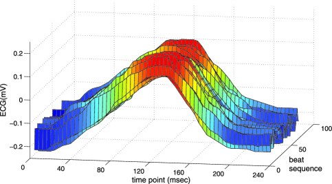
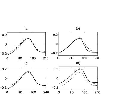
A simple example illustrates how the model works. A one-minute ECG record from the QT Database (Sel16265) with 66 beats is shown in Figure 4. The surface plot of the T-waves of this sample shows the T-waves “stacked” in sequence one behind the other. The color scale, used to accentuate the “surface geography” of the 3D plot, goes from cooler (blues) to warmer (reds) colors over the range from low to high. Beats are “stacked” in sequence one behind the other. In order to distinguish both the sequence and the color progression within each single T-wave, the color has been extended downward as vertical bars of the curve color. Visually, the common general character of these T-waves is easily described, as is the variation among them. We apply the model and fit 66 curves based on the reference curve that is obtained from the average of these 66 curves. Figure 5 shows the plots of the T-waves of 4 beats. The dashed lines are the reference curve that is identical for all beats. The dotted lines are the original T-waves and the solid lines are the fitted curves. Note that the vertical, horizontal and slope changes are captured very well by the fitted curves.

Figure 4: Surface plot of a sequence of T-waves of a sample ECG (the first-minute record of Sel16265).

3.3 Model robustness to marking of T-wave boundaries

Accurate determination of the end of the T-wave is widely acknowledged to be difficult. Therefore, a model that is based on T-wave morphology rather than T-wave boundaries and that is robust to marking those boundaries has great potential value. Figure 6 shows a T-wave with boundaries $[a,b]$ marked using standard software. Let

$$[a^{\prime},b^{\prime}]=[a+s,b-s],$$

Figure 5: Original T-waves (dotted lines), reference curve (dashed lines) and fitted curves (solid lines) for 4 beats of an ECG from the QT data base (Sel16265).

Figure 6: Diagram of change in T-wave boundaries as a function of $s$; $[a,b]$ is the T wave interval by the standard software. $s=-12,-4,+4,+12$ msec (for ECG at 250 Hz).

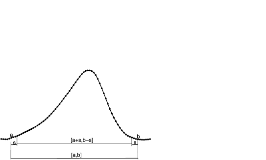
$s=-12,-4,4,12$ msec. As $s$ takes increasing values from $-$12 msec to $+$12 msec, the interval changes from the longest one [$a-12$ msec, $b+12$ msec] to the shortest [$a+12$ msec, $b-12$ msec], and the model parameters also change. Complete minute records of nine normal subjects are used for illustration. The robustness of the four parameter estimates is shown in Table 1. $\hat{u}_{[a,b]}$ is the estimate of $u$ at interval $[a,b]$, $\Delta\hat{u}$ is the difference between $\hat{u}$ at interval $[a+s,b-s]$ and $\hat{u}_{[a,b]}$, that is, $\Delta\hat{u}=\hat{u}_{[a+s,b-s]}-\hat{u}_{[a,b]}$. The same definitions apply to $d$, $m$ and $h$. Indicated in the first column, each measure, median or standard deviation, is adjusted by its scaling factor, to be comparable across parameters. Notice that both the medians and the standard deviations are small and are roughly of the same scale for all the parameters. For parameter $m$, the absolute change in the unit of milliseconds is also shown.

Table 1: Robustness of $(\hat{u},\hat{d},\hat{m},\hat{h})$ based on complete minute records for 9 normal subjects

Interval:	Longest				Shortest
	$\bolds{[a-12,b+12]}$	$\bolds{[a-4,b+4]}$	$\bolds{[a,b]}$	$\bolds{[a+4,b-4]}$	$\bolds{[a+12,b-12]}$
median$(\Delta\hat{u})/\hat{u}_{[a,b]}$	$-$0.0048.msec	$-$0.0024.msec	0	$-$0.0004.msec	$-$0.0010.msec
stdev$(\Delta\hat{u})/\hat{u}_{[a,b]}$	$-$0.0243.msec	$-$0.0096.msec	0	$-$0.0065.msec	$-$0.0107.msec
median$(\Delta\hat{d})/\hat{d}_{[a,b]}$	$-$0.0000.msec	$-$0.0009.msec	0	$-$0.0006.msec	$-$0.0002.msec
stdev$(\Delta\hat{d})/\hat{d}_{[a,b]}$	$-$0.0204.msec	$-$0.0079.msec	0	$-$0.0055.msec	$-$0.0119.msec
median$(\Delta\hat{h})/\hat{h}_{[a,b]}$	$-$0.0019.msec	$-$0.0023.msec	0	$-$0.0011.msec	$-$0.0012.msec
stdev$(\Delta\hat{h})/\hat{h}_{[a,b]}$	$-$0.0059.msec	$-$0.0063.msec	0	$-$0.0055.msec	$-$0.0064.msec
median$(\Delta\hat{m})/\hat{m}_{[a,b]}$	$-$0.0005.msec	$-$0.0000.msec	0	$-$0.0000.msec	$-$0.0001.msec
stdev$(\Delta\hat{m})/\hat{m}_{[a,b]}$	$-$0.0058.msec	$-$0.0014.msec	0	$-$0.0012.msec	$-$0.0020.msec
median$(\Delta\hat{m})$	$-$0.0131 msec	$-$0.0544 msec	0	$-$0.0395 msec	$-$0.1684 msec
stdev$(\Delta\hat{m})$	$-$0.3723 msec	$-$0.1825 msec	0	$-$0.2290 msec	$-$0.5124 msec

A plot provided courtesy of an anonymous referee shows two T-waves, one following the placebo, the other following administration of a positive control (amoxicillin). At hour 4, the percentage difference between uphill slopes for placebo and amoxicillin ($u_{p}$ and $u_{a}$, respectively) is $(u_{p}-u_{a})/u_{p}$, approximately 0.111. The downhill slope percentage difference $((d_{p}-d_{a})/d_{p})$ is roughly 0.156, the vertical percentage difference is roughly 0.111, and the horizontal percentage difference is roughly 0.083. Note that these differences substantially exceed the magnitude of change in the parameter estimates under different settings of the T-wave boundaries, as shown in Table 1. Thus, the analysis of T-wave morphology is sufficiently sensitive to detect these drug induced changes. The median and the standard deviation of $\Delta\hat{m}$, measured in milliseconds, also show that alteration of the T-wave boundaries do not present difficulties in the horizontal location estimate, given that the minimum critical change in the QT (cut-off value) is orders of magnitude higher, usually 10 milliseconds.

The 24 milliseconds range for $s$ (altering the interval length over a range of 48 milliseconds) was chosen to establish robustness for $(u_{i},d_{i},m_{i},h_{i})$ over a broad range for concern about QT prolongation based on FDA practice of seriously scrutinizing prolongations in excess of 10 milliseconds.

3.4 Relation of T-wave shape to QT

Effectively, the relationship between the four parameters that describe changes in the shape of the T-wave and changes in the QT interval is through translation and/or through flattening of the T-wave. As shown in Figure 7, measurement of QT can be depicted by placing one beat on a plane where the baseline matches the horizontal axis, $t$, and with the origin placed at the initiation of the Q-wave. The QT interval then ends approximately where the T-wave intersects the horizontal axis on its right. To see the relationship between the four parameters and QT, first consider their relationship to be a (less complicated) quadratic form:

$$K(t)=a(t-b)^{2}+c,\qquad a<0,c>0;$$ (5)

QT can be calculated explicitly:

$$QT=b+\sqrt{-\frac{c}{a}}.$$ (6)

Let $\tilde{K}(t)$ be the quadratic function written in the form of the model in (3),

$$\tilde{K}(t) = \cases{\sqrt{u_{i}d_{i}}\bigl{[}a\bigl{(}u_{i}(t-m_{i})-b\bigr{)}^{2}+c\bigr{]}+h_{i},&\quad$t\leq m_{i}$,\cr\sqrt{u_{i}d_{i}}\bigl{[}a\bigl{(}d_{i}(t-m_{i})-b\bigr{)}^{2}+c\bigr{]}+h_{i},&\quad$t>m_{i}$.}$$

Thus,

$$\tilde{QT}=\cases{m_{i}+\dfrac{b}{u_{i}}+\dfrac{1}{u_{i}}\sqrt{-\dfrac{c}{a}-\dfrac{h}{a\sqrt{u_{i}d_{i}}}},&\quad$t\leq m_{i}$,\cr m_{i}+\dfrac{b}{d_{i}}+\dfrac{1}{d_{i}}\sqrt{-\dfrac{c}{a}-\dfrac{h}{a\sqrt{u_{i}d_{i}}}},&\quad$t>m_{i}$.}$$ (7)

Figure 7: To quantify the relationship between QT and four parameters, the ECG of one beat is placed on a plane where the baseline matches the horizontal axis $t$, and the start of Q is placed at the origin. For convenience, QT is measured from the origin to the point where the T-wave intersects the horizontal axis on its right.

From (7) the dependence of QT on $m$ is seen to be direct and positive, while dependence on $u$ and on $d$ is inverse. The relationship of $(h)^{1/2}$ to QT is direct, but also involves both $u$ and $d$. Therefore, when, as can occur in practice, the data show $\hat{h}$ to be correlated with $\hat{u}$ and/or $\hat{d}$, the observed QT may or may not exhibit a positive simple correlation of QT with $\hat{h}$.

Figure 8: Four parameter estimates versus QT (Sel103) showing correlations with $\hat{m}$ (positive) and $\hat{u}$ (negative).

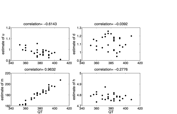
One example that serves as an illustration is a half-minute record (Sel103), an arrhythmia from the QT Dataset (with QT calculated using ECGpuwave software also available on www.physionet.org). Figure 8 shows the scatterplots of the parameter estimates and QT intervals. For this record, QT dependence on $\hat{m}$ is evidenced in their positive correlation ($r=0.9632$), indicating that the T-wave shifts to the right to increase QT. The negative correlation between $\hat{u}$ and QT means that as the uphill curve flattens, QT gets longer. This confirms expert qualitative statements about T-wave changes.

4 Statistical inference

The principal objectives for a functional data analysis approach to analyze sequential T-waves are as follows: (1) to use information for the complete form of a T-wave, (2) to capture full information for an extended series of beats, and (3) to define a low-dimensional parametrization model to use in drawing statistical inferences.

Consider the problem arising in analysis of an arrhythmia: classification of beats according to the shape of their T-waves. Clustering similar beats in ECGs is the first step in identifying patterns of beats that characterize specific cardiac function abnormalities. For example, if a cluster of similar beats is defined in terms of the parameter $h$ (and not dependent upon $u$, $d$ or $m$), then the types of beats differ by the T-wave heights, that is, by the signal intensity not by its pattern. In contrast, multivariate-defined clusters differ according to the signal patterns and possibly the signal intensity.

Figure 9: A sample ECG for patient Sel104.

Figure 10: Normal (circle) and abnormal (star) beats, plotted vs (a) RR and (b) QT.

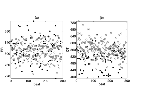
Figure 9 shows a sequence of the ECG tracing of an arrhythmia subject Sel104 from the QT Dataset (a four-minute record with 292 beats). Visually there are two major types of beats: one type with normal T-waves and the other type with “S” shape T-waves. Figure 10 shows that neither the beat length (RR: interval from preceding R peak to succeeding one) nor QT successfully discriminates between these two types of beats. (Here the QT intervals are obtained by applying ECGpuwave software followed by confirmation or correction by expert review.)

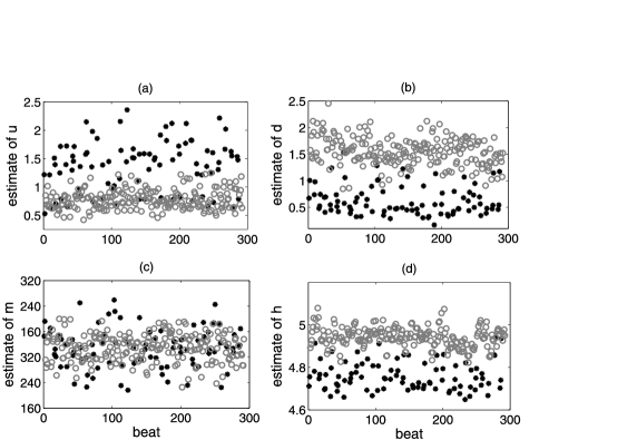
Figure 11 shows the plots of $\hat{u}$, $\hat{d}$, $\hat{m}$ and $\hat{h}$ in (a), (b), (c) and (d), respectively. Observe that both $\hat{d}$ and $\hat{h}$ do well in separating these two groups. In fact, using K-means clustering for $\hat{d}$, one can get two clusters that match (95.35% of beats) with the two groups. $\hat{u}$ also does a fairly good job, but $\hat{m}$ does not distinguish the two groups.

Figure 11: Normal (circle) and abnormal (star) beats for a 4-minute record (292 beats) of Sel104, plotted as time series of (a) $\hat{u}$ (b) $\hat{d}$ (c) $\hat{m}$ and (d) $\hat{h}$.

An alternative method for modeling T-wave shape uses two Gaussians. Approximation of a single T-wave as a mixture of two Gaussians can be quite precise [Clifford (2006)]; this can be combined with a suitable algorithm to define the end of T-wave in terms of a specified tail probability. However, this exercise is (independent) curve fitting to individual beats, hence is not amenable to further statistical inference.

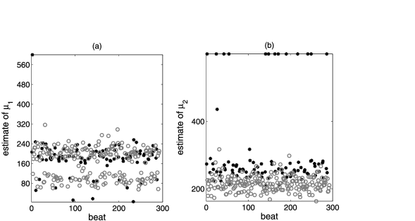
Figure 12 plots the means $(\mu_{1},\mu_{2})$ of the left and right Gaussians fitted as a mixture. The left Gaussian which dominates the onset of the T-wave does not discriminate between beat types. The right Gaussian which dominates extreme tail behavior is only partially successful, with an overall misclassification rate of $26.73\%$. (By comparison, the overall misclassification rate using the four-parameter model is $4.65\%$.) However, inferences about the typical shape of each type of T-wave remains difficult. This is due in part to the number of estimated parameters (6 for each beat) and in part to the instability of the parametrization. In fact, parametrization of the Gaussian model is not robust to small changes in T-wave shape, such as those caused by noise. As an illustration, Figure 13 shows 2 T-waves in record Sel104. The very slight difference in the last part of the two T-waves induces two very different parametrizations. For the first T-wave in (a), the two Gaussian functions are almost identical. The parametrization $(\lambda_{i},\sigma_{i}^{2},\mu_{i})$, where $\lambda_{i}$ is the unnormalized mixing coefficient for the $i$th Gaussian, is (4.5102, 19.5607, 44.4245) for the first Gaussian and (4.5102, 19.5588, 44.4265) for the second Gaussian; and the two Gaussian curves are seen to overlap in Figure 13(a), while for the second T-wave in (b) the two sets of parameters are quite different: (3.3558, 11.0680, 27.8644) and (6.9715, 18.7290, 55.7295), and the Gaussians separate as shown in Figure 13(b). Thus, the parameters for the Gaussian model cannot accurately reflect the degree of difference among curves, and hence do not make a good biomarker for analysis of T-wave shape or statistical inference about beat problems.

Figure 12: Normal (circle) and abnormal (star) beats, plotted vs (a) the first location parameter $\mu_{1}$ of a Gaussian model and (b) the second location parameter $\mu_{2}$ of a Gaussian model.

Figure 13: Two similar T-waves (solid lines) in record Sel104, with two Gaussian functions (dashed lines and dotted lines) fitted to each by the Gaussian model.

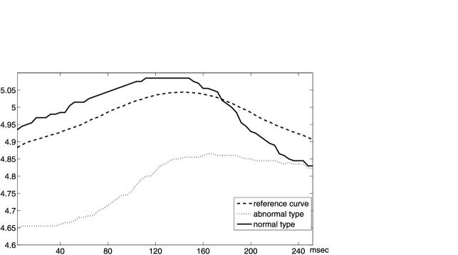
There are other methods that work well in classifying curves, such as wavelet-based methods [Wang, Ray and Mallick (2007)], or even PCA; but neither wavelet coefficients nor principal components of the curves help to understand the physiological change in the shape of the T-wave. From the sequences of four parameter estimates one can obtain more information about the different shape of the T-wave for different groups. For example, by inspecting Figure 11, one observes that, among the two groups, one group has higher $\hat{u}$ (greater than 1), lower $\hat{d}$ (less than 1), lower $\hat{h}$ and similar $\hat{m}$ as the other. Note that for $\hat{u}$ and $\hat{d}$, 1 is a cut-off value because when $\hat{u}>1$, the uphill curve is steeper than the reference curve, elsewhere it is flatter. The same applies to $\hat{d}$. So it can be imagined that one group of beats has steeper uphill curve, flatter downhill curve and lower height than the reference curve. The other group behaves conversely. The horizontal positions do not distinguish the two. These descriptions match the true curves as shown in Figure 14.

Figure 14: The reference curve and typical curves of the two types of T-waves in Sel104.

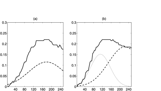
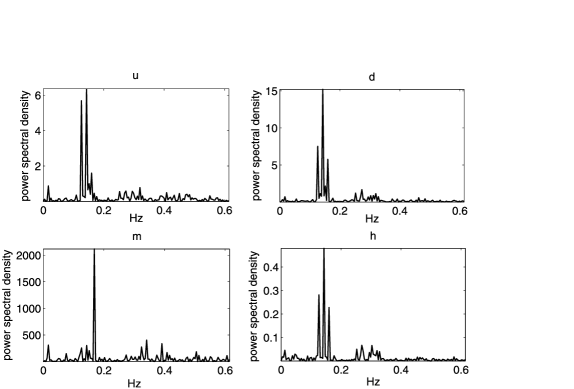
Furthermore, one can obtain information about T-wave shape change by studying the parameter estimates over beats as four time series. To study the frequency components of these time series, one can obtain the power spectral density, shown in Figure 15. Note that $\hat{u}$, $\hat{d}$ and $\hat{h}$ all have peaks at 0.1265 Hz, 0.1429 Hz and 0.1592 Hz, corresponding to periods 7.9 sec (9.6 beats), 7 sec (8.51 beats) and 6.28 sec (7.64 beats). These are roughly the frequencies of the abnormal beats that can be observed from the ECG chart. $\hat{m}$ has a peak at 0.1674 Hz, corresponding to 5.97 sec (7.2 beats). Since $\hat{m}$ is most correlated with RR among the four parameters (see Figure 16), and regular changes in RR are usually related to breathing, a reasonable guess is that this frequency reflects the breathing pattern of this subject. Many other properties in the time domain and frequency domain can be studied as well.

Figure 15: The power spectral density of $\hat{u}$, $\hat{d}$, $\hat{m}$ and $\hat{h}$.

In order to make comparisons between time segments or between experimental conditions, the QT measure needs to be adjusted by the RR (the inverse of the heart rate) because of the relationship long-recognized between the two. Although the literature on choices of adjustment function is extensive, no consensus has been reached on the optimal “correction” or adjustment function. This may be at least partially attributable to the disparity in changes in the QT and in the TQ intervals with change in RR, especially in normal subjects. Adjustment methods for the four-parameter model will depend on the direct relationship of the T-wave shape and RR; and this relationship may differ between normal subjects or among subjects with different known arrhythmias. Also, the dependence between RR and the onset of T-wave shape alteration may exhibit a lag of several beats.

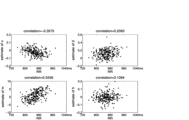
The first example, shown in Figure 16, is a four-minute record of an arrhythmia subject Sel103 from the QT Dataset. Here $\hat{u}$ and RR are modestly negatively correlated, which means that as uphill curve gets flatter, RR gets longer. The positive correlation of $\hat{m}$ and RR means that the RR prolongation is generally related to a T-wave shift to the right. Relationships of $\hat{d}$ and $\hat{h}$ with RR are not apparent in this record. This data set benefits from a multivariate clustering approach since several individual relationships between model parameter estimates and RR are accompanied by interdependencies among the parameters. Further analysis shows that $\hat{u}$ and $\hat{d}$ are negatively correlated in this case, that is, the uphill curve and downhill curve change their slopes in such a way as to keep the angle between them relatively stable.

Figure 16: Correlations of four parameter estimates with RR (Sel103).

Different arrhythmias exhibit different patterns and may arise from different causes; the four-parameter model enables inferences about these patterns. A second example illustrates a different phenomenon. In this arrhythmia, the sequence of beats can be shown to have an approximate periodicity. By representing this record as a series of four-dimensional vectors $(\hat{u},\hat{d},\hat{m},\hat{h})^{\prime}$, the lag of principal time-dependency can be established. Table 2 shows the correlation of each parameter at time $t$ with RR at time $t$, $t-1$, $t-2$ and $t-3$ for the 2nd minute of the record of Sel123 from the QT Dataset. Note that all the parameters are most strongly correlated with RR at $(t-2)$, indicating a two-beat lag between RR and the altered T-wave. Thus, a longer beat is followed by alteration in the T-wave form (shallower). Physiologically this may have explanation in terms of energy expenditure and the adequacy of the “rest” between the end of the T-wave and the onset of the subsequent P-wave. The last row indicates that QT does not capture such a phenomenon.

5 Discussion

Besides the applications mentioned in Section 4, there are others such as outlier beat detection and discrimination between normal subjects and arrhythmia subjects. One can detect outlier beats by treating the four parameters’ values as four-dimensional vector data and applying standard outlier detection methods for multivariate data. Distinguishing arrhythmias from normal heart rhythms can be done based on the patterns of variation in this four-dimensional characterization. Work is ongoing to develop specific methodology to encompass beat classification and analysis of the temporal process.

Methods for analyzing data with a general data structure described in Section 2.2 depend on the purpose of the study. For the measurement of T-wave variation within each sample, for example, detection of outlier beats within a record, the reference curve can be computed as the pointwise average curve for the record, and the analysis is based on the parameter estimates for the curves in that record. For multiple records of the same subject, a “super-reference curve” can be computed, by analogy to MANOVA methodology, the parameter estimates using the within-record reference curve and those computed using the super-reference curve can be analyzed. (This approach inherits the same problems of unequal variances and unequal sample sizes that are present in MANOVA analyses with essentially the same solutions.)

=200pt RR $\bolds{t}$ $\bolds{t-1}$ $\bolds{t-2}$ $\bolds{t-3}$ $\hat{u}$ $-$0.3216 $-$0.4003 $\bolds{-}$0.7554 $-$0.3152 $\hat{d}$ $-$0.4580 $-$0.6309 $\bolds{-}$0.7428 $-$0.3957 $\hat{m}$ $-$0.3009 $-$0.3419 $-$0.4596 $-$0.1900 $\hat{h}$ $-$0.2410 $-$0.1825 $\bolds{-}$0.3977 $-$0.0605 QT $-$0.0478 $-$0.1953 $-$0.1646 $-$0.0455

Table 2: Correlation between the estimated model parameters and current and previous $RR$s

For complex experiment designs with ECGs taken repeatedly over time and/or under varying conditions, the actual time courses of T-wave changes as well as variation may be the primary focus. (For example, in a study of a new drug, ECGs may be conducted for each subject at a dozen time points each day beginning with a baseline—none, placebo, positive control substance, drug, etc.) In such a case the reference curves for individual records within each set form a data set of curves to be studied. Once again, applying a functional analysis approach, a hyper-reference curve can be computed (from the record reference curves) and analyzed.

The functional data approach used here could also be extended to alternative choices of the reference curve. For example, robust methods could be applied to reduce the influence of outlier beats. In the case when there are clusters of beats varying by shape, such as in Figure 9, this approach may first be applied to cluster beats, as described in Section 4, then it is applied within each cluster to capture the individual differences within the cluster.

Extension of the method proposed here to multi-lead ECG data is direct. Standard 12- or 16-lead ECGs provide spatial information about the heart as well as redundancies and “check information.” Current work combines dimension reduction methods with this functional data modeling approach to more fully incorporate the information from multiple leads without decreasing the signal-to-noise ratio. In addition, since specific leads measure the electrical potential across different parts of the heart, the extension to a higher dimensional model should lead to a more general methodology and increase sensitivity to other aberrant cardiac behaviors.

6 Conclusion

In this paper functional data analysis is used to construct a statistical model of ECG T-waves. This model makes the physiologically reasonable assumption that there is a common primary shape (within subject) for the T-waves and it uses four interpretable parameters to describe the individual deviation of each beat from the common T-wave shape. The model accounts for the entire T-wave morphology, making the estimation robust to the marking of T-wave boundaries. Applications such as classification of beats were illustrated for this model. Application of this model to measuring drug-induced change in T-wave is intended, pending availability of control ECGs from actual QT studies.

Note: Programs in matlab to implement the method are available from the authors. Please send requests by email to label=e3]yingchun_z@yahoo.come3.

References

- FDA (2007) http://www.fda.gov/Drugs/DrugSafety/PostmarketDrugSafetyInformationforPatients andProviders/DrugSafetyInformationforHeathcareProfessionals/ucm085203.htm.
- Chalmond and Girard (1999) Chalmond, B. and Girard, S. (1999). Nonlinear modeling of scattered multivariate data and its application to shape change. IEEE Transactions on Pattern Analysis and Machine Intelligence 21 422–432.
- Clifford (2006) Clifford, G. D. (2006). A novel framework for signal representation and source separation: Applications to filtering and segmentation of biosignals. Journal of Biological Systems 14 169–183.
- Couderc et al. (2009) Couderc, J. P., Kaab, S., Hinterseer, M., McNitt, S., Xia, X., Fossa, A., Beckmann, B. M., Polonsky, S. and Zareba, W. (2009). Baseline values and sotalol-induced changes of ventricular repolarization duration, heterogeneity, and instability in patients with a history of drug-induced torsades de pointes. Journal of Clinical Pharmacology 49 6–16.
- Dong and McAvoy (1996) Dong, D. and McAvoy, T. (1996). Nonlinear principal component analysis-based on principal curves and neural networks. Computers and Chemical Engineering 20 65–78.
- Fréchet (1948) Fréchet, M. (1948). Les éléments aléatoires de nature quelconque dans un espace distancié. Ann. Inst. H. Poincaré 10 215–310. \MR0027464
- Hastie and Stuetzle (1989) Hastie, T. and Stuetzle, W. (1989). Principal curves. J. Amer. Statist. Assoc. 84 502–516. \MR1010339
- Izem and Kingsolver (2005) Izem, R. and Kingsolver, J. (2005). Variation in continuous reaction norms: Quantifying directions of biological interest. The American Naturalist 166 277–289.
- Laguna et al. (1999) Laguna, P., Moody, G. B., Garcia, J., Goldberger, A. L. and Mark, R. G. (1999). Analysis of the st-t complex of the electrocardiogram using the karhunen-loeve transform: Adaptive monitoring and alternans detection. Medical and Biological Engineering and Computing 37 175–189.
- Morganroth, Brown and Critz (1993) Morganroth, J., Brown, A. M. and Critz, S. (1993). Variability of the QTc interval: Impact on defining drug effect and low-frequency cardiac event. The American Journal of Cardiology 72 B26–B31.
- Panicker et al. (2006) Panicker, G. K., Karnad, D. R., Joshi, R., Kothari, S., Narula, D. and Lokhandwala, Y. (2006). Comparison of QT measurement by tangent method and threshold method. Indian Heart Journal 58 487–488.
- Ramsay and Silverman (1997) Ramsay, J. and Silverman, B. (1997). Functional Data Analysis. Springer, New York. \MR2168993
- Wang, Ray and Mallick (2007) Wang, X., Ray, S. and Mallick, B. K. (2007). Baysian curve classification using wavelets. J. Amer. Statist. Assoc. 102 962–973. \MR2354408