Integral field spectroscopy of H₂ and CO emission in IRAS 18276-1431: evidence for ongoing post-AGB mass loss

Abstract

We present K-band integral field spectroscopy of the bipolar post-AGB object IRAS 18276-1431 (OH 17.7-2.0) using SINFONI on the VLT. This allows us to image both the continuum and molecular features in this object from $1.95-2.45\mu$m with a spatial resolution down to 70 mas and a spectral resolution of $\sim 5000$. We detect a range of H₂ ro-vibrational emission lines which are consistent with shock excitation in regions of dense ($\sim 10^{7}$ cm^-3) gas with shock velocities in the range $25-30$ km s^-1. The distribution of H₂ emission in the bipolar lobes suggests that a fast wind is impinging on material in the cavity walls and tips. H₂ emission is also seen along a line of sight close to the obscured star as well as in the equatorial region to either side of the stellar position which has the appearance of a ring with radius 0.3 arcsec. This latter feature may be radially cospatial with the boundary between the AGB and post-AGB winds. The first overtone ¹²CO bandheads are observed longward of 2.29 $\mu$m with the ${\rm v}=2-0$ bandhead prominently in emission. The CO emission has the same spatial distribution as the K-band continuum and therefore originates from an unresolved central source close to the star. We interpret this as evidence for ongoing mass loss in this object. This conclusion is further supported by a rising K-band continuum indicating the presence of warm dust close to the star, possibly down to the condensation radius. The red-shifted scattered peak of the CO bandhead is used to estimate a dust velocity along the bipolar axis of 95 km s^-1 for the collimated wind. This places a lower limit of $\sim 125$ yr on the age of the bipolar cavities, meaning that the collimated fast wind turned on very soon after the cessation of AGB mass loss.

1 Introduction

Imaging surveys of young post-asymptotic giant branch (post-AGB) stars, not yet hot enough to ionize their envelopes, show that many are already associated with complex nebulosities. They exhibit a range of structural symmetries, such as bipolar, multipolar and point-symmetric (e.g. Siódmiak et al. 2008, Sahai et al. 2007, and references therein). These objects then evolve into ionized planetary nebulae (PNe) with similar morphologies which strongly suggests that (i) the shaping process operates and is largely completed during this earlier pre-PN phase and (ii) the onset of shaping may be linked with the appearance of a collimated fast wind early in the post-AGB phase, which then carves axisymmetric channels into the remnant AGB envelope (e.g. Sahai & Trauger 1998; Lee, Hsu & Sahai 2009).

The appearance of fast collimated winds at the end of the AGB is linked with the emergence of collisionally excited molecular transitions (e.g. Davis et al. 2005). In particular, the K-band ro-vibrational transitions of H₂ will be excited, and these provide an important tracer of shocked gas in pre-PNe. Imaging and spectroscopic surveys (e.g. Hrivnak, Kwok & Geballe 1994; García-Hernández et al. 2002; Davis et al. 2003, 2005; Kelly & Hrivnak 2005) show that, for spectral types later than B, the stellar UV flux is still not usually sufficient for radiative excitation to dominate and so the H₂ emission is produced in shocks. There appears to be a strong correlation between shock-excited H₂ and bipolarity, something that has also been noted for PNe (Kastner et al. 1996).

IRAS 18276-1431 (OH 17.7-2.0) is a fairly well studied post-AGB object and a review of its properties is given by Bains et al. (2003). These authors present interferometry and polarimetry of the OH maser lines, showing evidence for a molecular torus expanding slowly at 13 km s^-1, threaded by an ordered magnetic field. In the near-IR the object has a bipolar appearance and imaging polarimetry in the K-band shows that the lobes are seen in scattered light with the source remaining hidden (Gledhill 2005). High angular resolution imaging in the $K_{p}$-, $L_{p}$- and $M_{s}$-bands reveals the structural details of the lobes and halo, including searchlight beams and concentric multiple arcs (Sánchez Contreras et al. 2007; hereafter SC07). These authors also present CO interferometry observations and a spherically symmetric radiative transfer model of the spectral energy distribution (SED).

The near-IR continuum observations provide information on the distribution of dust and optical depth throughout the object; the bipolar structures nested within a more spherical halo suggest the recent development of axisymmetry linked to the onset of a collimated post-AGB wind. In this paper we concentrate on the molecular emission, its excitation and the interaction between any collimated outflow and the AGB envelope in IRAS 18276-1431 (hereafter IRAS 18276). We present integral field spectroscopy using the SINFONI instrument on VLT, which allows us to map the distribution of the various K-band molecular emission features over the object.

2 Observations and data reduction

Observations of IRAS 18276 were made on 2005 June 30 with the SINFONI integral field spectrometer on the 8.2-m UT4 telescope at the VLT observatory in Chile (Eisenhauer et al. 2003, Bonnet et al. 2004). The K-band grating was used covering a wavelength range of $1.95$ to $2.45~{}\mu$m with spectral resolution of $\sim 5000$. This equates to a spectral pixel (channel) width of $2.45\times 10^{-4}~{}\mu$m. The expected spectral resolution is 2 channels or $4.9\times 10^{-4}~{}\mu$m ($\approx 66$ km s^-1 at $2.2~{}\mu$m). Both Medium Resolution Mode (MRM) and High Resolution Mode (HRM) observations were made.

In MRM mode, the field of view is 3$\times$3 arcsec with $50\times 100$ mas spatial pixels. A total of 6 integrations were made, at two overlapping pointings, so that the total integration time on IRAS 18276 was $6\times 200$ sec = 20 min. Offset sky exposures were obtained along with the standard arc, flux and telluric calibrations. Flux and telluric calibration was performed using HIP 85920. The airmass range of these observations was $1.023-1.060$ with an ambient seeing of $\approx 0.8$ arcsec. AO-correction in MRM resulted in an average PSF of 150 mas FWHM (measured using the field star FS1 - see Fig. 1a).

HRM provides a field of view of $0.8\times 0.8$ arcsec with $12.5\times 25$ mas pixels. The HRM observations were obtained at high airmass at the end of the night as the object was setting. Telluric correction of these observations proved difficult and in the end we rejected all but 3 data sets, where the airmass was less than 1.9. A single pointing was used in these observations so that the total integration time on-source is $3\times 300$ sec = 14 min. HIP 18302 was used as the flux and telluric standard. Ambient seeing was again $\approx 0.8$ arcsec and AO correction resulted in a PSF width of $\approx 70$ mas FWHM estimated from the standard star.

The MRM and HRM data were reduced in a common manner using the ESO pipeline for SINFONI with further processing and data visualization using the STARLINK software collection.

3 Results

3.1 White light images

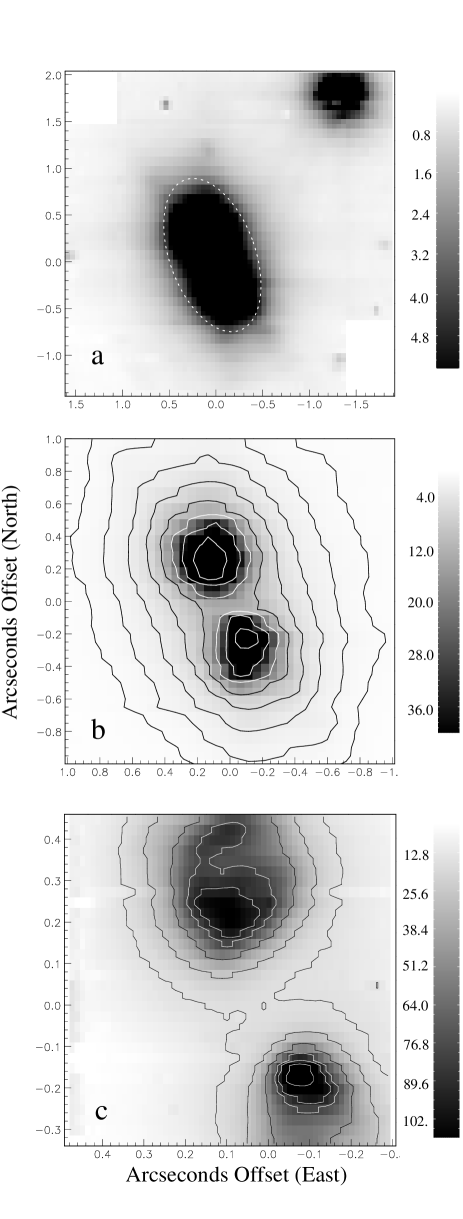
Figure 1: K-band ‘white light’ images of IRAS 18276. MRM images show the faint (a) and bright (b) emission. Contours in (b) are at 0.8, 1.5, 2.9, 5.5, 10.6, 20.1, 38.3, 72.9. The dotted ellipse shows the region over which the K-band spectrum (Fig. 2) is extracted. The star to the top right in (a) is the field star FS1 (see text). In (c) we show the HRM image. Contour levels in this image are at 15.4, 25.6, 47.4, 79.4, 94.7, 126.7. All greyscale and contours levels are in units of 10^-15 W m^-2 arcsec^-2.

The SINFONI spectral datacube can be collapsed along the wavelength axis to produce a ‘white light’ image. In Fig. 1 we show the MRM and HRM data summed over the range 1.95–2.45 $\mu$m, to form white light images of the object, dominated by the scattered continuum emission. The upper panel (Fig. 1a) displays the entire SINFONI field, comprising two telescope pointings, and shows the faint emission levels. The star to the upper right was identified as a field star, not physically associated with IRAS 18276, in J- and K-band polarimetric observations (Gledhill 2005) and is the star labelled ‘FS1’ by SC07. The four searchlight beams identified by SC07 are visible, extending through the faint halo.

In the central panel (Fig. 1b), the brighter continuum emission is shown, revealing two lobes either side of the central position, forming a bipolar nebula. Polarimetric observations show high degrees of linear polarization in the lobes ($\approx 50$ per cent in the K-band) confirming that the nebulosity is seen by scattered light (Gledhill 2005). The star is hidden by a circumstellar torus of dust and gas completely obscuring the direct view at these wavelengths. SC07 estimate a lower limit to the optical depth of the circumstellar obscuration at 2.12 $\mu$m of $\tau_{2.12}>12.3$. We define the origin of our coordinate system in these images as the centre of the obscuring lane along a line joining the brightness peaks of the two lobes.

The HRM image, shown in Fig. 1c, provides a field of view of $0.8\times 0.8$ arcsec and close to diffraction-limited imaging on the 8.2-m VLT. The origin of the coordinate system is located as before, at the centre of the obscuring lane midway between the two lobes. The structure in the HRM image closely resembles that seen in the sharpened K_p Keck telescope image of SC07, with the limb-brightened tip or ‘cap’ clearly visible in the northern lobe. The axis defined by the two continuum peaks lies at a position angle (PA) of 24°.

The K-band flux density is $88\pm 3$ mJy (the error mainly coming from the telluric correction), corresponding to $K=9.67\pm 0.04$ mag. This agrees reasonably with the flux density of 96 mJy quoted by SC07 for observations just 1 month after our own. There is also agreement within errors with the $K=9.5\pm 0.3$ measurement of July 2001 (Gledhill 2005).

3.2 Integrated spectrum

The spectrum of IRAS 18276, from 1.95–2.45 $\mu$m, after telluric correction and flux calibration, is shown in Fig. 2, and is integrated over the elliptical aperture shown in Fig. 1a. The continuum rises smoothly throughout the K-band and originates mainly from the bipolar lobes, where light from the hidden central source is scattered into our line of sight by dust grains. Superimposed on the continuum there are numerous emission features corresponding to the S- and Q-branch ro-vibrational transitions of H₂, which are labelled. We label the first four ¹²CO overtone bandheads, which are prominent in emission longward of 2.29 $\mu$m. We also detect the Na I doublet lines in emission around 2.2 $\mu$m. We do not detect Br$\gamma$. Other emission features in the spectrum result from incomplete correction for metal absorption lines in the telluric standard.

3.3 Continuum subtraction and line flux estimation

In order to get a good fit to the continuum in the vicinity of each emission line, the K-band spectral cube was sectioned, in the wavelength direction, into smaller ‘line cubes’, each containing a single emission line and surrounding continuum. A linear fit was then made to the continuum on either side of the line, extrapolating under the line. The MFITTREND application, part of the STARLINK software collection, was used to perform this fit along the wavelength direction for each spatial pixel in the line cube, producing a continuum cube. The continuum cube was then subtracted from the line cube to leave a continuum-subtracted spectral cube containing the emission line.

To estimate the flux in a line, aperture photometry using an elliptical aperture was performed for each spectral image (channel) in the cube containing flux above the background noise. The fluxes estimated for each H₂ line and for the ${\rm v}=2-0$ CO bandhead emission are given in Table 1 along with the rest and observed wavelengths of the lines. The H₂ line peaks are consistently offset to the red of the rest wavelength, with an average offset of $4\pm 1\times 10^{-4}$ $\mu$m (a wavelength channel is $2.45\times 10^{-4}$ $\mu$m) whereas the CO bandhead peak is offset to the red by $1.3\times 10^{-3}$ $\mu$m. The velocity structure of the emission is discussed further in Section 7.

Figure 2: The integrated spectrum of IRAS 18276 between 1.95 and 2.45 $\mu$m, showing the $1-0$ and $2-1$ H₂ ro-vibrational lines, CO first overtone bandheads and Na I lines. Other emission features result from residual metal absorption lines in the telluric standard.

Table 1: Continuum-subtracted line fluxes for the H₂ lines, along with their rest ($\lambda_{0}$) and measured ($\lambda_{p}$) peak wavelengths ($\pm 0.0001$ $\mu$m). We also give the flux in the ${\rm v}=2-0$ CO bandhead emission. The fluxes have not been corrected for any line-of-sight extinction (see Section 3.4).

Line	$\lambda_{0}$ ($\mu$m)	$\lambda_{p}$ ($\mu$m)	F $\times 10^{-18}$ (W m-2)
1-0 S(3)	1.9576	1.9580	10.65 $\pm 1.59$
1-0 S(2)	2.0338	2.0341	7.22 $\pm 1.19$
2-1 S(3)	2.0735	2.0739	2.36 $\pm 1.30$
1-0 S(1)	2.1218	2.1221	23.51 $\pm 1.57$
2-1 S(2)	2.1542	2.1543	0.89 $\pm 1.16$
1-0 S(0)	2.2235	2.2238	5.30 $\pm 1.18$
2-1 S(1)	2.2477	2.2480	2.51 $\pm 1.35$
1-0 Q(1)	2.4066	2.4070	20.46 $\pm 1.87$
1-0 Q(2)	2.4134	2.4139	7.26 $\pm 1.89$
1-0 Q(3)	2.4237	2.4242	17.68 $\pm 1.98$
1-0 Q(4)	2.4375	2.4379	6.65 $\pm 1.92$
2-0 CO bh	2.2935	2.2948	46.6 $\pm 3.7$

3.4 Extinction correction

In principle it is possible to estimate the amount of extinction encountered by the H₂ emission along its path by comparing certain $1-0$ Q- and S-branch line strengths. In particular, the Q(4)/S(2), Q(3)/S(1) and Q(2)/S(0) line pairs share the same upper rotational level and the measured line strength ratios therefore depend only on known constants plus the differential extinction suffered by the two lines. Although this technique has been widely used to estimate extinction (e.g. Davis et al. 2003; Chrysostomou et al. 1993), in practice it is problematic, largely due to the Q-branch lines lying beyond 2.4 $\mu$m in a region of poor and variable atmospheric transmission.

All three lines pairs are present in our data, allowing three extinction estimates. We give the resulting ratios and extinction values at the wavelength of the $1-0$ S(1) line in Table 2. As can be seen there is considerable spread within the errors. The most reliable estimate should be the Q(3)/S(1) ratio, as this combines the two strongest lines. The Q(2)/S(0) ratio is suspect as there is some evidence that the Q(2) line is contaminated with the 6-4 ¹²CO bandhead at 2.4142 $\mu$m. The Q(4)/S(2) ratio combines two relatively weak lines, with the Q(4) line being at the long wavelength limit of our spectral range. SC07 derive an interstellar extinction of $A_{\rm v}=1.6\pm 0.5$ mag. to IRAS 18276, which they equate to 0.3 mag. at 2.2 $\mu$m. This combined with the Q(3)/S(1) ratio suggests that the K-band extinction to the H₂ emitting region lies somewhere in the range 0.3–1 mag. However, in view of the uncertainties, we have not extinction-corrected the line fluxes in Table 1.

Table 2: Line pairs that can be used to estimate the K-band extinction. $R$ is the expected (unattenuated) line ratio, and $R^{\prime}$ the measured ratio and error. $A_{2.122~{}\mu{\rm m}}$ is the corresponding extinction at 2.122 $\mu$m and the final column gives the range of extinction allowed by the error on $R^{\prime}$.

Lines	$R$	$R^{\prime}$	$A_{2.122~{}\mu{\rm m}}$ (mag)	Range (mag)
Q(3)/S(1)	0.70	0.75$\pm 0.10$	0.38	0 $\rightarrow$ 1.0
Q(2)/S(0)	1.10	1.37$\pm 0.51$	1.37	0 $\rightarrow$ 4.7
Q(4)/S(2)	0.56	0.92$\pm 0.31$	1.84	0.3 $\rightarrow$ 2.9

4 Evidence for H₂ shock excitation

The H₂ ro-vibrational lines in post-AGB objects can be excited collisionally by shocks (for example in outflows and winds) or radiatively by stellar UV photons, or by a combination of both mechanisms. Collisional excitation will tend to populate the lower vibrational levels first, whereas UV-excitation leads to population of the higher ${\rm v}\geq 3$ levels. A comparison of emission lines from lower and higher states can be used to distinguish between the excitation mechanisms.

4.1 Line ratios

The $1-0$ S(1)/$2-1$ S(1) ratio is a commonly used diagnostic of H₂ excitation, the typical shock value being $\approx 10$ although a wide range of values is possible, from $\approx 4$ upwards, depending on the pre-shock gas density and shock velocity (e.g. Shull & Hollenbach 1978; Smith 1995). In the case of pure radiative excitation by UV photons the ratio is $\approx 2$ (Black & Dalgarno 1976). For IRAS 18276 we calculate $1-0$ S(1)/$2-1$ S(1) = $9.4\pm 3.2$, averaged over the object (Table 1), consistent with shock excitation. Inclusion of differential extinction increases this ratio slightly, to 10.5 and 11.8 for a K-band (2.2 $\mu$m) extinction of 1 and 2 mag., respectively.

In regions of high-density gas ($>10^{5}$ cm^-3), collisional de-excitation of the ${\rm v}=2$ vibrational level can lead to a $1-0$ S(1)/$2-1$ S(1) line ratio which mimics that of shock-excited gas even in cases of pure radiative excitation (e.g. Hollenbach & Natta 1995). There are clearly regions of high density in IRAS 18276 and SC07 estimate a gas density of $2-4\times 10^{7}$ cm^-3 in the lobe caps from the infrared colours. A useful excitation diagnostic for high-density regions is provided by the $1-0$ S(1)/$3-2$ S(3) line ratio; for high densities ($10^{6-7}$ cm^-3) this ratio maintains a value $\approx 8$ for UV-excited H₂ emission, for UV fluxes of $\sim 10^{3}$ times the ambient interstellar radiation. Only in the case of very UV-intense photodissociation regions does it approach shock values (Burton, Hollenbach & Tielens 1990). We note a weak feature in our spectrum at the expected location of the $3-2$ S(3) line and estimate an upper flux limit of $3\times 10^{-19}$ W m^-2, placing a lower limit on the $1-0$ S(1)/$3-2$ S(3) line ratio of $\approx 80$. This is consistent with any $3-2$ S(3) flux being produced in shocks (e.g. Smith 1995), suggesting little if any UV excitation. This accords with expectation if the star has effective temperature $T_{\rm eff}=7000$ K, as modelled by SC07. Studies of H₂ emission in post-AGB objects suggest that radiative excitation is not prominent in stars later than B spectral type (Kelly & Hrivnak 2005; García-Hernández et al. 2002).

4.2 The ortho-para ratio

The ortho-para ratio (OPR) can also be used to distinguish between shock and radiative excitation. At the point of formation on dust grains, the H₂ OPR is assumed to be 3, reflecting the ratio of spin degeneracies for ortho (odd-J) and para (even-J) states. Subsequently, various processes can lead to a lower OPR, as detailed by Martini, Sellgren & Hora (1997). In particular, UV excitation lowers the OPR, with values as low 1.8 and 1.7 measured in photodissociation regions such as M17 (Chrysostomou et al. 1993) and the planetary nebula Hb12 (Ramsay et al. 1993). In contrast, where collisional excitation dominates, the OPR is expected to remain close to 3.

We follow the prescription of Smith, Davis & Lioure (1997) for calculating the ${\rm v}=1$ OPR, $\phi$, from the $1-0$ S(0), S(1) and S(2) lines:

$$\phi=0.809\eta\left[\frac{F_{1}}{F_{2}}\right]^{0.431}\left[\frac{F_{1}}{F_{0}}\right]^{0.569}$$ (1)

where $F_{0}$, $F_{1}$, $F_{2}$ are the line fluxes and $\eta$ is determined by the relative extinction of the lines. In the case of the three lines used here $\eta=1.004$ and we find, using the integrated line fluxes from Table 1, $\phi=3.02\pm 0.18$.

The continuum-subtracted spectral cube can be collapsed in wavelength over each line to form line images, which can then be used with Equation 1 to form the OPR image, as shown in Fig. 3. There is little evidence for variation in the OPR over the object and, within the errors, the H₂ emission is consistent with an OPR of 3. This again supports the contention that the H₂ emission in IRAS 18276 is shock-excited and that UV-pumped fluorescence is not present.

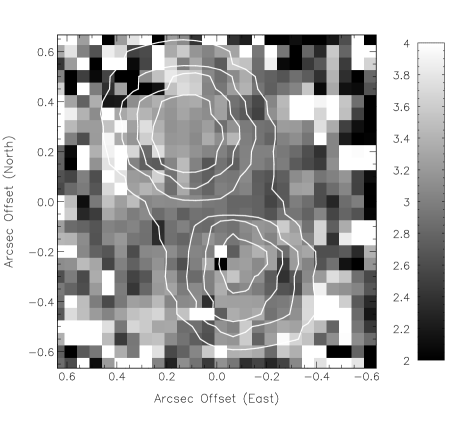
Figure 3: The ortho-para ratio image, calculated from the $1-0$ S(0,1,2) lines, superimposed with contours of K-band surface brightness (see Fig. 1) to indicate the location of the nebulosity.

4.3 Rotational and vibrational temperatures

In regions where shocks dominate, the level populations are expected to be thermalised, resulting in similar rotational and vibrational temperatures: $T_{\rm rot}\sim T_{\rm vib}$ (see Burton 1992 for a review). In UV-dominated regions, the higher vibrational levels (${\rm v}\geq 2$) are over-populated so that $T_{\rm vib}\gg T_{\rm rot}$. A comparison of the rotational and vibrational temperatures can therefore be used as an indication of the excitation mechanism (e.g. Tanaka et al. 1989).

A convenient graphical method to determine the gas temperature, $T_{\rm g}$, is to plot normalised column densities against upper level temperatures (e.g. Hasegawa et al. 1987; Martini, Sellgren & Hora 1997; Rudy et al. 2002):

$$\ln\left[\frac{N_{i}g_{(1,3)}}{N_{(1,3)}g_{i}}\right]T_{\rm g}=T_{i}-T_{(1,3)}$$ (2)

where $N_{i}$ is the column density of H₂ in the upper level, $i$, of a particular transition, and $N_{(1,3)}$ is the upper level column density for the $1-0$ S(1) line (${\rm v}=1,{\rm J}=3$). The respective statistical weights are $g_{i}$ and $g_{(1,3)}$ and we use the ortho-para ratio of 3.0 calculated in the previous section. In such a plot, $T_{\rm g}$ is given by the inverse of the slope of a line connecting the data points. We derive two estimates of the rotational temperature, $T_{\rm rot}$, for the $1-0$ and $2-1$ transitions, by fitting a line through transitions within the same vibrational level. The vibrational temperatures, $T_{\rm vib}$, are obtained by comparing ${\rm v}=2-1$ and ${\rm v}=1-0$ transitions with the same rotational quantum number, J. The column densities, $N_{i}$, are obtained from the line fluxes, $F_{i}$, in Table 1, where:

$$F_{i}=\frac{hcN_{i}E_{i}}{\lambda_{i}}10^{-0.4A_{i}}$$ (3)

with $\lambda_{i}$ the wavelength, $E_{i}$ the quadrupole transition probability (Turner, Kirby-Docken & Dalgarno 1977) and $A_{i}$ the extinction, for the line.

Figure 4: The log of the normalised column densities versus upper level temperature for the H₂ emission lines in Table 1. The upper plot is not corrected for extinction whereas the lower plot has an extinction correction of $A_{K}=1$ mag. applied. Separate fits to the ${\rm v}=1-0$ points [excluding $1-0$ S(3)] and ${\rm v}=2-1$ points are shown as solid black lines, and give estimates of $T_{\rm rot}$. A fit through the combined $1-0$ and $2-1$ data points [excluding $1-0$ S(3)] is shown by a dashed line. A fit through all the $1-0$ points is shown as a light black line.

Table 3: Rotational and vibrational temperatures calculated from the normalized column densities plotted in Fig. 4. Excluding the $1-0$ S(3) point the fits are consistent with $T_{\rm rot}\approx T_{\rm vib}$. A fit through all the data points gives the temperature, $T_{\rm g}$, that the gas would have if characterized by a single excitation temperature.

Estimate	Temperature (K)
	$A_{K}=0$	$A_{K}=1$
$T_{\rm rot}$ ${\rm v}=1-0$	$1379\pm 226$	$1901\pm 431$
$T_{\rm rot}$ ${\rm v}=2-1$	$1805\pm 834$	$2320\pm 1378$
$T_{\rm vib}$ (J=3)	$2201\pm 202$	$2106\pm 185$
$T_{\rm vib}$ (J=4)	$2334\pm 570$	$2216\pm 514$
$T_{\rm g}$	$2053\pm 123$	$2128\pm 132$
$T_{\rm rot}$ ${\rm v}=1-0^{\dagger}$	$1155\pm 122$	$1468\pm 197$
$T_{\rm vib}$ (J=5)†	$3132\pm 522$	$2904\pm 449$
$\dagger$ fits including the $1-0$ S(3) point

We plot our data in Fig. 4, both with no extinction correction (top) and with a correction for a K-band ($\lambda=2.2~{}\mu$m) extinction of 1 mag. (lower), which is the maximum value consistent with the Q3/S1 ratio (Sec. 3.4). The extinctions at each transition wavelength, $A_{i}$, are extrapolated assuming a power-law relationship (see footnote 1). We note that the $1-0$ S(3) point, at an upper level temperature of 8365 K, appears rather low in these plots. Although the line appears strong in Fig. 2, its flux relative to the $1-0$ S(1) line is in fact much weaker than expected for shock-excited gas: from our data $1-0$ S(1)/$1-0$ S(3) = 2.21 whereas a C-shock model from Smith (1995) gives a ratio of 1.13. The $1-0$ S(3) line lies outside the K-band, at 1.96 $\mu$m, in a region of poor atmospheric transmission, and may therefore be subject to a poor telluric correction. In view of these doubts, we have performed fits to the data in Fig. 4 both including and excluding the $1-0$ S(3) line.

The solid black lines show weighted least-squares fits to the $1-0$ and $2-1$ data points, excluding the S(3) point, providing two estimates of $T_{\rm rot}$. Correcting for 1 mag. of extinction (lower panel) improves the fit, reducing the scatter on the $1-0$ data points. Increasing the extinction correction much beyond $A_{\rm K}=1$ starts to increase the scatter again. These fits indicate a rotational temperatue of $\approx 2000$ K within errors for the extinction corrected data (Table 3).

The three estimates of $T_{\rm vib}$ are formed by comparing the three ${\rm v}=2-1$ rotational levels with their ${\rm v}=1-0$ equivalents. The resulting temperatures and errors are given in Table 3. We can see that the vibrational temperature based on the $2-1$ S(3) and $1-0$ S(3) lines (J=5) appears anomalously high, which again casts doubt on our measured $1-0$ S(3) flux. In fact, a reasonable straight line fit can be made to all the data points if the $1-0$ S(3) point is excluded, and this is shown as a dashed line in Fig. 4. This would imply that $T_{\rm rot}\approx T_{\rm vib}$, which is typical of shock-excited gas (Tanaka et al. 1989).

4.4 Shock models

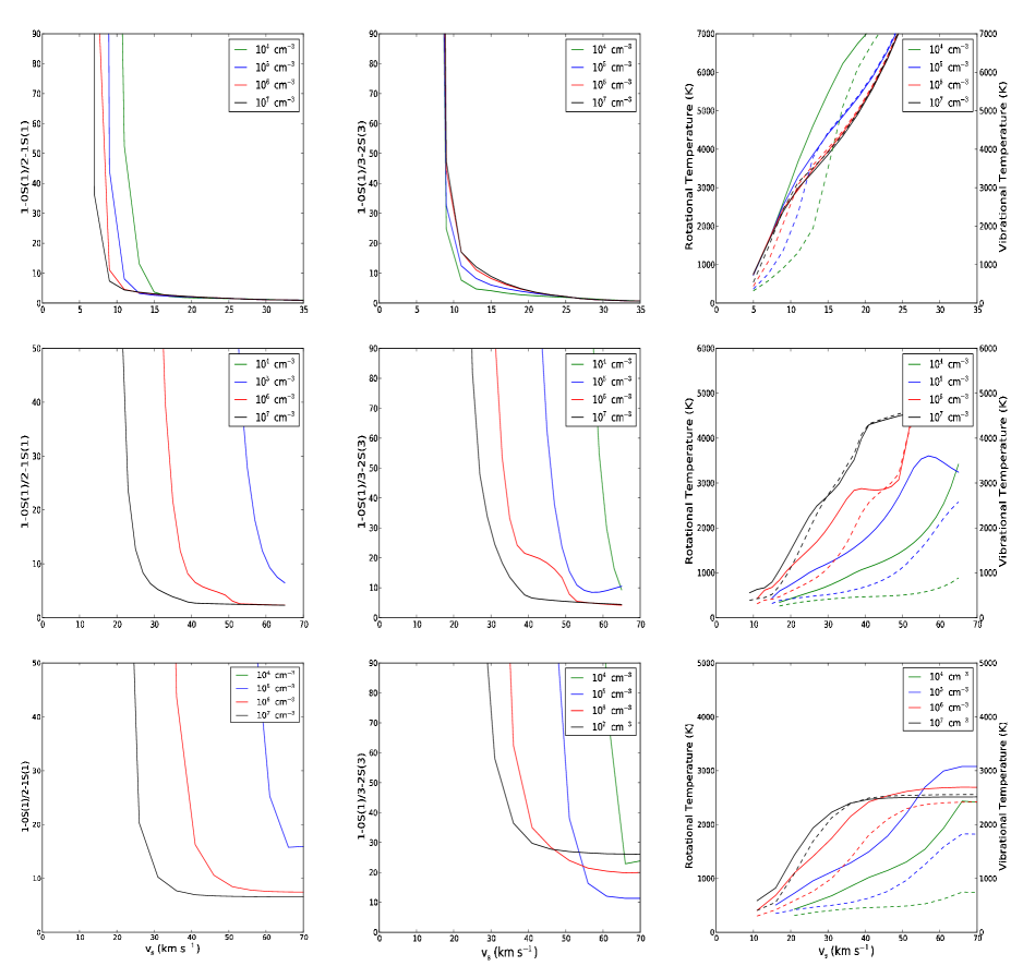
Figure 5: Model plots showing J-type planar (upper), C-type planar (middle) and C-type bow (lower) shocks. From left to right the panels show the $1-0$ S(1)/$2-1$ S(1) line ratio, the $1-0$ S(1)/$3-2$ S(3) line ratio and the excitation temperatures (rotational as solid lines and vibrational as dotted lines) as a function of shock velocity, and for a range of gas densities according to the legend in the inset boxes. See main text for further details. A colour version of this Figure is available online.

The velocity of the shock required to collisionally populate the ${\rm v}=2$ vibrational level depends on the density of the gas into which the shock propagates. For a planar C-shock with a transverse magnetic field (maximum cushioning) and a pre-shock gas density of $10^{7}$ cm^-3, a shock velocity of $\approx 20$ km s^-1 can produce the observed $1-0$ S(1)/$2-1$ S(1) line ratio of $\approx 10$ (Le Bourlot et al. 2002). SC07 estimate a gas density (based on dust optical depth) of $2-4\times 10^{7}$ cm^-3 in the limb-brightened edges and cap of the northern lobe, so that a shock in this velocity range could produce the observed H₂ emission in this region. These shocks, propagating into the cavity walls, may also contribute to the overall envelope expansion. Spatially unresolved ¹²CO ${\rm J}=1-0$ observations give an average envelope expansion velocity of 17 km s^-1 (SC07). This is similar to the 13 km s^-1 expansion velocity determined from OH maser observations (Bains et al. 2003), which trace the kinematics within a 1 arcsec radius of the star.

To further refine these arguments we calculate the expected line ratios [$1-0$ S(1) relative to $2-1$ S(1) and $3-2$ S(3)] and rotational and vibrational temperatures for various shock velocities and gas densities. We consider J- and C-type planar and curved (bow) shocks, using the models described by Smith, Kanzadyan & Davis (2003), Smith (1994), Smith & Brand (1990) and references therein. In the case of bow shocks, a paraboloidal shock is used with the shape characterised by a curvature exponent $s=2$ (see Smith et al. 2003). We assume that all of the hydrogen is in molecular form.

We find that planar J-shocks, Fig. 5 (upper), produce too much flux in the ${\rm v}=2$ and ${\rm v}=3$ lines to remain consistent with our observed line ratios, except for shock velocities less than 8 km s^-1. This velocity limit seems unreasonably low given the evidence for bulk motions of the molecular gas in excess of this figure, from CO and OH measurements, and the likelihood of a faster wind component (discussed in Section 7.1). This is also true of J-type bow shocks, although a velocity of up to 10 km s^-1 is allowed in this case. Higher velocity planar J-shocks will also raise the gas temperature to $\sim 3000$ K, which again is inconsistent with our line ratios.

C-shocks occur when a magnetic field cushions the shock in gas with a low pre-shock ionization fraction, typical of molecular clouds. If the ionization fraction exceeds $\sim 10^{-5}$ then a J-shock occurs (Smith 1994), however in the case of IRAS 18276 there is no evidence for an ionized region. The detection of Zeeman-split OH maser components in the equatorial regions of IRAS 18276 argues for a magnetic field of a few mG in these regions (Bains et al. 2003). Taking $B=4$ mG, then for a gas density of $10^{7}$ cm^-3, the Alfvén speed is $V_{a}\approx 2$ km s^-1 [given by $V_{a}=1.85\times 10^{3}B({\rm mG})n({\rm cm}^{-3})^{-0.5}$ km s^-1; e.g. Smith 1994]. The C-shock models for $V_{a}=2$ km s^-1 are shown in Fig. 5 (middle) and (lower) for planar and bow shock respectively. A common characteristic of the C-shocks is that they predict significantly different rotational and vibrational temperatures, irrespective of shock velocity, for all but the highest density ($10^{7}$ cm^-3) gas. We observe $T_{\rm rot}\approx T_{\rm vib}$ within errors, so that our data are consistent with the high density C-shock models. Taking $n=10^{7}$ cm^-3, then our line ratios constrain the shock velocity to $\approx 25$ km s^-1 for a planar shock and $\approx 30$ km s^-1 for a bow shock. These velocities result in gas temperatures of $\approx 2000$ K, again as observed. This argument is somewhat contingent on our assumption that all of the hydrogen is in molecular form. If we allow 20 per cent of the hydrogen nuclei to be in atomic form, then similar rotational and vibrational temperatures are achieved for all densities ($10^{4}-10^{7}$ cm^-3) in our models. However, as mentioned above, there is evidence for densities $\sim 10^{7}$ cm^-3 in the cavity walls, where material is swept up. Under these conditions hydrogen molecules should (re)form on dust grains on a timescale of $<100$ yr (Smith et al. 2003), so the assumption of fully molecular hydrogen in the dense pre-shock gas seems justified.

To summarize, our line ratios indicate that the H₂ emission arises in C-shocks in dense ($>10^{7}$ cm^-3) gas. At these densities and with a transverse magnetic field of 4 mG, a shock velocity in the range $25-30$ km s^-1 is consistent with observation.

5 Distribution of H₂ emission

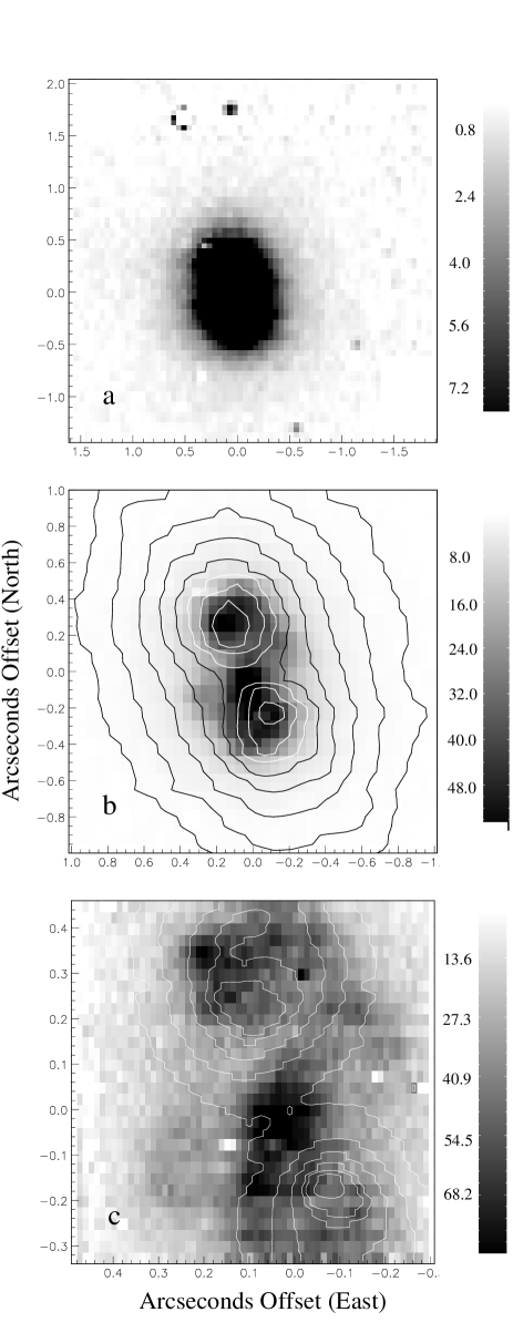
Figure 6: Images of the $1-0$ S(1) emission in a format similar to that of the K-band continuum emission (Fig. 1). The entire field, showing the faint emission, is seen in the MRM image in (a) with the brighter central emission shown on an expanded spatial scale in (b). The HRM $1-0$ S(1) image is shown in (c). Greyscale units are $\times 10^{-18}$ W m^-2 arcsec^-2. The H₂ emission in (b) and (c) is superimposed with contours of the MRM and HRM K-band continuum emission, respectively, with contour levels identical to those in Fig. 1.

The spatial distribution of the H₂ emission lines can be investigated by collapsing the continuum-subtracted datacube over the width of a line, to form an image of the line emission. This is shown for the brightest H₂ line, the $1-0$ S(1) line, in Fig. 6. The format is the same as for Fig. 1, which shows the distribution of the continuum emission. Firstly, in Fig. 6a, we see that the field star to the north-west of IRAS 18276 has disappeared, as expected if the continuum subtraction is successful. Secondly, the H₂ emission appears more centrally concentrated than the K-band continuum (Fig. 1), and not as elongated. There is no evidence for the searchlight beams, seen clearly in the continuum, confirming that these are scattered light features. At higher brightness contrast (Fig. 6b) we clearly see H₂ emission emanating from the vicinity of the bipolar lobes, but we also see emission in the equatorial region between the lobes, where the continuum contours pinch in due to the high optical depth of the circumstellar torus. In particular, there is a bright spot of H₂ emission located close to the centre of this region. The distribution of H₂ is therefore quite different from that of the scattered light. The other $1-0$ S- and Q-branch lines show a very similar brightness distribution, with a central bright spot, emission from the lobe regions and fainter emission from the equatorial region. The $2-1$ S-branch lines (not shown) have the same overall appearance as the $1-0$ lines. We have analysed the $1-0$ S(1)/$2-1$ S(1) flux ratio in the lobe regions and in the equatorial regions and find no significant difference within errors, suggesting that the shock characteristics are similar in these regions.

The HRM image of the $1-0$ S(1) emission over a field of view of $0.8\times 0.8$ arcsec is shown in Fig. 6c, with HRM continuum contours superimposed. At this spatial resolution (FWHM $\sim 70$ mas) the H₂ emission in the nebular lobes is seen to be clumpy, with a patch of emission to the north-east of the continuum peak in the north lobe. In the south lobe, the brightest H₂ emission runs down the east side of the lobe, again avoiding the continuum peak. This region coincides with the reddest colours in the $M_{s}-L_{p}$ map of SC07 (their fig. 11) which suggests that the H₂ emission arises within the dense shocked interface layer between the cavity and the surrounding envelope. This interpretation is consistent with the high-density C-shock models presented in Section 4.4.

The differentiation between the scattered light and H₂ emission is most noticeable in the equatorial regions. We see a bright, diffuse patch of H₂ emission in the centre of the obscuring lane (Fig. 6c). The circumstellar optical depth to the star along this line of sight at 2.12 $\mu$m is estimated to be $\tau_{2.12}>12.3$ (SC07), so that the H₂ emitting region must be in front of the star. Its appearance is again similar to the shape of the $M_{s}-L_{p}$ colour contours, suggesting that the emission arises from shocks within the walls at the base of the cavity lobes, which are only just starting to be penetrated by stellar photons in the $M_{s}$ image (SC07).

Surrounding the central patch, we see an elliptical or ring-like region of H₂ emission, with a semi-major axis of 0.29 arcsec, oriented at PA 112°. The orientation is similar to that of the faint equatorial structure seen in the $L_{p}$-band image of SC07, radius 0.6 arcsec, which they interpret as the outer parts of an equatorial torus. These authors also fit the SED with a two-shell dust model which has a density discontinuity at a radius of $1.6\times 10^{16}$ cm from the star, corresponding to a sudden drop in mass-loss rate from $\sim 2\times 10^{-3}$ to $\sim 3\times 10^{-5}$ M_⊙ yr^-1 at the end of the AGB. The distance to IRAS 18276 is uncertain, but OH maser phase-lag measurements combined with VLA interferometry (Bowers, Johnston & Spencer 1983) indicate that it lies between 3.4 and 5.4 kpc. Assuming a distance of 4 kpc to IRAS 18276 (Section 8.4), then this density discontinuity has an angular offset of $\approx 0.27$ arcsec from the star, which coincides with our equatorial H₂ emission. We propose that this ring of emission is produced in a shock at the inner boundary of the AGB envelope.

If we assume that the deprojected equatorial H₂ distribution is in fact circular, then the measured eccentricity of 0.86 corresponds to a tilt of the polar axis of this equatorial structure by $\approx 22$°. relative to the plane of the sky. The PA of this axis, at 25°, lies close to the bipolar axis defined by the continuum peaks (PA = 24°; Section 3.1) and to the illumination axis determined from near-infrared polarimetry (PA = 23°; Gledhill 2005).

6 CO bandheads

Figure 7: The continuum-subtracted spectrum in the first CO overtone region showing the first 4 bandheads in emission (upper) with an expanded view of the ${\rm v}=2-0$ bandhead (lower).

Between 2.29 $\mu$m and the H₂ Q-branch transitions longward of 2.4 $\mu$m, the K-band spectrum is dominated by the first overtone ro-vibrational transitions of CO. In Fig. 7 we show the continuum-subtracted spectrum in this region. The ${\rm v}=2-0$ bandhead is clearly in emission, with evidence for emission in the ${\rm v}=3-1$, $4-2$ and $5-3$ bandheads also. Beyond $\sim 2.31~{}\mu$m the individual ${\rm v}=2-0$ rotational transitions are resolved in our data and are seen to go into absorption (roughly at J = 23). We estimate the emitted flux in the $2-0$ bandhead between 2.293 and 2.306 $\mu$m to be $4.66\pm 0.37\times 10^{-17}$ W m^-2. The peak of the bandhead lies at 2.2948 $\mu$m, which is a shift of $1.315\times 10^{-3}~{}\mu$m redward of the rest wavelength, $\lambda_{o}=2.2935~{}\mu$m. The lower J (${\rm v}=2-0$ R-branch) transitions (in absorption) extend across the ${\rm v}=3-1$ bandhead [R(0) is at $\sim 2.347~{}\mu$m in our data] so that it is not possible to reliably estimate the flux in this bandhead. Similarly, the P-branch extends across the ${\rm v}=4-2$ bandhead .

The continuum-subtracted datacube has been collapsed in wavelength between 2.2926 and 2.3061 $\mu$m to form an image of the emission in the ${\rm v}=2-0$ bandhead, which is shown in Fig. 8 superimposed with contours of the K-band white light image from Fig. 1b. Unlike the distribution of H₂ emission, the distribution of CO emission is indistinguishable from that of the continuum, which is dominated by scattered light. As the continuum subtraction in this spectral region is difficult, we have examined the individual wavelength channels in the continuum-subtracted datacube to ensure that the subtraction is successful and that the resulting CO image is not contaminated with continuum emission. We are confident that Fig. 8 shows the distribution of the CO bandhead emission. The fact that the CO emission has the same spatial distribution as the scattered continuum suggests that it too originates close to the central object and is scattered into our line of sight by dust in the walls of the polar cavities. We can therefore predict that spectropolarimetry of the CO feature would reveal it to have the same high degree of linear polarization as the continuum at that wavelength. We find no difference in the bandhead profiles between the northern and southern lobes and in both cases the peak of the ${\rm v}=2-0$ bandhead lies at $2.2948~{}\mu$m, red-shifted relative to the rest wavelength.

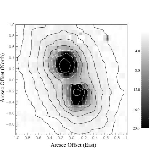
Figure 8: A continuum-subtracted image of the ${\rm v}=2-0$ bandhead emission superimposed with K-band continuum contours (Fig. 1b), showing that the distribution of CO emission is indistinguishable from that of the scattered continuum. Greyscale levels are in units of $10^{-18}$ W m^-2 arcsec^-2.

First overtone CO emission has been widely reported in young stellar objects (YSOs), where the emission is thought to arise from dense ($n>10^{10}$ cm^-3) regions of molecular gas at temperatures in the range 2000-5000 K (e.g. Scoville et al. 1979; Scoville et al. 1983). In these sources the gas is likely to reside in a circumstellar accretion disc close to the YSO and modelling of the bandhead profiles and strengths is in some cases consistent with emission produced in a Keplerian disc located within a few AU of the star (e.g. Carr 1989; Bik & Thi 2004).

Our results are consistent with the CO overtone emission being excited in a compact region close to the star. The distribution of the emission and of the continuum is indistinguishable (Fig. 8), indicating that both originate from an unresolved central source. This source is completely obscured from direct view in the near-IR by the optically thick dust torus and is instead seen reflected by dust grains in the polar lobes. The ${\rm v}=2-0$ bandhead profile shown in Fig. 7 is remarkably similar to the profiles observed in a number of YSOs, especially those modelled with low-inclination (i.e. close to pole-on) circumstellar discs (e.g. Chandler, Carlstrom & Scoville 1995; Bik & Thi 2004). In these YSO models the CO is collisionally excited in a disc around the star with temperature in the range 3000-4000 K and densities $n\geq 10^{10}$ cm^-3. Radiative excitation mechanisms (pumping by UV or IR photons) do not yield the observed rotational distributions or bandhead ratios (Scoville et al. 1979; Scoville, Krotkov & Wang 1980; Carr 1989). Comparing our $2-0$ bandhead spectrum with the model spectra of Scoville et al. 1983, for the BN object, the best match is for an optically thin line model, with an excitation temperature of 3500 K and velocity broadening of between 50 and 100 km s^-1. However, collisional excitation under these conditions would be expected to produce a $3-1$ bandhead that is at least as strong as the $2-0$ bandhead (e.g. Kraus et al. 2000) and this is generally what is observed in both YSO and post-AGB CO overtone emitters (see references above). This is clearly not the case for IRAS 18276, although as mentioned above, the ${\rm v}=3-1$ bandhead is strongly affected by the lower ${\rm v}=2-0$ rotational transitions which are in absorption, so that the $3-1$ flux appears much reduced. This effect is also seen to some extent in the BN object spectrum (Scoville et al. 1983) where cooler gas along the line of sight is thought to be responsible, and in transient CO emission observed in the yellow hypergiant $\rho$ Cas (Gorlova et al. 2006).

A further signature seen in YSO spectra, indicating rotating discs, is the presence of a blue wing or splitting of the bandhead peak into blue- and red-shifted components, depending on the inclination of the disc to the line of sight (e.g. Chandler et al. 1995; Najita et al. 1996). These features are not evident in our data, however, our view of the central region is provided by dust grains close to the polar axis so that if a central rotating disc is present (and assuming that its major axis lies close to the nebular axis) it would be viewed close to pole-on. We therefore cannot rule out rotation of any central disc. Similarly, we cannot determine from these data whether the gas in the disc is infalling or outflowing, however its presence within a few stellar radii of the source is a strong signature of ongoing mass loss.

7 Velocity structure

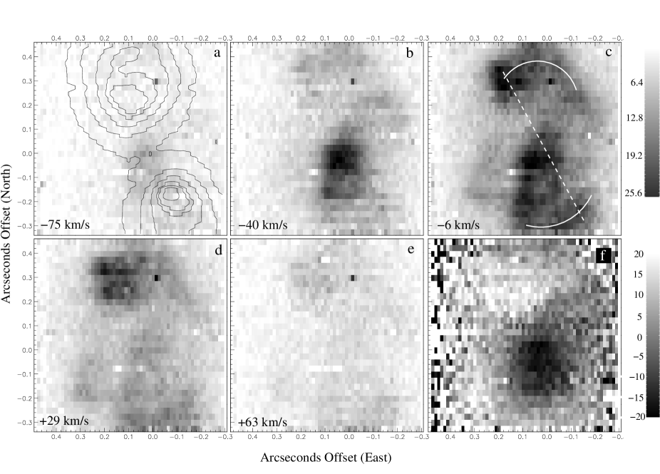
Figure 9: Panels (a) to (e) show ‘channel maps’ from the HRM datacube across the $1-0$ S(1) line, labelled with the velocity at the centre of the channel (relative to a systemic velocity of 61.5 km s^-1). Each image is displayed at the same greyscale range as indicated by the scale to the right of panel (c) in units of $10^{-18}$ W m^-2 arcsec^-2. Panel (a) also shows K-band continuum contours. Panel (f) shows a position-velocity map of the $1-0$ S(1) emission obtained by Gaussian-fitting the emission line. The greyscale units are km s^-1 relative to systemic. In panel (c) we also mark two arcs of emission along with an axis joining the bright emission patch in the northern lobe to an emission patch in the southern lobe. These features are discussed further in Section 8.4.

Information on the velocity structure of the molecular gas can be obtained from the SINFONI spectral cubes even though the velocity resolution is quite coarse, with the width of a spectral pixel (channel) corresponding to $34.6$ km s^-1 at 2.122 $\mu$m. The SINFONI user manual quotes a FWHM in the spectral direction of 2 pixels in the K-band, although investigation of the arc lines suggests that the total width of the spectral profile can be broad, with the line emission spread over as much as 10 pixels in the wavelength direction. The accuracy of the wavelength calibration is a further possible source of error when determining velocities, so we have checked this by matching atmospheric absorption features in the science data against a high spectral resolution atmospheric template to determine and correct for any offset.

The systemic velocity of IRAS 18276 is $V_{\rm LSR}=61.45\pm 0.18$ km s^-1 as determined from OH maser observations (Bains et al. 2003) which is in agreement with $V_{\rm LSR}=62$ km s^-1 determined from the ¹²CO $J=1-0$ line centre (SC07).

7.1 ${\rm v}=2-0$ CO bandhead

The ${\rm v}=2-0$ ¹²CO bandhead peak lies at 2.9848 $\mu$m relative to the rest wavelength of 2.2935 $\mu$m, equivalent to a LSR-corrected velocity of $V_{\rm LSR}=156\pm 15$ km s^-1 or $V_{\rm rel}=95\pm 15$ km s^-1 relative to the systemic velocity of 61.45 km s^-1. The error on our velocity corresponds to half a spectral pixel at the wavelength of the CO bandhead, so is a conservative estimate. As mentioned in Section 6, the distribution of CO emission is indistinguishable from that of the scattered continuum, and we measure the same red-shifted relative velocity in both the north and south lobes. We interpret this red shift as the radial velocity (from the star), along the polar axis, of the dust grains responsible for scattering the CO emission. In other words, assuming that the bandhead emitting region is an unresolved, centrally located source, obscured from direct view (as described in Section 6) moving at the systemic velocity, we can use the peak emission wavelength of the reflected bandhead to estimate the velocity of the dust in the axial outflow, $V_{\rm axial}=95\pm 15$ km s ^-1.

7.2 H₂ emission

As noted earlier, the distribution of H₂ emission differs considerably from that of the scattered continuum, and its velocity structure can be investigated by examining slices through the SINFONI datacube (channel maps). Fig. 9, panels (a) to (e), shows 5 slices through the $1-0$ S(1) line taken from the HRM cube, representing contiguous 34 km s^-1-wide spectral pixels, with the central velocity (relative to systemic) shown in each panel (negative velocities are blue shifted). As mentioned above, the FWHM in the spectral direction is at least 2 channels, however there is clearly velocity structure in the emission. Little emission is seen in the extreme velocity channels, (a) and (e), and what there is probably results from the spectral PSF. The central bright patch of H₂ emission is prominent in panels (b) and (c), but absent in (d), showing that this region has a blue-shifted component. Conversely, the bright patch in the northern lobe is prominent in panels (c) and (d), but absent in (b), indicating that it has a red-shifted component. The faint equatorial structure to the east of the star also appears more red than blue shifted, as does the southern lobe, as seen at the lower edge of the field in panel d. Panel (f) shows a position-velocity map of the emission, generated by fitting Gaussian profiles in the spectral direction at each spatial pixel using the VELMAP application in the STARLINK software collection. This map therefore shows the velocity of the peak of the emission line at each position, and the central patch is clearly blue shifted relative to the systemic velocity, whereas the northern patch, eastern equatorial region and, to some extent the southern lobe, are red shifted. The same tendency for a blue-shifted central patch and red-shifted lobes is seen in all other $1-0$ S- and Q-branch lines. The effect is harder to see in the $2-1$ lines as these are intrinsically fainter.

If the central H₂ patch lies in front of the star (Section 5) then this is consistent with it being predominantly blue shifted; the emission in this region results from shocks in gas flowing mainly towards us. The far side (red-shifted component) of this outflow is not seen due to the high obscuration through the central region. The position-velocity diagram in Fig. 9f shows a line-of-sight velocity of up to -20 km s^-1 in this region. As the orientation of any outflow in this region is unknown, it is not possible to estimate the actual outflow velocity.

The red-shifted component in the northern lobe is harder to explain, especially as the relative continuum brightness of the northern and southern lobes suggest that the northern lobe is tilted slightly towards the observer (e.g. Gledhill 2005). It is possible that the red-shifted patch lies on the far side of the northern lobe and so has a line-of-sight velocity component away from the observer. It seems unlikely, however, that we are seeing emission preferentially from the far side of the lobe, given that our analysis in Section 4 indicates that the shocks are occurring in high density and hence optically thick regions. Alternatively, some of the H₂ emission may be scattered by dust grains flowing along the cavity, away from the H₂ emitting region, adding a red-shifted component to the velocity of the line. This would also impart a similar red shift to the emission from the southern lobe, as observed, so this would seem a viable explanation. To investigate these possibilities further will require observations with higher velocity resolution than that afforded by SINFONI. Also, polarimetry of the H₂ lines would help to determine whether there is a scattered component to the emission.

8 Further discussion

8.1 The central regions

Bedijn (1987) found that in order to fit the infrared SED of IRAS 18276 it was necessary to assume that mass loss did not cease abruptly at the end of the AGB, but instead continued at a decreasing rate. This leads to a region of warm dust interior to the AGB shell causing the excess flux seen in $2-6~{}\mu$m photometry. Emission from warm dust is also indicated by our K-band spectrum (Fig. 2) in which the continuum flux density rises by a factor of 2 between 1.95 and 2.45 $\mu$m. The SED fit of SC07 indicates a stellar temperature and luminosity of $T_{\rm eff}=7000$ K and $L=6400$ L_⊙ so that the photospheric emission would be expected to fall over this wavelength range. Their model also indicates that the continuum is composed of 20 per cent stellar light and 80 per cent emission from a warm circumstellar dust cloud and that both components suffer an extinction of $\tau_{2.12~{}\mu{\rm m}}\sim 3.7$. Taking these assumptions, our K-band continuum slope implies a blackbody temperature of $\sim 450$ K for the warm dust, which is within the range of $300-500$ K determined by SC07.

An alternative location for the dust could be in the lobes of the cavities, where we see bright continuum emission in our images, but it would not be possible for dust grains to achieve temperatures of $\sim 450$ K in equilibrium with the stellar radiation field at these offsets. Our H₂ imaging shows that shocks are being driven into the cavity walls with gas temperatures $\sim 2000$ K, so it is possible that dust could be heated by the shocks. However, the distribution of shocked H₂ emission is very different to that of the K-band continuum, which is also highly polarised and therefore scattered. The most logical explanation is that the warm dust exists in a compact central region, which may extend all the way in to the condensation radius at $\sim 10^{14}$ cm and that mass loss is ongoing.

This conclusion is reinforced by our observation of CO bandhead emission which reveals the existence of hot ($T>2000$ K) and dense ($n>10^{10}$ cm^-3) molecular gas in a compact central region. The most likely location for this collisionally excited gas is close to the star, and typically within a few stellar radii (e.g. Oudmaijer et al. 1995; Scoville et al. 1983), in an inner torus or wind. A distance of 4$R_{*}$ corresponds to $1.5\times 10^{13}$ cm and is again consistent with extrapolation of the gas temperatures and densities of the SC07 model inwards (their fig. 13). We also see absorption in the lower J lines of the ${\rm v}=2-0$ CO transition (Fig. 7) which we interpret as a region of cooler gas, lying between the hotter central regions and the observer. As the radiation from the central region is being scattered into our line of sight by dust in the bipolar lobes, this cooler gas is probably part of the general mass outflow along the bipolar axis.

We also note in Fig. 2 the detection of the Na I doublet in emission. This is further evidence for the presence of high-density gas in the central region. As in the case of the CO bandhead emission, the Na I line has the same spatial distribution as the continuum indicating that it is scattered. The Na I lines have been observed in pre-main sequence jet sources associated with Herbig-Haro Objects (e.g. HH34 IRS and HH26 IRS) particularly when CO bandhead emission is also present (Antoniucci et al. 2008). These authors suggest that the Na I emission may originate from low-ionization gas that lies closer to the star (and is hotter) than that responsible for the CO emission.

A photospheric temperature of $T_{\rm eff}=7000$ K is at odds with our non-detection of Br$\gamma$. Many F and G spectral type post-AGB stars show a prominent Br$\gamma$ absorption line (e.g. Hrivnak, Kwok & Geballe 1994), the line only disappearing completely for spectral types later than about mid-K (Wallace & Hinkle 1997). This may argue for a much cooler effective temperature for IRAS 18276, but it seems more likely that any stellar absorption features are obliterated by the strong K-band dust continuum.

8.2 CO bandhead emission from evolved stars

First overtone bandhead emission from CO has been noted in a number of evolved stars. K-band spectroscopy of 16 post-AGB targets by Hrivnak, Kwok & Geballe (1994) detected emission in 3 objects (IRAS 19114+0002, IRAS 22223+4327 and IRAS 22272+5435) which they suggest is circumstellar in origin. In the case of IRAS 22272+5435, the CO bandheads changed from emission to absorption within a 3 month period, which Hrivnak et al. (1994) interpret as evidence for sporadic mass loss. These three objects are known to be associated with multi-polar nebulosity revealed in scattered light at optical and infrared wavelengths (e.g. Ueta et al. 2000, Gledhill et al. 2001) which again suggests a link with time-varying outflows.

García-Hernández et al. (2002) detect CO emission in three post-AGB objects: IRAS 08005-2356, IRAS 17423-1755 and IRAS 10178-5958. IRAS 08005-2356 has limb brightened bipolar lobes in the V-band (Ueta et al. 2000). Spectroscopic observations of the H$\alpha$ and H$\beta$ lines show P-Cygni profiles which are interpreted as a fast (up to 400 km s^-1) wind from the star (Slijkhuis, Hu & de Jong 1991). These authors also report a near-infrared excess which is modelled as emission from hot dust close to the star. V- and I-band images of IRAS 17423-1755 (Ueta et al. 2000) show a remarkable S-shaped nebula with a pronounced central obscuring disc. A series of collimated axial jets and emission line knots (Borkowski, Blondin & Harrington 1997) provide evidence for episodic and on-going mass-loss (Riera et al. 2002). IRAS 10178-5958 is a highly collimated bipolar object with open lobes, a central obscuring disc and prominent H₂ emission (e.g. Hrivnak et al. 2008).

CO bandhead emission is reported in the post-AGB objects HD 170756 (AC Her) and HD 101584 (IRAS 11385-5517) by Oudmaijer et al. (1995) who also suggest that the emission originates either in a circumstellar disc or a dense outflow close to the star. CO bandheads are seen in emission in the bipolar pre-PN M 1-92 (Hora, Latter & Deutsch 1999; Davis et al. 2003) in which H₂ emission is seen from Herbig-Haro-like bow shocks along the bipolar jet axis (Bujarrabal et al. 1998).

It seems clear that CO bandhead emission is closely linked to on-going mass loss and the presence of a circumstellar disc. In some cases there is direct evidence for this mass loss in the form of jets and fast outflows (e.g. IRAS 17423-1755). However, many bipolar pre-PN do not show prominent CO features in the near-IR. AFGL 2688 (The Egg Nebula) is often considered to be a prototypical example of a pre-PN and shares many characteristics with IRAS 18276 (see Sec. 8.3) but CO bandheads have not been detected (Davis et al. 2003). IRAS 17150-3224 is a well-studied bipolar pre-PN and shows emission from shocked H₂ in the near-IR, but not from CO (Davis et al. 2003). We suggest that CO bandhead emission in pre-PN indicates an ongoing intense phase of outflow or jet activity linked with the presence of shocks in dense ($\sim 10^{10}$ cm^-3) molecular gas. Objects not exhibiting CO bandheads may be in a more quiescent phase.

8.3 Equatorial H₂ emission

The occurrence of equatorial H₂ structures in post-AGB objects is, so far, uncommon. The most notable example is the case of AFGL 2688, in which HST NICMOS observations show an equatorial region of $1-0$ S(1) emission comparable in extent with the size of the bipolar lobes at that wavelength (Sahai et al. 1998). The H₂ emission in AFGL 2688 also results from shock excitation with a line ratio of $1-0$ S(1)/$2-1$ S(1) = 11 averaged over the object (Hora & Latter 1994), equivalent within errors to our value of 9.4$\pm$3.2 for IRAS 18276. The shock nature and appearance of the H₂ structures in AFGL 2688 imply that high velocity gas makes its way out through the central dust cocoon, which blocks stellar photons in the K-band, to interact with the slower moving gas in the circumstellar envelope. Sahai et al. (1998) suggest that this higher velocity outflow may occur along channels in the dust cocoon.

In IRAS 19306+1407, a more evolved object with a B-type central star, the nebulosity has a bipolar configuration in the optical, with a denser equatorial torus becoming prominent in near-IR polarized light (Lowe & Gledhill 2007). These authors model the SED and scattered light using an axisymmetric envelope with equator-to-pole density contrast 7:1. H₂ emission is seen in the bipolar lobes of this object as well as in two arcs on either side of the star, coincident with the inner edges of the dust torus. The emission is best fitted by a combination of shock- and UV-excitation and there is evidence from the clumpy nature of the arcs that the wind is beginning to erode paths through the circumstellar torus (Lowe & Gledhill 2006).

The ring of equatorial H₂ emission in IRAS 18276 also appears to be produced in shocks at the inner edge of the denser AGB envelope, where the density drops by two orders of magnitude. In this object the density step is not yet visible in scattered light or thermal dust images, so that IRAS 18276 is perhaps an antecedent of the more evolved IRAS 19306+1407.

8.4 The bipolar outflow

The angular extent of the northern lobe, measured from the star to the polar ‘cap’ (Fig. 1c) is 0.625 arcsec (12.5 milliarcsec pixels). Assuming $D=4$ kpc (Section 5) and that the bipolar outflow lies in the plane of the sky, then the linear extent of the northern lobe is $3.7\times 10^{14}$ m. An axial wind with velocity 95 km s^-1 would take 125 yr to travel this distance, which provides a lower limit for the age of wind-carved bipolar cavities. The radial distribution of the dust density in the envelope around IRAS 18276 (modelled by SC07) indicates a period of increasing mass loss (from $\sim 2\times 10^{-4}$ to $\sim 2\times 10^{-3}$ M_⊙ yr^-1) commencing more than 2300 and ending $\sim 300$ years ago. This abrupt end to the heavy mass-loss phase signals the start of post-AGB evolution. Although uncertainties of a factor of 2 or more may be present in our estimate of the cavity lifetime, it seems certain that the bipolar cavities are young relative to the AGB envelope and that they started to form very soon after the heavy mass-loss phase terminated.

The patchy distribution of the H₂ emission was noted in Sec. 5, and seems brightest close to the walls and tips of the bipolar cavities, forming arcs of emission at the ends of the cavities (marked on Fig. 9c). These arcs may trace the shock fronts where the axial outflow hits the ends of the cavities, which appear to be still closed in the continuum images (which trace the dust). The shock characteristics are indicative of gas densities of the order $n=10^{7}$ cm^-3 which are typical of those in the cavity walls and tips (Sec. 4.4), so that this scenario seems plausible. The bright patch in the northern lobe is particularly noticeable. It is quite possible that the material in the cavity walls has a clumpy distribution, and that impingement of the axial wind on these clumps leads to the patchy nature of the emission in IRAS 18276; H₂ emission from clumpy structures is seen in the equatorial region of IRAS 19306+1407 (Lowe & Gledhill 2006) and spectacularly in the Helix planetary nebula (NGC 7293; Matsuura et al. 2009). Additionally, if the axial outflow is more confined and jet-like, it may result in H₂ ‘emission spots’ at the jet tips. We propose that such a collimated axial outflow or jet is operating and is currently aligned with the emission spot in the northern lobe. If this jet is precessing and has excavated the cavities then the arcs of emission may represent the recent locus of the jet tip. In Fig. 9c we mark a possible jet axis, drawn between the bright H₂ patch in the northern lobe and a fainter patch in the southern lobe. This axis lies at PA = 29°, which is inclined relative to the major axis of the cavities at PA = 24°, defined by the two K-band continuum peaks, and to the K-band polarimetric axis, PA = $22\pm 2$°(Gledhill 2005). The angle subtended at the star by the H₂ patch in the northern lobe is $24\pm 5$°.

9 Conclusions

Integral field spectroscopic observations of IRAS 18276-1431 are analyzed to determine the distribution, excitation and kinematics of H₂ and CO emission in the K-band. We summarize our conclusions as follows:

1. We detect the K-band ${\rm v}=1-0$ and ${\rm v}=2-1$ S-branch lines of H₂, as well as the ${\rm v}=1-0$ Q-branch. The $1-0$ S(1)/$2-1$ S(1) ratio is $9.3\pm 3.2$ over most of the object, which is typical of shock excited emission. Further evidence for shock excitation is provided by an ortho-para ratio of $3.02\pm 0.18$ and roughly equivalent vibrational and rotational excitation temperatures of $\approx 2000$ K. A marginal detection of the ${\rm v}=3-2$ S(3) line is again consistent with shocks and indicates that UV-pumped fluorescence does not contribute significantly to the H₂ emission. This accords with the proposed evolutionary status in which IRAS 18276-1431 has recently left the AGB, is now carving outflows into the AGB envelope via a fast wind, but is not yet hot enough to UV-excite its surroundings.

2. Comparison of the observations with shock models favours C-shocks, with either a planar or curved (bow) configuration, in high density ($>10^{7}$ cm^-3) gas with shock velocities of $25-30$ km s^-1. This is also consistent with the previous detection of a $\approx 4$ mG magnetic field in the torus region.

3. The distribution of H₂ emission differs considerably from that of the scattered continuum and implies a clumpy distribution of material in the walls and tips of the outflow cavities. We suggest that the H₂ emission in these regions is shock excited by a fast axial outflow impinging upon dense gas. A bright patch of emission in the northern lobe may provide evidence for an inclined axial jet.

4. A bright spot of H₂ emission is located between the bipolar lobes where the scattered continuum is a minimum, and must lie between us and the star. We interpret this as shocks driven by the wind as it impacts dense material at the base of the cavities. We also see H₂ emission in the equatorial region, to the east and west of the stellar position, which may form an equatorial ring with radius $\approx 0.3$ arcsec. The location corresponds to the inner edge of the AGB envelope, where the density changes by two orders of magnitude, so that the emission may arise in shocks in the boundary region between the two (AGB and post-AGB) winds.

5. The velocity structure of the H₂ lines shows that the central spot has a blue-shifted component with the peak shifted by $\approx-20$ km s^-1 relative to the systemic velocity. Conversely, the emission from the bipolar lobes and equatorial region appears red shifted by a similar amount. We suggest that the blue-shifted central spot results from approaching shock fronts in material foreground to the star. The red-shifted lobe emission may be due to a component of line scattering by dust grains in the axial outflow, receding from the shock.

6. The K-band spectrum of IRAS 18276-1431 shows a rising continuum and evidence for the presence of warm $\sim 450$ K dust, suggesting that mass loss and dust formation is ongoing in this object.

7. Further evidence for continuing mass-loss is provided by the first overtone ¹²CO ro-vibrational bandheads, which are observed in emission, which may signify the presence of a circumstellar disc of hot CO located close to the star. CO bandhead emission is observed in several other post-AGB sources, all with evidence of ongoing mass loss, circumstellar discs and collimated outflows/jets. Detection of the Na I doublet in emission further suggests the presence of high-density gas close to the star.

8. The CO bandhead emission has the same spatial distribution as the scattered K-band stellar continuum, indicating that it is also scattered by dust grains in the polar lobes. This further supports a central, unresolved, location for the CO emitting region. We use the red shift of the peak of the scattered ${\rm v}=2-0$ bandhead to estimate the radial velocity (from the star) of the dust grains responsible for the scattering, leading to an estimate for the axial velocity of dust in the outflow of $95\pm 15$ km s^-1. This in turn places a lower limit of 125 yr on the age of the bipolar cavities meaning that any fast wind must have turned on very soon after the cessation of AGB mass loss.

The overall picture of IRAS 18276 is one in which the central star has recently moved into the post-AGB phase. Mass loss continues in the form of a more tenuous and faster wind, which is now driving shocks in the surrounding molecular material. Further monitoring of the $K-$band spectrum will be useful to determine if the CO bandhead emission persists, which may indicate a stable region of hot molecular gas close to the star.

References

- Antoniucci (2008) Antoniucci S., Nisini B., Giannini T., Lorenzetti D., 2008, A&A, 479, 503
- Bains (2003) Bains I., Gledhill T.M., Yates J.A., Richards A.M.S., 2003, MNRAS, 338, 287
- Bedijin (1987) Bedijin P.J., 1987, A&A, 186, 136
- Bik (2004) Bik A., Thi W.F., 2004, A&A, 427, L13
- Black (1976) Black J.H., Dalgarno A., 1976, ApJ, 203, 132
- Bonnet (2004) Bonnet H., et al., 2004, The ESO Messenger, 117, 17
- Borkowski (1997) Borkowski K.J., Blondin J.M., Harrington J.P., 1997, ApJ, 482, L97
- Bowers (1983) Bowers P.F., Johnston K.J., Spencer J.H., 1983, ApJ, 274, 733
- Bujarrabal (1998) Bujarrabal V., Alcolea J., Sahai R., Zamorano J., Zijlstra A.A., 1998, A&A, 331, 361
- Burton (1992) Burton M.G., 1992, Aust. J. Phys., 45, 463
- Burton (1990) Burton M.G., Hollenbach D.J., Tielens A.G.G.M., 1990, ApJ, 365, 620
- Carr (1989) Carr J.S., 1989, ApJ, 345, 522
- Chandler (1995) Chandler C.J., Carlstrom J.E., Scoville N.Z., 1995, ApJ, 446, 793
- Chrysostomou (1993) Chrysostomou A., Brand P.W.J.L., Burton M.G., Moorhouse A., 1993, MNRAS, 265, 329
- Davis (2003) Davis C.J., Smith M.D., Stern L., Kerr T.H., Chiar J.E., 2003, MNRAS 344, 262
- Davis (2005) Davis C.J., Smith M.D., Gledhill T.M., Varricatt W.P., 2005, MNRAS 360, 104
- Eisenhauer (2004) Eisenhauer F., et al., 2003, SPIE, 4841, 1548
- Garcia (2002) García-Hernández D.A., Manchado A., García-Lario P., Domínguez-Tagle C., Conway G.M., Prada F., 2002, A&A, 387, 955
- Gledhill (2005) Gledhill T.M., 2005, MNRAS, 356, 883
- Gledhill et al. (2001) Gledhill T.M., Chrysostomou A., Hough J.H., Yates J.A., 2001, MNRAS, 322, 321
- Gorlova et al. (2006) Gorlova N., Lobel A., Burgasser A.J., Rieke G.H., Ilyin I., Stauffer J.R., 2006, ApJ, 651, 1130
- Hasegawa (1987) Hasegawa T, Gatley I., Garden R.P., Brand P.W.J.L., 1987, ApJ, 318, L77
- Hollenbach (1995) Hollenbach D.J., Natter A., 1995, ApJ, 455, 133
- Hora (1994) Hora J.L., Latter W.B., 1994, ApJ, 437, 281
- Hora (1997) Hora J.L., Latter W.B., Deutsch L.K., 1999, ApJS, 124, 195
- Hrivnak et al. (1994) Hrivnak B.J., Kwok S., Geballe T.R., 1994, ApJ, 420, 783
- Hrivnak et al. (2008) Hrivnak B.J., Smith N., Su K.Y.L., Sahai R., 2008, ApJ, 688, 327
- Kastner (1996) Kastner J.H., Weintraub D.A., Gatley I., Merrill K.M., Probst R.G., 1996, ApJ, 462, 777
- Kelly (2005) Kelly D.M., Hrivnak B.J., 2005, ApJ, 629, 1040
- Kraus (2000) Kraus M., Krügel, Thum C., Geballe T.R., 2000, A&A, 362, 158
- Le Bourlot et al. (2002) Le Bourlot J., Pineau des Forêts G., Flower D.R., Cabrit S., 2002, MNRAS, 332, 985
- Lee (2009) Lee C.-F., Hsu M.-C., Sahai R., 2009, ApJ, 696, 1630
- Lowe (2006) Lowe K.T.E., Gledhill T.M., 2006, Planetary Nebulae in our Galaxy and beyond, eds. M.J. Barlow & R.H. Méndez, IAU Symp No. 234, p451
- Lowe (2007) Lowe K.T.E., Gledhill T.M., 2007, MNRAS, 374, 176
- Martini (1997) Martini P., Sellgren K., Hora J.L., 1997, ApJ, 484, 296
- Matsuura (2009) Matsuura M, et al., 2009, ApJ, 700, 1067
- Najita (1996) Najita J, Carr J.S., Glassgold A.E., Shu F.H., Tokunaga A.T., 1996, ApJ, 462, 919
- Oudmaijer et al. (1995) Oudmaijer R.D., Waters L.B.F.M., van der Veen W.E.C.J., Geballe T.R., 1995, A&A, 299, 69
- Ramsey (1993) Ramsey S.K., Chrysostomou A., Geballe T.R., Brand P.W.J.L., Mountain M., 1993, MNRAS, 263, 695
- Riera (2003) Riera A., García-Lario P., Manchado A., Bobrowsky M., Estalellar R., 2003, A&A, 401, 1039
- Rudy (2001) Rudy R.J., Lynch D.K., Mazuk S., Puetter R.C., Dearborn D.S.P., 2001, AJ, 121, 362
- Sahai (1998) Sahai R., Trauger J.T., 1998, A.J., 116, 1357
- Sahai et al. (1998) Sahai R., Hines D.C., Kastner J.H., Weintraub D.A., Trauger J.T., Rieke M.J., Thompson R.I., Schneider G., 1998, ApJ, 492, L163
- Sahai (2007) Sahai R., Morris M., Sánchez Contreras C., Claussen M., 2007, A.J., 134, 2200
- Sanchez Contreras (2007) Sánchez Contreras C., Le Mignant D., Sahai R., Gil de Paz A., Morris M., 2007, ApJ, 656, 1150
- Scoville (1979) Scoville N.Z., Hall D.N.B., Klienmann S.G., Ridgway S.T., 1979, ApJ, 232, L121
- Scoville (1980) Scoville N.Z., Krotkov R., Wang D., 1980, ApJ, 240, 929
- Scoville (1983) Scoville N.Z., Klienmann S.G., Hall D.N.B., Ridgway S.T., 1983, ApJ, 275, 201
- Siodmiak (2008) Siódmiak N., Meixner M., Ueta T., Sugerman B.E.K., Van de Steene G.C., Szczerba R., 2008, ApJ, 677, 382
- Slijkhuis (1991) Slijkhuis S., Hu J.Y., de Jong T., 1991, A&A, 248, 547
- Smith0 (1990) Smith M.D., Brand P.W.J.L., 1990, MNRAS, 242, 495
- Smith1 (1994) Smith M.D., 1994, MNRAS, 266, 238
- Smith2 (1995) Smith M.D., 1995, A&A, 296, 789
- Smith5 (1997) Smith M.D., Davis C.J., Lioure A., 1997, A&A, 327, 1206
- Smith3 (2003) Smith M.D., Khanzadyan T., Davis C.J., 2003, MNRAS, 339, 524
- Shull (1978) Shull J.M., Hollenbach D.J., 1978, ApJ, 220, 525
- Stead (2009) Stead J.J., Hoare M.G., 2009, MNRAS, 400, 731
- Tanaka (1989) Tanaka M., Hasegawa T., Hayashi S.S., Brand P.W.J.L., Gatley I., 1989, ApJ, 336, 207
- Turner (1977) Turner J., Kirby-Docken K., Dalgarno A., 1977, ApJS, 35, 281
- Ueta (2000) Ueta T., Meixner M., Bobrowsky M., 2000, ApJ, 528, 861
- Wallace (1997) Wallace L., Hinkle K., 1997, ApJS, 111, 445