Numerical simulations of wave propagation in the solar chromosphere

Abstract

We present two-dimensional simulations of wave propagation in a realistic, non-stationary model of the solar atmosphere. This model shows a granular velocity field and magnetic flux concentrations in the intergranular lanes similar to observed velocity and magnetic structures on the Sun and takes radiative transfer into account.

We present three cases of magneto-acoustic wave propagation through the model atmosphere, where we focus on the interaction of different magneto-acoustic wave modes at the layer of similar sound and Alfvén speeds, which we call the equipartition layer. At this layer acoustic and magnetic mode can exchange energy depending on the angle between the wave vector and the magnetic field vector.

Our results show that above the equipartition layer and in all three cases the fast magnetic mode is refracted back into the solar atmosphere. Thus, the magnetic wave shows an evanescent behavior in the chromosphere. The acoustic mode, which travels along the magnetic field in the low plasma-$\beta$ regime, can be a direct consequence of an acoustic source within or outside the low-$\beta$ regime, or it can result from conversion of the magnetic mode, possibly from several such conversions when the wave travels across a series of equipartition layers.

1 Introduction

Classical helioseismology relies on waves with frequencies below the acoustic cut-off frequency. These type of waves are trapped inside the acoustic cavity of the Sun. High frequency waves above the acoustic cut-off frequency, however, are able to travel freely into the solar atmosphere. Along their path through the atmosphere these waves interact with the complex magnetic field that is present in the photosphere and the chromosphere. Being able to observe these running waves in the atmosphere with high cadence instruments like MOTH (Finsterle et al., 2004a) a new field in helioseismology is emerging. However, the analysis tools at hand are still very basic (Finsterle et al., 2004b; Haberreiter et al., 2007) and the characterization of the interaction of the magneto-acoustic waves with the magnetic field is still difficult. For the interpretation of the observations, it is helpful to look at numerical simulations of wave propagation through a magnetically structured solar model atmosphere. In the past such simulations have always been carried out for idealized atmospheric models and magnetic configurations (Rosenthal et al., 2002; Bogdan et al., 2003). However, in reality the magnetic field is expected to have a complex structure.

Here we report on two-dimensional simulations of magneto-acoustic wave propagation in a model of the solar atmosphere including realistic granular velocity fields and complex magnetic fields. In Sect. 2 we will give a short description of the setup of the atmospheric model and of the excitation of the waves. In Sect. 3 we will present and discuss snapshots of our wave propagation simulations. Results are summarized in the last section.

2 Method

For the simulations of magneto-acoustic wave propagation, we carry out two-dimensional numerical experiments with the CO⁵BOLD code. The code solves the magnetohydrodynamic equations for a fully compressible gas including radiative transfer. Thus, the model atmosphere shows a realistic granular velocity field and magnetic flux concentrations in the intergranular lanes caused by the advective motion of the granules. More details on the application of the the CO⁵BOLD code for wave propagation experiments can be found in Steiner et al. (2007).

2.1 Two-dimensional model of the solar atmosphere

The model atmosphere used for the two-dimensional numerical wave propagation experiments is basically the same as was used by Steiner et al. (2007). The computational domain of the box covers the upper layer of the convection zone from about $-1\,300$ km below mean optical depth unity all the way to the middle layers of the chromosphere at about 1 600 km above mean optical depth unity. Along the vertical direction an adaptive grid with 188 grid points is used corresponding to cell sizes of 46 km for the biggest cells in the convection zone and 7 km for the smallest cells in the chromosphere. Transmitting boundary conditions are applied for the lower and upper boundary. The lateral dimension of the box is 5 000 km, with a grid resolution of 123 grid points corresponding to a horizontal spatial resolution of 40 km. Periodic boundary conditions are applied in the lateral directions.

Figure 1 gives an impression of the magnetic setup.

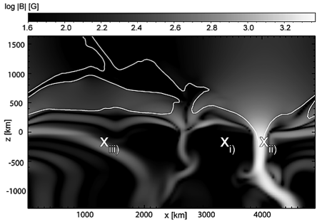
Figure 1: Magnetic setup of the model atmosphere represented in gray scales of $\log|B|$. The white curve corresponds to the equipartition layer. On the right hand side a flux sheet with strengths up to 2 300 G has evolved. On the left hand side in the photosphere are weak horizontal magnetic fields. The crosses indicate the location of the wave excitation, where the numbers correspond to the three cases mentioned in the text.

The plot shows the absolute magnetic field strength $\log|B|$. Since we are especially interested in the interaction of the waves with the magnetic field, we use a model where a strong flux sheet has evolved during the simulation time. In the core of the flux sheet, which is present on the right hand side of the box, magnetic field strengths up to 2 300 G are reached. On the left-hand side weaker horizontal fields have evolved. The white contour shows the equipartition layer where the Alfvén speed equals the sound speed, and approximately coincides with the $\beta=1$ layer. At this layer the acoustic and magnetic mode of the magneto-acoustic waves can exchange energy (Cally, 2007). This layer is known as the mode conversion zone, where an acoustic wave can change to a magnetic mode and vice versa. The strength of this interaction depends on the angle between the wave vector and the magnetic field (attack angle), the wave number $k$, and the width of the conversion zone (Cally, 2007). To investigate this interaction we excite waves at three different positions in the computational domain. The excitation positions are indicated by crosses in Fig. 1. The form of the excitation will be discussed in Sect. 2.2. The location of the excitation is at a depth for which it was shown that the excitation of waves in the Sun is most likely to take place namely between the surface and 500 km in depth (Stein & Nordlund, 2001). The three lateral positions are chosen at locations where interesting cases of wave and magnetic field interactions occur:

• where the magneto-acoustic waves interact with the magnetic canopy of the flux sheet,

• where the magneto-acoustic waves are excited inside the flux sheet, and

• where the magneto-acoustic waves interact with weak horizontal magnetic fields.

2.2 Wave excitation

In order to excite waves in our simulation domain we follow the description given by Parchevsky & Kosovichev (2009), where the spatial and temporal behavior of the wave source is modeled by the function:

$$f(r,t)\!=\!\begin{cases}A\left[\!1\!-\!\frac{r^{2}}{R^{2}_{\mathrm{src}}}\!\right]^{2}\!\!(1-2\tau^{2})\mathrm{e}^{-\tau^{2}}&\!\!\!\!\mbox{for }\,r\leq R_{\mathrm{src}},\\ 0&\!\!\!\!\mbox{for }\,r>R_{\mathrm{src}},\end{cases}$$ (1)

where

$$\tau=\frac{\omega_{0}(t-t_{0})}{2}-\pi\quad\mbox{with}\quad t_{0}\leq t\leq t_{0}+\frac{4\pi}{\omega_{0}},$$

$R_{\mathrm{src}}$ is the radius of the source, $A$ is the amplitude of the disturbance, and $\omega_{0}=2\pi f_{0}$ determines the central frequency of the wave excitation. This function can now be used as a source function in the momentum equations by taking the gradient of Eq. 1, $\vec{S}=\nabla f$. Then, the components of the source function $\vec{S}$ can be combined with the components of the pressure gradient. Thus, the source function can be seen as a perturbation to the pressure gradient, launching an acoustic wave with a central frequency of $\omega_{0}$.

For our simulations we use a central frequency of $f_{0}=20$ mHz and a radius of the source of $R_{\mathrm{src}}=50$ km. The temporal behavior of the wave source is plotted in panel a) of Fig. 2. The panel b) shows the power spectrum of the excitation source. A non-monochromatic wave is excited with most of the power around $f_{0}=20$ mHz.

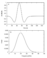
Figure 2: a) Temporal behavior of the wave source. b) Power of the wave source. The pressure disturbance excites a non-monochromatic wave with a central frequency of $f_{0}=20$ mHz.

3 Results

In this section we present snapshots taken from our simulations of wave propagation in a complex magnetically structured atmosphere. We will focus on the interaction between the wave and the magnetic field that is taking place in the mode conversion zone.

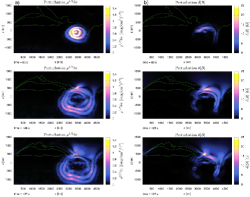
Figure 3: a) Perturbation of the square root of the energy density, $\rho^{1/2}\delta v$, caused by a wave that is excited outside in the vicinity of the flux sheet. Shown are three snapshots taken at 80 s, 126 s, and 137 s into the simulation run. b) Perturbation $\delta B$ of the magnetic field. The snapshots are taken at the same time as in panel a). In all plots, the solid contour corresponds to the equipartition layer indicating the conversion zone.

Panel a) of Fig. 3 shows snapshots of the propagation of a wave that is excited just outside of a flux sheet underneath the magnetic canopy. The propagation of both wave modes, the predominantly acoustic and predominantly magnetic mode, can be tracked in the perturbation of the square root of the energy density $\delta\epsilon^{1/2}=\rho^{1/2}\delta v$. Because of the position of the wave source beneath the $\beta=1$ layer, in a region of high plasma $\beta$, the applied wave source excites a wave that is predominantly an acoustic mode. Upon reaching the conversion zone, indicated by the solid contour in Fig. 3, energy is transferred from the acoustic to the magnetic mode (Cally, 2007). Because of the large attack angle between the local wave vector and the magnetic field vector, most of the energy is converted to the fast magnetic mode. Transmission of the acoustic mode is not apparent. The magnetic mode is best seen in the perturbation $\delta B$ of the magnetic field, plotted in panel b) of Fig. 3. The second plot in panel b), at 126 s into the simulation, shows the fast magnetic mode emerging from the conversion zone. Because of the gradient of the Alfvén speed, the wave is refracted back down into the photosphere.

Next, we will focus on the wave propagation when the wave source is located inside the flux sheet close to the equipartition layer. Figure 4 shows again snapshots of the perturbation of the square root of the energy density $\delta\epsilon^{1/2}$, panel a), and the perturbation $\delta B$ of the magnetic field, panel b). Since the wave source is located above the equipartition layer in the low-$\beta$ regime, the fast magnetic wave mode is excited directly and together with the slow acoustic mode, different from the previous case.

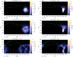
Figure 4: a) Perturbation $\delta\epsilon^{1/2}$ caused by a wave that is excited inside of the flux sheet close to the equipartition layer. Shown are three snapshots taken at 80 s, 105 s, and 180 s into the simulation run. b) Perturbation $\delta B$ of the magnetic field. The snapshots are taken at the same time as in panel a). In all plots, the solid contour corresponds to the equipartition layer indicating the wave-conversion zone.

Because of the higher Alfvén speed above the equipartition layer, the fast magnetic wave runs ahead of the slow acoustic mode. This fast magnetic mode can again be easily identified in the perturbation $\delta B$ of the magnetic field, plotted in panel b) of Fig. 4. As in the previous case, the gradient of the Alfvén speed causes the fast magnetic wave to refract to a degree that it travels back towards the lower atmosphere. The slow acoustic wave emerges from the location of the wave excitation at a later time (last plot in panel a) of Fig. 4), and is then guided along the magnetic field lines into the higher layer of the atmosphere. As the acoustic wave travels up the atmosphere the wave front is steepening and starts to shock.

Finally, we excite a wave just below weak horizontal magnetic fields. Snapshots of the wave propagation are plotted in Fig. 5, where panel a) shows again the perturbation of the square root of the energy density $\delta\epsilon^{1/2}$. Panel b) shows the perturbation of the pressure $\delta p/p_{0}$, with $p_{0}$ being the local unperturbed pressure.

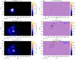
Figure 5: a) Perturbation $\delta\epsilon^{1/2}$ caused by a wave that is excited beneath weak horizontal magnetic fields. Shown are three snapshots taken at 80 s, 137 s, and 145 s into the simulation run. b) Perturbation of the pressure, $\delta p/p_{0}$. The snapshots are taken at the same time as in panel a). In all plots, the solid contour corresponds to the equipartition layer indicating the wave-conversion zone.

As the excitation location is below the equipartition layer in the high-$\beta$ regime, primarily the fast acoustic wave mode is excited. At the first equipartition layer, the local wave and magnetic vector are almost perpendicular to each other. Thus, most of the acoustic wave energy is converted into the fast magnetic mode. A transmitted acoustic wave is not visible at first. However, the existence of multiple equipartition layers in the path of the magneto-acoustic waves, adds to the complexity of the interpretation. Multiple equipartition layers have never been addressed in former investigations. Due to the large attack angle, one expects that no acoustic wave should be transmitted through the mode conversion zone. However, by looking at the pressure disturbance $\delta p/p_{0}$ in Fig. 5 it can be seen that an acoustic wave can be transmitted through the multiple equipartition layers by a series of mode conversion. In the middle plot of panel b) a strong pressure disturbance starts to reemerge above the multiple conversion zones. This can be seen as an indication of a transmitted acoustic wave in spite of the horizontal magnetic fields.

4 Summary

We have shown numerical experiments of wave propagation in a realistic two-dimensional model atmosphere. We focused on the interaction between acoustic and magnetic wave modes at the equipartition layer where the Alfvén speed is similar the sound speed.

When the location of the wave source is below the equipartition layer in the high-$\beta$ regime, the launched wave is predominantly acoustic in nature. In the first and third of the presented cases, the large attack angle of the local wave vector with the magnetic field vector results in the conversion of the fast acoustic mode into the fast magnetic mode. When there are multiple equipartition layers, an acoustic mode can be transmitted into the higher layers of the atmosphere by a series of mode conversions. In all three cases the fast magnetic mode is usually refracted back towards the lower atmosphere because of the gradient in Alfvén speed.

If the location of the wave source is close to the equipartition layer, both, the acoustic and the magnetic mode, are excited. The slow acoustic wave trails the fast magnetic wave. While the latter shows an upper turning point again, the slow acoustic wave is guided along the magnetic field into the higher layers of the atmosphere where the wave starts to shock.

The simulations confirm that the propagation of magneto-acoustic waves in the solar atmosphere is strongly influenced by the equipartition layer. In comparison to investigations where static background models are used, our simulations demonstrate that the equipartition layer can show a complex topography and it is highly dynamic itself.