The Galactic Population of Young ${\gamma}$-Ray Pulsars

Abstract

We have simulated a Galactic population of young pulsars and compared with the Fermi LAT sample, constraining the birth properties, beaming and evolution of these spin-powered objects. Using quantitative tests of agreement with the distributions of observed spin and pulse properties, we find that short birth periods $P_{0}\approx 50\,$ms and $\gamma$-ray beams arising in the outer magnetosphere, dominated by a single pole, are strongly preferred. The modeled relative numbers of radio-detected and radio-quiet objects agrees well with the data. Although the sample is local, extrapolation to the full Galaxy implies a $\gamma$-ray pulsar birthrate 1/(59 yr). This is shown to be in good agreement with the estimated Galactic core collapse rate and with the local density of OB star progenitors. We give predictions for the numbers of expected young pulsar detections if Fermi LAT observations continue 10 years. In contrast to the potentially significant contribution of unresolved millisecond pulsars, we find that young pulsars should contribute little to the Galactic $\gamma$-ray background.

1. Introduction

The Fermi Gamma-ray Space Telescope has proved remarkably successful at discovering spin-powered pulsars emitting GeV $\gamma$-rays (Abdo et al., 2010). The brighter sources can be studied in great detail and in our quest to understand this emission we have shown how careful multiwavelength analysis and geometrical modeling of individual sources can improve our understanding of the $\gamma$-ray beaming (Watters et al., 2009; Romani & Watters, 2010). In addition, the Fermi LAT sensitivity has allowed many new pulsar detections; the reported $\gamma$-ray pulsar numbers have increased by more than an order of magnitude since launch in June of 2008. This allows, for the first time, a serious study of this pulsar population. Such work provides further guidance to the correct beaming models, and also constrains the birth and evolution of these energetic pulsars, with important implications for the study of Galactic supernovae and their products.

Here we focus on the young $\gamma$-ray pulsars, whose connection with massive stars is particularly important. These objects, with $\sim 0.03-0.3$ s periods, have magnetospheres extending to many $R_{NS}$ so that dipole fields should dominate away from the surface, allowing relatively simple models. Fermi is also discovering a large number of recycled millisecond pulsars (MSP). We do not treat these objects here, since their very compact magnetospheres may allow departures from dipole field geometries to complicate the magnetosphere modeling; additionally their long lives and rare binary formation channels make population synthesis more challenging. Early attempts to describe the population of $\gamma$-ray MSP (Story et al., 2008; Faucher-Giguere & Loeb, 2010) suggest the importance of this source class. However the recent spate of Fermi detections requires a re-assessment of these models which we defer to future analysis.

We start by describing our simulation method and the process used to build a model galaxy of pulsars (§2). We next describe the different $\gamma$-ray models to be applied to this simulated galaxy and study the distribution of $\gamma$-ray pulse profile morphologies that result (§3). These are compared with the observed pulse profiles from Fermi. We then discuss the modeled evolution of $\gamma$-ray emission with age and decreasing spin-down luminosity, especially near the $\gamma$-ray death line (§4). Some possible amendments to the $\gamma$-ray model and their observational effects are discussed (§5). We conclude in §6 by describing the unresolved young pulsar background and predicting the properties of pulsars accessible to Fermi with ten years of observations.

2. Simulating the Galactic Young Pulsar Population

There is a long history of pulsar population synthesis studies using very detailed modeling of the radio emission properties and the survey selection effects so that comparison with the large radio samples can be used to constrain the population. The recent effort of Faucher-Giguere & Kaspi (2006), in particular, has been quite sucessful at reproducing the properties of the bulk of the radio pulsar population. Of course, there have been earlier efforts to extrapolate from the radio pulsars and estimate the numbers of $\gamma$-ray detectable pulsars (Romani & Yadigaroglu, 1995; Gonthier, et al., 2007). However, with the large increase in pulsar numbers and the improved understanding of $\gamma$-ray beaming supplied by the LAT, it is now possible to use this sample to produce much more reliable modeling of the young pulsars. This is the goal of the present paper.

Excluding the recycled pulsars, the LAT sample is very energetic ($\dot{E}\gtrsim 5\times 10^{33}\,\rm erg\,s^{-1}$) and young ($\tau\lesssim 10^{6}\,$yr). It is, moreover, a more complete sample of the nearby energetic pulsars than available from the radio alone. For example the ATNF pulsar catalog contains three pulsars with spin-down luminosity ${\dot{E}}>10^{35}\,{\rm erg\,s^{-1}}$ and $d\leq 2\,{\rm kpc}$. The LAT young pulsar sample has at least six such objects and four additional pulsars with uncertain distances having a large overlap with this region. Thus, study of the $\gamma$-ray pulsars provides an independent, and arguably better, picture of the birth properties of energetic pulsars.

Such study requires a realistic model of the birth locations, kinematics, and spin properties of energetic neutron stars. Much of our treatment is quite standard. For example, we assume the birth velocity distribution of Hobbs et al. (2005) and assign each modeled pulsar a birth velocity with random isotropic direction and magnitude drawn from a three-dimensional Maxwellian with $\sigma=265\,\rm km\,s^{-1}$ in each dimension. The pulsar is then shifted from its birth position to the 3D location expected at the appropriate simulated age. We safely ignore the Galactic acceleration’s effect on these trajectories for this young $\tau\lesssim 10^{6}\,$yr sample. We use a conventional birth magnetic field distribution, log-normal with $\langle\rm{log}(B)\rangle=12.65$, $\sigma_{\rm{log}(B)}=0.3$, with B in Gauss, (similar to the values used in Faucher-Giguere & Kaspi 2006 and Yadigaroglu & Romani 1995). We also assume isotropic distributions of magnetic inclination angle $\alpha$ and Earth viewing angle $\zeta$, and a conventional width for the radio beam $\rho$. Indeed, these choices seem quite robust as even modest changes lead to unacceptable populations. We select the true age uniformly up to $10^{7}\,$yr (to ensure that we cover the full range over which pulsars may possibly still be active in the $\gamma$ rays) and evolve the pulsars at constant $v$ and $B$ to the present, where they are observed at their appropriate evolved spin-down luminosity ${\dot{E}}$. Because we focus here on only the most energetic pulsars, we can adopt such simple constant evolution; high spin-down energy corresponds to low age, and the majority of our simulated $\gamma$-ray active pulsars have $\tau\lesssim 10^{6}$ yr. However, this means that we do not attempt to model the old radio pulsar sample, where the effects of gravitational acceleration, field decay and the approach to the radio death line can affect detection statistics. We do not simulate here the binary star properties. We also do not attempt to follow the details of the individual radio surveys whose samples are dominated by these older objects. However, we do apply a uniform sensitivity threshold ($\rm{F_{min}}=0.1\,\rm{mJy}$) and assume that pulsars are radio-detected if $|\zeta-\alpha|<\rho$ and the modeled radio flux exceeds this sensitivity at the modeled distance from Earth. This is adequate to compare the radio and $\gamma$-ray detectabilities and check the overall population normalization against the radio surveys, with special attention to the large and uniform Parkes Multibeam Survey (PMBS) radio sample (Manchester et al., 2001; Lorimer et al., 2006).

Our focus on the young pulsars and our interest in connecting to their massive star progenitors motivates some amendments to the standard modeling. In the next section we develop a detailed model of the progenitor distribution to allow us to connect our pulsar numbers to the OB stars and our local estimates to the Galaxy as a whole. We also find (in §2.2) that the LAT sample requires amendments to the treatment of the birth spin and the radio luminosity of the pulsars. Finally, we study in detail the effect of the evolving $\gamma$-ray beams on the detection numbers and pulse properties. These extensions give a new view of the energetic pulsar sample at birth, with important implications for the neutron star population as a whole.

2.1. Galactic Structure

The non-recycled $\gamma$-ray pulsars almost exclusively have ages $<10^{6}$ yr, substantially less than those of their parents, dominantly $\sim 10M_{\odot}$ B stars. Thus it is not unexpected that their distribution along the Galactic plane correlates with young star-forming regions (Yadigaroglu & Romani, 1997). To exploit this correlation we need a detailed model of Galactic birth-sites, namely high mass OB stars. On the largest scale we follow Yadigaroglu & Romani (1997) in using the free electron distribution (here we use the updated model of Cordes & Lazio 2002) as a proxy for the gas and ionizing photons associated with massive stars. This model includes the Galactic spiral arms, the 3.5 kpc ring and an exponential thin disk component with a scale height of 75 pc, which we take here as the OB star plane distribution. High mass stars also show a “runaway” component, from disrupted binaries, giving roughly 10% of the stars peculiar velocities greater than $30\ {\rm km\ s}^{-1}$ (Dray, 2006). We account for this component with a exponential thick disk, as in the Cordes & Lazio model, but with a scale height of 500 pc.

The LAT pulsar population is apparently quite local (mostly $\lesssim 2$ kpc) and on these scales we can employ more detailed information on the parent star distribution. In particular, the Hipparcos catalog gives a nearly complete sample of O and B stars to $\sim 500\,$pc with useful parallax information. On somewhat larger scales, catalogs of OB associations (Mel’nik & Efremov, 1995) give the size and locations of massive star concentrations. We have used these data to generate a 3-D model of the Galactic O and B0-B2 star density. Locally, we use the direct Hipparcos sample of such stars with a $\geq 2\sigma$ measurement of parallax (smoothed by a 50 pc spherical Gaussian). At 375 pc we make a smooth transition to a sample with uniform disk distributions (thin + thick runaway) augmented by the cluster OB star contribution (smoothed over 100 pc). In turn, this population merges smoothly to the large scale (spiral arm plus disk) distribution with a transition at 1.7 kpc. The overlap between the individual stars and clusters and between the clusters and the spiral arms allows us to match all components to the normalization determined by the local, complete OB star sample. The massive stars (i.e. pulsar birth-sites) drawn from this distribution are shown in Figure 1 projected to the nearby Galactic plane. Although the uniform component is substantial, large OB concentrations and clusters are apparent.

Figure 1 also shows the projected location of the nearby LAT pulsar sample. For many of these objects the distance estimates are quite poor (range shown by radial lines). Thus while several pulsars are superimposed on massive star associations, the poor distance constraints prevent confident assignment. We can, however, form a ‘Figure of Merit’ to test agreement between the distribution of observed pulsar positions and positions from our detailed model simulation. This is an overlap sum over the set $\{i\}$ of model birthsites with a weight determined from a Gaussian distribution about the uncertain location of each observed pulsar, $j$. This distribution combines the (generally large) uncertainty in the pulsar radial distances with a transverse Gaussian spread of 50 pc to account for the smoothed birthsite distribution and the offset due to pulsar proper motion. The result is

$${\rm FoM}=\sum_{j}\,\sum_{i}e^{-\frac{(l_{j}-l_{i})^{2}+(b_{j}-b_{i})^{2}}{2\tan^{-1}(50\,{\rm pc}/d_{j})^{2}}}\times e^{\frac{-(d_{j}-d_{i})^{2}}{2\sigma_{d_{j}}^{2}}}.$$ (1)

Errors were estimated by boostrap analysis.

Comparisons were made between this smoothed simulation and the LAT pulsars. The detailed model gives a value of $156\pm 33$. This is slightly, but not significantly, better than the values found from pulsars distributed according to the Cordes & Lazio (2002) spiral arm model ($136\pm 22$) or a simple uniform exponential disk alone ($147\pm 26$). We will thus use our detailed model in further analysis, although we caution that it is not yet demanded by the data. Improved pulsar distance estimates and/or analysis that uses observed pulsar proper motions to correct back to birth-sites can substantially improve the utility of the detailed Galactic OB distribution.

One relatively robust result from the OB star modeling is a connection with Galactic core collapse rates. Summing up the local, nearly complete, Hipparcos sample for each luminosity class and using each class’ nuclear evolution lifetime (Reed, 2005), we can calculate the supernova rate contribution from each. We find, including stars from B2-O5, a local supernova rate of $40\,{\rm SN\,kpc^{-2}\ Myr}^{-1}$ (very high mass stars which might produce black holes contribute $\sim 1\%$ of this rate). In turn our model allows us to extrapolate this to the Galaxy as a whole, yielding a Galactic O-B2 star birth rate (i.e. SN rate) of $2.4/{\rm 100\,yr}^{-1}$. This compares very well with other recent estimates, eg. $2.30\pm 0.48/{\rm 100\,yr}^{-1}$ from nearby supernovae (Li et al., 2010), $1.9\pm 1.1/{\rm 100\,yr}^{-1}$ from ²⁶Al emission (Diehl, 2006) and $\sim 1-2/{\rm 100\,yr}^{-1}$ from a similar analysis of nearby massive stars (Reed, 2005). Thus our model is well normalized and can be used to connect O-B2 progenitors with their $\gamma$-ray pulsar progeny.

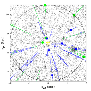
Figure 1.— Modeled OB stars (i.e. pulsar birth-sites) in the nearby Galactic plane (black dots). Detected $\gamma$-ray pulsars are also indicated (radio-selected as green circles, $\gamma$-selected as blue squares, for the distinction between these two classes, see their definitions in §2.4). Radial lines indicate the uncertainty in the distance estimates (open symbols indicate pseudo- and DM- distance estimates, filled symbols indicate parallax, kinematic, and association-based distances). The Galactic Center lies at (0, 0). The overdensity of birth sites at Galactic radii just larger than the Suns’ 8.5  kpc represents the Orion spur. Cyg OB2 is prominent toward the right side. Inner arm clusters appear toward the bottom of the plotted region.

2.2. Birth Spin Distribution and Pulsar Radio Emission

The new-born pulsar population depends critically on the distribution of spin periods at birth. This is especially important for understanding the $\gamma$-ray sample; the bulk of the radio population is sufficiently spun down to retain little memory of this adolescent phase. We describe the birth spin periods with a single parameter truncated normal distribution:

$${\rm Prob}(P)\propto e^{-\frac{(P-P_{0})^{2}}{P_{0}^{2}}}.$$ (2)

Here the spread equals the mean and we truncate at a minimum $P=10$ ms.

Faucher-Giguere & Kaspi (2006) find a characteristic birth spin period of $P_{0}=300$ ms for the radio population. However, we find that this produces very few short period, $\gamma$-detectable pulsars. Indeed, one misses producing the observed $\gamma$-ray pulsar numbers by a very large factor unless the birthrate is nearly 4 times that allowed by the observed OB stars and supernovae (i.e. more than $10\sigma$ higher than the value estimated by Li et al. 2010). Accordingly, the birth spin period distribution, for the $\gamma$-ray pulsars at least, must extend to much lower values.

It is, however, possible to reconcile this with the radio results. We find that the requirement for a large $P_{0}$ in the radio sample is a consequence of the assumed radio luminsosity law. We consider here three radio pseudo-luminosity ($L=S\,d^{2}$) laws. The first is a power law distribution that is independent of any other pulsar parameters (Lorimer et al., 2006). Next, Faucher-Giguere & Kaspi (2006) recommend a log-normal distribution whose central value scales as a power law with spin-down luminosity. Finally, we consider the broken power law distribution of Stollman (1987) for which the power law scaling of the central value stops and is flat above a cutoff (at $\dot{E}\approx 10^{34}\,{\rm erg\ s}^{-1}$). We will refer to these functions as $\rm L_{R}$ Flat, $\rm L_{R}$ Power Law, and $\rm L_{R}$ Broken Power Law, respectively.

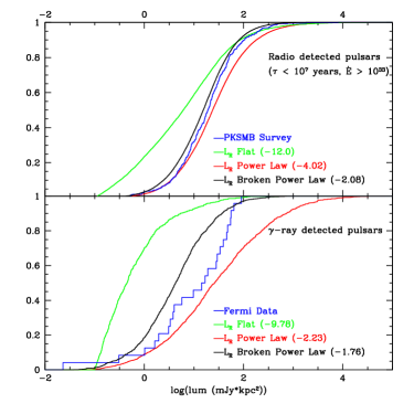
Figure 2.— Upper panel: Cumulative distribution functions of radio luminosities for a population of young radio-detected pulsars. The model CDFs show radio luminosity laws with differing spin-down dependence of the central value: Flat (green), Power Law (red) and Broken Power Law (black). These models are compared with the Parkes Multibeam sample (in blue); lower panel: same as above, but for the $\gamma$-ray-detected set, with the LAT sample in blue. The labels show the ${\rm Log_{10}}$ of the KS probability of agreement for each case.

To illustrate the effect of the initial spin and radio luminosity laws, we compare with the young pulsar populations: the LAT pulsar sample (all sky) and the high energy ($\dot{E}\ >\ 10^{33}\,{\rm erg\ s^{-1}}$) PMBS detections (within the PMBS footprint). To guage pulsar detectability we adopt a standard radio beam width

$$\rho=5.8\deg P^{-1/2}$$ (3)

(Rankin, 1993), with the assumption of a circular beam of uniform (integrated) radio flux directed along the magnetic dipole axis; we discuss briefly later the possibility that young objects have even wider radio beams from high altitude (Karastergiou & Johnston, 2007). We simulate the Galactic pulsar population as summarized above, assign a pseudo luminosity, check pulsar detectability at the modeled beam orientation and distance, compute the cumulative radio luminosity functions of the model detections (Figure 2), and compare with the observed samples. In all cases the ‘Flat’ luminosity law does not reproduced the observed luminosities, so we discard this form. The broken power law and power law distributions are quite similar for the radio sample (upper panel), but differ for the more energetic radio-detected pulsars in the $\gamma$-ray sample. We remind the reader that we have not followed the detailed selection effects of the radio surveys. However, these are unlikely to affect these conclusions. As an example, we applied a roll-off of the sensitivity with period, as in Dewey et al. (1985). Here $S_{min}=S_{0}[9w_{e}/(P-w_{e})]^{1/2}$ with the effective pulse width $w_{e}=[(0.1P)^{2}+10{\rm\,ms}]^{1/2}$ to approximate the PMBS losses at $DM\approx 200\,{\rm pc\,cm^{-3}}$. This caused only a small ($\sim 6\%$) decrease in the number of detections for the most energetic pulsars (${\rm Log}({\dot{E}})>36.5$) and negligible loss ($<$2%) from the sample as a whole. In particular, we recover the Faucher-Giguere & Kaspi (2006) result that, with the Power Law model, $P_{0}=300\,$ms provides a very good match to the PMBS radio luminosity function.

However, we see that the Fermi sample (Figure 2, lower panel) shows some discrimination between the models, especially for the high luminosity pulsars which dominate this set. The numbers of high ${\dot{E}}$ pulsars are particularly sensitive to $P_{0}$. Accordingly we have explored this sensitivity by comparing the modeled $N(\dot{E})$ of pulsars in the energetic ($\dot{E}>10^{33}\,\rm erg\,s^{-1}$) PMBS and Fermi samples as we vary $P_{0}$. Our statistic is a $\chi^{2}$ comparison of the pulsar detections in half-decade bins of $\dot{E}$. We also use the additional measurement of the Galactic core-collapse rate (and error estimate) from Li et al. (2010), fitting to the total birthrate. The results are shown in Figure 3.

As expected, this shows that with the Power Law luminosity model the radio sample prefers long initial periods, but $P_{0}=300$ ms is completely unacceptable for the $\gamma$-ray sample. This is because of the very small birthrate of energetic pulsars for this large $P_{0}$. One can, of course, imagine a $\gamma$-ray emissivisity law allowing high efficiency for detection of these very rare pulsars. The cost is that such pulsars are then extremely luminous and seen at very large distance. We find that the $\gamma$-ray pulsar sample gives such a sensitive probe of the high ${\dot{E}}$ population that changes sufficient to accomodate $P_{0}$ as large as 300 ms predict a pulsar sample in strong disagreement with the observed population (see further discussion in §4 for a specific example).

However, if we adopt the Broken Power Law radio luminosity law, we find the prefered value of $P_{0}$ for the PMBS sample decreases and that the $\chi^{2}$ at the $P_{0}\approx 50$ ms demanded by the $\gamma$-ray pulsars shows only a small increase from the minimum value. We suspect that a complete treatment of the radio survey selection effects which should decrease the detectability of short $P$ radio pulsars along the Galactic plane would further improve the agreement at small $P_{0}$.

In sum the radio and $\gamma$-ray pulsars can come from the same population if $P_{0}\approx 50$ ms and the extreme increase in radio luminosity for the shortest period pulsars is mitigated with the Broken Power Law. A second quantitative comparison of this agreement is shown in Figure 2, where we quote the model-data Kolmogorov-Smirnov comparison for the two pulsar samples for each luminosity law (here $P_{0}=50$ ms). The Broken Power Law indeed provides the best match to the detected radio luminosity function, especially for the PMBS sample. For the smaller Fermi sample the improvement is not large. We have confirmed that both this test and the $N(\dot{E})$ test are insensitive to the chosen $\gamma$-ray model (see Section 3). We thus adopt the ‘Broken’ luminosity law as the best fit to the data.

As a consistency check, applying our adopted beaming and flux law to the population, we find that the observed number of PMBS pulsars corresponds to a full Galactic pulsar birthrate of $1.43/{\rm 100\,yr^{-1}}$. This is in reasonable agreement with earlier radio population estimates and with the core-collapse estimates in §2.1 so we may turn our attention to the $\gamma$-ray-detection criterea.

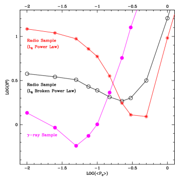
Figure 3.— Goodness-of-fit of the model to the observed data as a function of initial spin period. For each model, the pulsar population is assigned an initial spin period chosen from a normal distribution with centroid and $\sigma$ $P_{0}$. Magenta curve (filled circles) – fit to the $\gamma$-ray pulsar sample. Red curve (starred points) – the young radio pulsars, using a Power Law radio luminosity law. Black curve (open circles) – radio pulsar comparison with the Broken Power Law luminosity function.

2.3. $\gamma$-ray Emission

To complete the population synthesis we require a $\gamma$-ray pulsar flux and beaming model. Such models also depend on the pulsar’s energetics and geometry and a major goal of the data comparison is to constrain such dependence. All of the $\gamma$-ray models employed in this work utilize the same heuristic efficiency law

$$\eta=(10^{33}{\rm erg\,s^{-1}}/{\dot{E}})^{1/2},$$ (4)

with $\gamma$-ray production ceasing for objects with $\dot{E}<10^{33}\,\rm erg\,s^{-1}$. This law has theoretical motivation (Arons, 2006) and provides a reasonable match to the observed pulsar efficiencies (Abdo et al., 2010). The portion of the magnetosphere producing $\gamma$-rays and hence the fraction of the sky covered by the beam, however, differs appreciably between models.

In this paper we treat several versions of the two popular vacuum magnetosphere beaming models. The first is the standard Outer Gap (OG) model, with emission in each hemisphere produced by field lines above a single pole. In its basic form the $\gamma$-ray production is dominated by the upper boundary of a vacuum gap which is bounded by the last closed field lines and runs from the null charge surface ($\Omega\cdot B=0$) to the light cylinder $R_{LC}=cP/2\pi$. This gap has a spindown-dependent thickness approximated by

$$w=\eta=({10^{33}{\rm erg\ s}^{-1}}/{\dot{E}})^{1/2}$$ (5)

where w is the fractional distance from the last closed field lines to the magnetic axis, and the emission peaks $\sim w$ away from the closed zone. As the pulsar spins down, $w$ grows; this causes the radiating particles to approach the central field lines, the null charge crossing to move to high altitudes, and the $\gamma$-ray emission to become more tightly confined to the spin equator. To compute light curves from this simple version, we compute photon emission from particles traveling in a sheet centered on $w$, with a Gaussian cross section. As ${\dot{E}}$ decreases, we might expect pair production to become more difficult and this sheet to thicken. An extreme assumption is that emission arises from particles spanning the full thickness $w$ inward from the closed zone. Models computed for this assumption are denoted full gaps ($\rm{OG_{FG}}$). In both versions, this is essentially a ‘hollow’ cone model which tends to produce two caustic peaks, of varying separation, with a bridge between.

The other popular beaming model has emission extending from the star surface to high altitude, so that both poles are visible in both hemispheres. By truncating the emission somewhat before the light cylinder it is possible to produce models lacking the leading ‘OG’ pulse. This picture most easily produces pulses with $\sim 180^{\circ}$ phase separations and tends to have ‘Off pulse’ flux comparable to the ‘Bridge’ between the two peaks. In its original form this Two-Pole Caustic (TPC) model (Dyks & Rudak, 2003) truncates emission at the lesser of $r_{\rm{LC}}$ from the star or a distance of $0.75r_{\rm{LC}}$ from the spin axis. This basic model uses the same $w$ relation as the OG model (Equation 5).

Modifications of this geometry have been suggested as better approximations of the physical realization of such vacuum zones in the Slot Gap model (Muslimov & Harding, 2004; Grenier et al., 2010). For the first version (TPC2), the emission extends to to $0.95r_{\rm{LC}}$ and utilizes a slower, plausibly more physical, $w$ scaling:

$$w=\frac{1}{2}\,({10^{33}{\rm erg\ s}^{-1}}/{\dot{E}})^{1/6}$$ (6)

which has wide $w>0.1$ gaps even for very energetic Crab-like pulsars. Finally, we also define a full gap version of this model ($\rm{TPC2_{FG}}$), with $\gamma$-ray emission coming from the full volume between the last closed field lines and the $w$ value calculated from Equation 6.

There are also now a promising set of non-vacuum models, generated by numerical realizations of the force-free magnetosphere. One version, the ‘Separatrix Layer’ (SL) model (Bai & Spitkovsky, 2010) generates emission from field lines that start from $w\approx 0.1-0.15$ and merge in the wind zone. In this picture, $\gamma$-ray emission arises from near the light cylinder, extending several 10’s of percent past this distance. While this model has some attractive features, especially for young pulsars with robust pair production, it requires numerical realizations. We concentrate here on comparing the Fermi sample with the analytically-derived vacuum models (OG and TPC) and defer comparison with the SL model to future work.

2.4. Pulsar Samples and Detection Sensitivity

The most uniform $\gamma$-ray pulsar sample available at present is the set of 38 young objects reported in the First Fermi LAT Catalog of $\gamma$-Ray Pulsars (Abdo et al., 2010). We will refer to this as the “6 Month” sample (because that work was based on 6 months of Fermi LAT data). We also consider a larger sample of 50 young $\gamma$-ray pulsars, including all non-recycled pulsar detections announced as of July 2010. In particular, this includes the ‘blind search’ detections described in Saz Parkinson et al. (2010), as well as several individually announced discoveries. We refer to this as the “Current” sample; typically $\sim 1$ year of LAT exposure contributed toward these detections.

Fermi has two different routes to $\gamma$-ray pulsar discovery. When the signal is folded on an ephemeris, based typically on radio observation, significant pulsations can be seen to quite low levels. We term these “radio-selected” pulsars. Pulsations can also be discovered ‘blindly’, by searching directly in the GeV photons, but this method requires a somewhat higher flux for detection. We use here a threshold increase of $3\times$ for such “$\gamma$-selected” detections (Abdo et al., 2010).

A simple division of pulsars into these two classes is complicated by the discovery of several $\gamma$-ray pulsars with radio luminosities an order of magnitude or more fainter than those of the typical pulsar population (Camilo et al., 2009; Abdo et al., 2010). These sources were detected in deep, targeted integrations of young supernova remnants, unidentified $\gamma$-ray sources or detected $\gamma$-ray pulsars. Their low flux density would not be accessible in the typical sensitivity of modern large area sky surveys, 0.1 mJy at 1.4 GHz.

Since we are simulating the properties of sources detectable in large sky surveys, we wish to assign real detected pulsars to one of these classes based on their observed fluxes, not the accident of whether they had exceptionally deep radio observation. Thus “radio-selected” objects must have the survey-accessible flux density above. $\gamma$-selected objects must have the larger GeV flux required for ‘Blind search’ discovery. This results in a re-classification of several objects. There are three pulsars that had prior radio detections with 1.4 GHz flux densities below 0.1 mJy (PSR J0205+6449, 0.04 mJy; PSR J1124-5916, 0.08 mJy; and PSR J1833-1034, 0.07 mJy). For the purposes of this work, we do not consider these objects to be radio-selected $\gamma$-ray pulsars. Two of the three objects have high enough $\gamma$-ray flux levels that even without the assistance of a radio ephemeris-guided folding search, they would still have been detected as $\gamma$-selected pulsars (PSR J0205+6449 and PSR J1833-1034). Thus, these two pulsars are added to the $\gamma$-selected subset of the observed population. The third object, PSR J1124-5916, likely could not have been detected to date in blind $\gamma$-ray searches, and so is removed from the observed population. Finally, PSR J2032+4127 was found in a blind $\gamma$-ray search, but radio follow-up observations found a 1.4 GHz flux of 0.24 mJy. Thus this object “should have” been detected in radio surveys and is added to the radio-selected subset of the observed population.

With these classification amendments, the “6 Month” sample of 37 young $\gamma$-ray pulsars contains 19 radio-selected and 18 $\gamma$-selected pulsars. Similarly the “Current” sample contains 24 radio-selected and 26 $\gamma$-selected objects. These are the samples against which we will test the $\gamma$-ray emission models.

In our simulation, any $\gamma$-ray pulsar with a radio beam crossing the Earth line-of-sight with modeled flux density $>0.1\,$mJy is assumed detectable in a survey and termed radio-selected. For the $\gamma$-ray pulsars we model the phase averaged flux on the Earth line-of-sight and compare with the estimated detection threshold for each sky location plotted as a map in Abdo et al. (2010). We scale the ephemeris detection threshold with the square root of exposure time from the 6-month estimates in that paper. To be $\gamma$-selected, a modeled pulsar must exceed $3\times$ this ephemeris detection threshold, and must have a modeled radio flux density $<0.1\,$mJy at Earth.

3. $\gamma$-ray Pulse Morphology

In addition to simple detections and luminosities, the observed radio and $\gamma$-ray pulsar profiles contain a wealth of information on the pulsar emitter. We have shown in Romani & Watters (2010) how detailed analysis of the light curves, radio polarization, and other multiwavelength data can make strong model comparison statements for individual sources. Here we wish to treat the statistics of the population as a whole, so we must rely on relatively crude basic pulse properties that can be measured relatively uniformly in the discovery data. We thus characterize the pulses by $i$) the number of strong, caustic-type peaks in the $\gamma$-ray light curve $ii$) the phase differences between the radio and $\gamma$-ray peaks and $iii)$ the relative strength of $\gamma$-ray emission between (‘bridge’) and outside of (‘off’) the peaks for the common double-peaked profiles. In the following sections we quantitatively compare each of these Fermi observables with the model predictions for the pulsar population.

3.1. Peak Multiplicity

The first characteristic typically measured for a light curve is the number of peaks in the pulse profile. To compare with the data, we have taken each pulsar in our simulated Galaxy, applied the beam shape for each of the five trial $\gamma$-ray models described above, and tagged peaks with an algorithm that identifies peaks and their phases in the modeled $\gamma$-ray light curves. To increase similarity to the actual data we blocked the model light curves into 50 phase bins, before running the peak tagging algorithms. The results range from 0 peaks ($\gamma$-ray flux on the Earth line-of-sight, but no strong peak detected) to 4 or more distinct sharp peaks. Since for some models the peak morphology varies significantly with pulsar age/spin-down luminosity, we divide the sample into 4 bins of ${\dot{E}}$, logarithmically spaced.

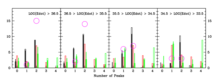
Figure 4.— Peak multiplicity histograms in four different $\dot{E}$ bins. The black bars are for the OG model, the red is for the Dyks and Rudak TPC model, and the green is for the TPC2 model. The distributtion of observed pulsars in each bin is given by the magenta circles. The thick hollow bars use a narrow Gaussian distribution of field lines around the w value specified from Equation 5 or 6, appropriately. The thin filled bars use the full gap, stretching from the last closed field lines in to the field lines specified by the appropriate w value.

The results are shown as histograms in Figure 4, with bars for each of the five models. For comparison, the measured multiplicities (always 1 or 2) for the “Current” sample are shown by the circles in each panel. It is immediately apparent that the original TPC model (central bars) produces many 3 and 4 peak light curves not seen in the data. The amendments to a slower $w$ evolution (Equation 6) and gaps extending to 0.95$R_{LC}$ (wide right bars) make this disagreement worse. Extending the emission throughout the full gap (narrow right bars) does blur out some weaker peaks, mitigating the problem. We will use this blurred version (slow $w$ evolution, fully illuminated gaps) in the remainder of the paper when we refer to ‘TPC’, as it and the original TPC model give the best match to the observed quantities. The differences in the outer gap OG predictions between the Gaussian illumination (wide left bars) and the full gap illumination (narrow left bars) is relatively minor.

We quantify the data comparison in Table 1 and Table 2. Rows 1 through 4 of Table 1 show the Poisson probability that the model is a fit to the Fermi data. Each row represents one energy bin, and the best fit model for that bin has its probability in bold. This emphasizes that the TPC2 model fairs particularly poorly without the full gap illuminated, and that for each bin the OG models provide substantially better representations of the peak multiplicity. The modeled presence of 0 peak sources (which could not, by definition, be discerned in the data) lowers the probability for all models. Also the absolute normalization is meaningful here, as these computations are run with the same model-determined pulsar birthrate (see §6). In row 5 we calculate the probability decrement of each model when compared to the best model (original OG), summed across the four energy bins. Again, in the rest of the paper we adopt the original OG and $\rm{TPC2_{FG}}$ version as the representatives of the two fiducial models.

Table 1Model Probabilities from Peak Number Comparison

	log(Poisson Probabilities)
$\dot{E}$	OG	$\rm OG_{\rm FG}$	TPC	TPC2	$\rm TPC2_{\rm FG}$
$\rm{LOG}(\dot{E})\ >\ 36.5$	-4.46	-4.66	-5.58	-8.42	-6.02
$36.5\ >\ \rm{LOG}(\dot{E})\ >\ 35.5$	-3.17	-3.59	-5.82	-11.22	-7.38
$35.5\ >\ \rm{LOG}(\dot{E})\ >\ 34.5$	-2.54	-2.75	-5.52	-8.79	-4.95
$34.5\ >\ \rm{LOG}(\dot{E})\ >\ 33.5$	-3.43	-3.19	-4.97	-7.03	-5.80
$\Sigma\Delta{\rm Log}(P)$	$\cdots$	-0.59	-8.29	-21.86	-10.55

Table 2Model Probabilities from Pulse Morphology Comparisons

	$\Delta$ - $\delta$ : 2-D KS			$\Delta$ : 1-D KS			Bridge/Off-pulse : FoM
$\dot{E}$	OG	$\rm TPC2_{\rm FG}$		OG	$\rm TPC2_{\rm FG}$		OG	$\rm TPC2_{\rm FG}$
$\rm{LOG}(\dot{E})\ >\ 36.5$	-0.96	-3.40		-2.00	-2.05		600 $\pm$ 128	462 $\pm$ 142
$36.5\ >\ \rm{LOG}(\dot{E})\ >\ 35.5$	-0.92	-3.52		-0.97	-0.72		1928 $\pm$ 268	387 $\pm$ 143
$35.5\ >\ \rm{LOG}(\dot{E})\ >\ 34.5$	-2.30	-4.52		-1.18	-0.83		552 $\pm$ 198	316 $\pm$ 159
$34.5\ >\ \rm{LOG}(\dot{E})\ >\ 33.5$	$\cdots$	$\cdots$		-0.65	-1.52		221 $\pm$ 138	143 $\pm$ 116
$\Sigma\Delta{\rm Log}(P)$	$\cdots$	-7.26		$\cdots$	-0.32		$\cdots$	-7.37

3.2. Peak Locations

A particularly powerful test of the models arises from comparing the $\gamma$-ray peak separations $\Delta$ (available for all light curves with two or more peaks, taken as the widest strong peak separation) and the lag of the first $\gamma$-ray peak from the magnetic dipole axis $\delta$. For radio-detected pulsars this axis is typically marked by the main radio pulse. The “$\Delta-\delta$” plot of these quantities is an excellent probe of the model geometry (Romani & Yadigaroglu, 1995; Watters et al., 2009). We produce such plots here in Figure 5, again with four different $\dot{E}$ bins.

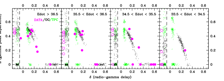
Figure 5.— 2-D plots in the $\Delta-\delta$ phase space, for the same four $\dot{E}$ bins as in Figure 4.

$\gamma$-ray pulsars that are not detected in the radio will have an undefined value of $\delta$; accordingly these objects are plotted in a band to the left, beyond the vertical dashed line at $\delta\sim-0.06$. Similarly, pulsars with only a single peak in their $\gamma$-ray pulse profiles have an undefined value of $\Delta$. We assign to these singly-peaked profiles a value $\Delta=0$ and plot in a band along the x axis. Note that in practice limited signal-to-noise in the $\gamma$-ray profiles usually prevents measurements of peak separations any closer than $\Delta\approx 0.2$, so the observed (large dots) single pulse profiles doubtless include some unresolved tight doubles, such as appear in the models particularly for small ${\dot{E}}$.

In the plots the data show a clear inverse correlation between $\delta$ and $\Delta$. This was predicted for outer magnetosphere models (Romani & Yadigaroglu, 1995) and indeed appears for the (dark) OG model points. The trend is weak or absent in the (light) TPC points. In the OG case the correlation is easily understood since both caustic peaks are generated from the magnetic pole opposite to that producing the radio emission. As the Earth line-of-sight cuts a smaller chord across this hollow cone, $\delta$ increases and $\Delta$ decreases. In contrast, the TPC model produces the first $\gamma$-ray peak from the same pole as the radio emission. The $\delta$ is nearly fixed, showing only small variation with viewing angle and age.

A less obvious difference is the OG correlation of $\Delta$ and $\dot{E}$, again weak or absent in the TPC model, which as expected shows a typical $\Delta=0.4-0.6$, with a strong concentration at $\Delta\approx 0.5$, for all spindown luminosities. In the LAT data, if we consider for each energy bin the fraction of objects with $\Delta>0.4$ we find 73% (11/15), 56% (9/16), 38% (5/13), and 17% (1/6), moving through our four energy bins from high to low.

For a quantitative measure of the goodness of fit between the data and the models, we employ a two dimensional Kolmorgorov Smirnov test (KS test) in this plane on the radio-selected samples. We can also run a standard one dimensional KS test on the $\gamma$-selected objects, for which only a $\Delta$ value exists. The probabilities from these tests are displayed in Table 2. With only a single detection, the 2-D KS test is unavailable for the lowest $\dot{E}$ bin. The bottom row of Table 2 (as for Table 1) gives the summed probability decrement compared to the best (OG) model; although the OG model itself is not adequate (Prob $\sim 10^{-4}$), probabilities for the TPC models are factors of $\geq 10^{7}$ lower. Statistically, the OG model is strongly preferred.

Single peaked (x-axis) $\gamma$-ray light curves deserve some additional discussion. As noted above, objects may appear here when the data do not resolve a double. Such objects in the OG picture are expected to appear at $\delta\approx 0.3-0.4$. In the OG model, a peak may also be single if the first $\gamma$-ray peak is missing. Since this caustic forms at high altitudes, it is rather sensitive to field line distortion from sweep back and to aberration effects, especially for moderate to large $\dot{E}$. In the vacuum models, we find that this caustic (and peak) are often missing for energetic pulsars when the observer line-of-sight lies well away from the spin equator. Near the spin equator the caustics are unaffected, so that large $\Delta$ appear, but smaller $\Delta<0.3$ are missing for energetic pulsars. As a result $\delta$ is large ($\sim 0.5-0.6$) since it now measures the distance to what is normally the second pulse. This effect may be seen in the models and data of the left panels of Figure 5. However, it should be noted that the sensitivity of the first peak caustic to field line perturbations makes the extent of this effect difficult to predict. For example Romani & Watters (2010) found that open zone currents can reduce or eliminate such first peak ‘blowout’, so realistic models containing plasma may affect the prevalence of large $\delta$.

Finally, it should be noted that if small altitude emission occurs, then the trailing side of the radio-producing pole may form a caustic (this is the first peak in the TPC picture). As seen by the heavy concentration of TPC model dots in Figure 5, this results in $\delta\approx 0.1$ . The Fermi LAT may have in fact uncovered one such object: PSR B0656+14, which appears near $\delta=0.2$ in the third panel, has a single pulse, a peculiar soft spectrum and an apparent luminosity $\sim 30\times$ smaller than seen from similar $\dot{E}$ pulsars. Polarization modeling suggests that it has a very small $\alpha$ and $\zeta$, so that its outer magnetosphere beam should miss the Earth. In this interpretation we only see the fainter low altitude emission because of this pulsar’s very low distance.

Thus $\delta$ provides a useful way of sorting pulsar properties, even when only a single $\gamma$-ray peak is available. Improved S/N, polarization studies and, above all more physical magnetosphere modeling, should help us calibrate this diagnostic.

3.3. Bridge and Off-pulse Emission

The most common $\gamma$-ray profiles contain two peaks, and for these profiles we can introduce a third measure of pulse shape that can be applied to the bulk sample: the strength of the intra-peak (‘bridge’) and inter-peak (‘off-pulse’) emission. To estimate these flux levels we divide the double peaked profiles into 4 phase windows. Two intervals of $\Delta\phi=0.14$ (7 bins in a 50 bin light curve) are centered on the main peaks and the two remaining phase intervals (totaling 0.72 of pulse phase) are assigned to the ‘bridge’ and ‘off-pulse’. We next measure the mean flux in each of these phase windows. We then report the bridge fraction as $\langle$bridge$\rangle$/$\langle$(bridge+peaks)$\rangle$ and the off-pulse fraction as $\langle$off-pulse$\rangle$/$\langle$(bridge+peaks)$\rangle$. This easily defined measure generally corresponds well to a visual definition of bridge and off pulse intervals, although it does not always isolate well the absolute pulse minimum. We plot these two fluxes for the model light curves, in the usual four panels of spin-down luminosity, in Figure 6.

Figure 6.— 2-D plots in the bridge emission $vs.$ off-pulse emission phase space, for the same four $\dot{E}$ bins as in Figure 4. Estimated measurements for observed double-peaked pulsars are plotted, assuming a 10% uncertainty in the background levels reported in the discovery papers. Only objects with high ($>2\sigma$) significance have dots associated with the plotted error bars.

Clearly these quantities provide good model discrimination. Models radiating only in the outer magnetosphere (e.g. OG) have little off-pulse flux, especially for older pulsars, while models radiating at all altitudes have comparable bridge and off-pulse emission. In particular, the TPC picture produces essentially no light curves with off-pulse fluxes less than 40% of the pulse phase emission.

Unfortunately, unlike the peak number and separation, such fluxes are not provided in Abdo et al. (2010), Saz Parkinson et al. (2010) and the other discovery papers. One difficulty in making such measurements is the identification of the true background level. In practice it can be very difficult to distinguish unpulsed “DC” magnetospheric emission from the contribution of an unresolved background in close proximity to the pulsar, such as expected from a surrounding pulsar wind nebula. Detailed study of source extension and spectrum at pulse minimum can help distinguish these cases, but this goes beyond the pulsar catalog data.

Nevertheless, the published light curves do plot an estimated background flux level. Accordingly we entered these light curves, defined the peak and intervening intervals exactly as above and measure the bridge and off-pulse flux levels. We assume a systematic 10% uncertainty in the reported background level, and then propagate this and the Poisson uncertainties in the bridge-, off-, and average-pulse fluxes to produce the two flux ratios and errors defined above. In a few cases the background level defined in Abdo et al. (2010) were above the measured pulse minimum. In those cases, we reassigned the background flux to this level (and by definition the off-pulse flux was then 0). In a number of cases, the very large background pedestal prevented accurate measurements. While we show error bars for all estimates of double pulse pulsars in Figure 6, we mark with large dots only those measurements which had either a 2$\sigma$ significance measure of both flux ratios, or a ratio less than 0.1 at 2$\sigma$ significance.

Bridge emission varies from $\sim 0.3\times$ to $>1\times$ the average pulse flux at all spindown luminosities, although a few high ${\dot{E}}$ objects seem to have virtually no emission away from the peaks. In contrast, the majority of the objects have $0.3\times$ or less of the pulse emission in the off-peak window. Most of the best measured pulsars show very small values. Values of $\sim 0.1-0.3\times$ appear for a number of the most energetic pulsars, but these measurements are of poor statistical significance. In any case such objects are most likely to show unpulsed contamination from associated PWNe, supernova remnants and other diffuse, but unresolved emission. Thus overall, the general distribution of measured values matches better to the OG predictions, as shown in Table 2.

Nevertheless, several objects are distinctly inconsistent with emission from only high altitudes. In particular PSR J2021+4026 (panel 3) and PSR J1836+5925 (panel 4), show very strong off pulse emission, which is spectrally consistent with magnetospheric emission (hard with a few GeV exponential cut-off). These unusual objects lie squarely within the TPC model zone. Interestingly both are quite low ${\dot{E}}$, and both have $\Delta$ very close to 0.5, consistent with a low altitude, two-pole interpretation. Also, the very energetic PSR J1420-6048 (panel 1) shows strong off pulse emission. Here, with $\Delta=0.26$ a low altitude interpretation is not natural. However, unlike the other two cases, the very large and poorly determined background (from the bright PWN emission in the surrounding ‘Kookaburra’ complex) may exceed the catalog background flux level. However it is clear that, at least in a few cases, an emission component other than the outer magnetosphere of the OG model contributes substantially to the pulse profile. An excellent candidate is low altitude emission, such as posited in the TPC model. An alternative is a current-induced shift of the outer gap start below $r_{NC}$ (Hirotani, 2006). It will be particularly interesting to discover the physical effect that causes such emission to be significant for a few pulsars, but negligible for most.

4. $\gamma$-ray Evolution with $\dot{E}$

As illustrated in the four-panel Figures 4-6, the pulse profile properties evolve as the pulsar ages and ${\dot{E}}$ decreases. In addition there is of course strong evolution in the pulsar luminosity. Together, these trends strongly affect the pulsar detectability in the two detections classes ($\gamma$-selected and radio-selected) as a function of spindown flux. We explore these population effects in this section.

In Figure 7 we plot histograms of detection numbers versus spin-down luminosity, for both the radio-selected (top panel) and $\gamma$-selected (middle panel) subsets. The blue histogram shows the simulated OG model detections, while the black data points show the Fermi results, with statistical error bars. In the bottom panel we plot the “Geminga Fraction,” or fraction of the total number of detected pulsars which are $\gamma$-selected.

The OG model gives a reasonably good fit to the Fermi data, with $\chi^{2}$ Gehrels fits of 0.587 per degree of freedom for the radio-selected population, 0.251 per degree of freedom for the $\gamma$-selected population, and 0.054 per degree of freedom for the Geminga Fraction. Ravi et al. (2010) have noted that in the 6 month sample the most energetic $\gamma$-ray-detected pulsars are all radio-detected as well. They argue that this implies a large radio beam, roughly co-located with the $\gamma$-ray emission region for these most energetic (${\dot{E}}>6\times 10^{36}{\rm erg\,s^{-1}}$) pulsars. This may be caused by high altitude emission as posited in Karastergiou & Johnston (2007). Our model, without high altitude radio beams, predicts 7-8 such very high $\dot{E}$ pulsars in the 6 month sample, of which 2-3 should be undetectable in the radio (i.e. our line of sight is outside of the radio beam). The actual LAT sample had 7 such pulsars, all of which were detected in the radio. We have simulated high-altitude radio emission, confirming that it prevents the $\gamma$-ray only detections at the highest $\dot{E}$. However, we conclude that the present sample is too small to use these numbers to probe the detailed behavior of such objects with high statistical significance; for the moment the case for high altitude radio emission still largely relies on the radio pulse properties.

There does exist one moderately significant defect in the histogram for low $\dot{E}$ radio-selected pulsars; the model predicts too many such detections. This is reflected as well in the Geminga Fraction, where the data demand a larger value for the Geminga Fraction at low energies. Such an increase is not seen in the model, due to the excess of radio-selected detections. For now we note the discrepancy, but refer to Section 5 for discussion of a possible solution.

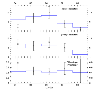
Figure 7.— Histograms of detection numbers versus $\dot{E}$. The model overproduces radio-selected $\gamma$-ray pulsars at low $\dot{E}$.

Spin-down luminosity should, through the $\gamma$-ray efficiency, be correlated with the typical distance of the detected pulsars. Unfortunately, as we have seen, distances estimates (and hence inferred luminosities) are very poor for many of these objects. However, Galactic latitude correlates inversely with distance and is a directly observable property. Accordingly, in Figure 8 we show the ${\dot{E}}-b$ planes for the radio-selected and $\gamma$-selected subsets. The colored points show the locations of Fermi pulsars and the contours show the density of the OG model detections.

The modeling predicts a dramatic increase in the latitude spread of the lowest ${\dot{E}}$, (lowest $L_{\gamma}$, nearest) objects. The $\gamma$-selected set actually shows this trend quite well. In contrast, the radio-selected pulsars show a distinct lack of the nearby, lower luminosity higher latitude objects predicted by the models at log$(\dot{E})<34.5$. This is directly connected to the simple lack of low $\dot{E}$ radio-selected objects noted above. Also in the radio panel, one notices the very high $\dot{E}$ Crab pulsar – which is surprisingly close for such an energetic pulsar and notoriously far from the plane. This distance off the plane is likely a product of an unusually long-lived low mass runaway progenitor from the Gem OB1 or Aur OB1 associations.

The model agreement is tested with a two dimensional KS test. For the $\gamma$-selected sample one gets a KS probability of 3.9%, quite acceptable for this population model. For the radio-selected sample the KS probability is however only 0.5%, which is not a good agreement. The discrepancy is largely driven by the missing ${\dot{E}}<10^{35}\ \rm{erg\ s^{-1}}$ pulsars; if this region is excluded the KS probability rises to 2.6%, which is not excludable.

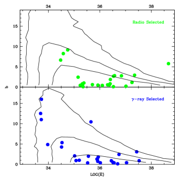
Figure 8.— 2-D plot of detections in the $\dot{E}$-galactic latitude plane. Note the overproduction of model detections at low $\dot{E}$ in the radio-selected sample.

With the caveat about observational uncertainties noted above we can also compare with the data in the $\dot{E}$-$d$ plane (Figure 9). Here we expect small $d$ at low $\dot{E}$. In an attempt to illustrate the distance uncertainties, we use different symbols to plot objects with distance estimates from various sources (drawn from the discussion in the discovery catalogs). For example, radio detected pulsars have Dispersion Measure (DM) distance estimates. These are shown as open circles. While generally held to be accurate to $\sim 30$% for the bulk of the pulsar population, these estimates evidently have much larger fractional errors for the energetic LAT pulsars near the plane and, in a number of cases, are clearly substantial overestimates. In some cases we have other distance estimators ranging in reliability from astrometric parallax (very high) through HI absorption kinematics to spatial associations (low). These objects are plotted with filled dots. Note that in the upper panel of Figure 9 these distances average lower than the DM values for all ranges of $\dot{E}$.

Finally, for a number of $\gamma$-selected pulsars we have no estimate of distance other than assuming a $\gamma$-ray efficiency (Equation 4) and isotropic emission and using the observed $\gamma$-ray flux to estimate $d$. Such estimates are referred to as “pseudo-distances” (Saz Parkinson et al., 2010), and while they provide helpful consistency checks, their use is, to some degree, circular if employed to test a model. They are plotted as crosses.

Examining the 2-D KS test probabilities, we find that the radio-selected sample returns a probability of 0.7%. As for the $\dot{E}-b$ set, this is moderately excludable. Again, a re-test using only objects above $10^{35}\ \rm{erg\ s^{-1}}$ delivers a higher probability of 2.3%. The probability for the $\gamma$-selected sample is 19.9%. This large value is certainly partly due to the use of the pseudo-distances. However, even after removing these objects, we find a probability of 10.4%, suggesting that the model is a quite good representation of the data.

Thus our heuristic $\gamma$-ray luminosity law (Equation 4) and our Broken Power Law radio-luminosity law provide a good match to the data. Other models provide a much poorer match. For example, a simple linear $\gamma$-ray luminosity law $L_{\gamma}=1/3{\dot{E}}$  together with the straight Power Law radio luminosity law and large birth period $\langle P_{0}\rangle=300$ ms recommended by Faucher-Giguere & Kaspi (2006) can produce a reasonable number of $\gamma$-detectable pulsars for a Li et al. (2010) birthrate. However the predicted distances are $2\times\;-\;4\times$ those observed and 2-D KS comparisons in the ${\dot{E}}-b$ and ${\dot{E}}-d$ planes produce unacceptably low probabilities for the radio-selected $\gamma$-ray sample ($9\times 10^{-4}$ and $7\times 10^{-4}$, respectively).

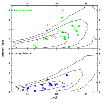
Figure 9.— 2-D plot of detections in the $\dot{E}$-distance plane. The overproduction of model detections at low $\dot{E}$ in the radio-selected sample is still evident.

5. Possible Amendments to the $\gamma$-ray Model

We have shown how to quantitatively compare the observed properties of the LAT pulsar survey to predictions of population models. While the agreement is generally quite good, in particular for the models dominated by outer magnetosphere radiation, some discrepancies are already seen. Our ability to study such discrepancies will certainly improve as the size of the LAT sample and the quality of the individual light curve measurements increase. Thus we wish to discuss sensitivities of the observed data sample to details of the beaming model and amendments to the modeling that may further improve the fidelity of the synthesized population.

As an example, we should consider how beaming and luminosity evolve at low $\dot{E}$ as $w$ and the pulsar efficiency approach a maximum and the gap saturates and shuts off. In particular, for the OG model, since emission starts above the null charge surface, large $w$ drives this start toward the light cylinder and produces a decreasing $\gamma$-ray beam solid angle.

If one follows the simple efficiency law (Equation 4) into such a regime then phase average pulse intensity for the few observers seeing all of $\eta\dot{E}$ in this very small angle would become very large just before the beam shuts off. In principle, this allows a small number of $\dot{E}<10^{34}\,\rm erg\,s^{-1}$ pulsars to be seen at very large distances. The more physical alternative, adopted here, is to link $\eta\dot{E}$ to the ‘surface brightness’, the thickness-integrated emissivity per unit area of the gap volume. For all ${\dot{E}}$ producing modest $w$ this means $L_{\gamma}\propto w$ or $\propto w^{3}$, as usual. However as $w$ approaches unity and the active gap area contracts laterally, the total sky-integrated luminosity smoothly goes to $0$ at gap saturation, although the surface brightness continues to grow. To illustrate the sensitivity of the data-population comparison to such effects we illustrate (Figure 10) the different prediction of these two cases. The left panels reproduce the low ${\dot{E}}$ end of Figure 9, while the right panels show the increased distance reach – from $\lesssim 1\,$kpc to $\gtrsim 3\,$kpc – if all the power is forced into the decreasing beam. As it happens the effect is largely concentrated in the $\gamma$-selected pulsars, since to produce emission from such large $w$, $\alpha$ must be moderate to small (i.e. $\alpha\lesssim 50^{\circ}$), but the viewing angle $\zeta$ must be very near the equator (i.e. $\zeta\gtrsim 85^{\circ}$). For such objects the radio beam misses Earth. This and even more subtle evolution effects will become increasingly subject to test as the LAT sample grows.

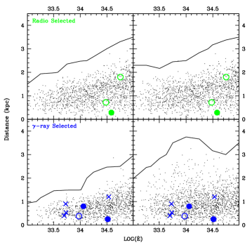
Figure 10.— Figure showing the effects of forcing the model to pump $\eta\dot{E}$ power into the $\gamma$-ray emission region, regardless of how small that region becomes. Note that we have zoomed in here on the region of interest, $\dot{E}<10^{35}\rm{ergs^{-1}}$.

We have already alluded to another deficiency in our modeling of the low ${\dot{E}}$ population; the substantial over-prediction of radio-selected objects. In fact, there is an evolutionary process that can be amended to our model to produce exactly this effect: magnetic alignment. Recent work has suggested that a secular decrease in $\alpha$ may occur on timescales as short as 1 Myr (Young et al., 2010). Given the high sensitivity of the $\gamma$-ray beaming to $\alpha$ for some models, even partial alignment can have a large effect on our young pulsar population.

We describe here qualitatively the main effects, deferring detailed population predictions to a study including the alignment kinematics. As $\alpha$ decreases with age, there are two main effects on the pulse observables in the OG model: a decrease in the average $\Delta$ and a decrease in the number of total detections, with an especially strong elimination of radio-selected objects. These should show up principally at the largest ages (i.e. lowest $\dot{E}$ values) of the $\gamma$-ray pulsar population.

The first OG effect, a decrease in typical $\Delta$ values, results from the fact that the highest $\Delta$ values are always produced by large $\alpha$ models. Eliminating such models would have the effect of shifting the clump of $\Delta\sim 0.4$, $\delta\sim 0.15$ models in Figure 5 panel 4 to $\Delta\sim 0.2$, $\delta\sim 0.25$. Of course we need substantially more low ${\dot{E}}$ pulsar detections before any such evolution can be tested.

The second OG alignment effect is a reduction in $\gamma$-ray detections at low $\dot{E}$. In outer gap geometries, the approach of the null charge crossing to the magnetic axis and light cylinder occurs at higher $\dot{E}$ for aligned pulsars. Thus gaps saturate and shut off at younger ages (i.e. higher $\dot{E}$ values) the more aligned a pulsar is. This has pulse shape effects, but most importantly causes more rapid depletion of the smaller $\alpha$ pulsars. In fact, the process preferentially eliminates radio-selected $\gamma$-ray pulsars. We illustrate this in Figure 11. The main field in that figure shows the $\alpha-\zeta$ plane, populated with detected $\gamma$-ray pulsars. $\gamma$-selected pulsars are shown with open black circles, while radio-selected pulsars are shown with filled red circles. The radio-selected objects must have small $|\beta|=|\zeta-\alpha|$.

As alignment proceeds, we expect that the largest $\alpha$ values will migrate to lower $\alpha$. Note that as angles from $80^{\circ}-60^{\circ}$ are depleted (hatched zone), many more radio-selected objects than $\gamma$-selected objects are lost. Additionally, many radio-selected objects actually become $\gamma$-selected objects, while the converse is much more rarely the case. This is illustrated in the figure inset, showing the effects of an increasingly large shift in alpha values. The number of radio-selected detections drops much faster than the $\gamma$-selected detections (which in fact increases at some points, for the reason mentioned above) and the Geminga fraction grows toward unity.

Since the principal alignment effects amend discrepancies seen in the data comparison, a more complete study seems warranted. In particular, the high sensitivity of outer magnetosphere models to $\alpha$ can make the effects of even subtle alignment more easily detected than in the radio data, which is largely controlled by $\beta$. Note that lower altitude models, such as TPC, are much less affected by alignment. In practice we might expect some spread in the alignment rates with a few objects persisting at large $\alpha$ to relatively late times so a detailed kinematic study may be required.

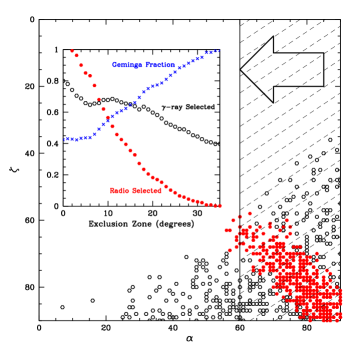
Figure 11.— Figure showing the effects of magnetic alignment on the detection fractions of older ($\dot{E}\leq 2.5\times 10^{34}\,{\rm erg\,s^{-1}}$) $\gamma$-ray pulsars.

6. Discussion, Conclusions, & Predictions

We have simulated a model Milky Way Galaxy filled with young pulsars, and by comparing the distributions of various observables we have been able to constrain properties of the true population and evaluate the relative fidelity of several $\gamma$-ray pulsar models. To start, we found that a radio luminosity distribution scaling with ${\dot{E}}$ can provide a good fit to the observations, but only if the scaling relation is broken and plateaus at the very highest luminosities. We also find that the $\gamma$-selected sample has so many pulsars with large spin-down luminosity that a short birth period distribution ($\langle P_{0}\rangle\approx 50\,$ms) is required. These parameters also provide a good description of the young radio pulsar population.

In comparing with several $\gamma$-ray emission models, all based on the vacuum dipole field structure, we find that Outer Gap (OG) models perform the best in almost all circumstances. Thus, for the population as a whole there is a very statistically significant (formally $\geq 10^{7}\times$) preference for the OG model – i.e a model dominated by radiation above the null charge surface. However,, there are a handful of individual objects that do not fit easily into the predicted OG population. Such objects may well have significant lower altitude emission, as posited by Slot Gap (TPC-type) models. Discerning the physical parameters which select when such emission is present will be particularly interesting. It should also be remembered that while these vacuum calculations give a clear preference for OG geometries over TPC geometries, they are themselves not perfect fits and do not represent complete physical models. This is evident since even the OG model does not produce $\chi^{2}$/DoF=1. This is not surprising since any real magnetosphere must include some currents and plasma affects will certainly perturb the vacuum conclusions. Thus it will be of interest to extend this population model/data comparison to the other extremum, the fully force free plasma-dominated SL models (Bai & Spitkovsky, 2010).

We conclude this discussion by making future predictions of the pulsar birthrate, detectable numbers and background contribution for the preferred OG model. The 6 Month sample from Fermi contains 37 $\gamma$-ray pulsars, with a Geminga Fraction of 49%. At the 6 Month sensitivity level, the OG model produces 2194 $\gamma$-ray detections (normalized to one pulsar birth per year) with a Geminga Fraction of 46%. Thus the observed pulsar count directly gives the pulsar birthrate: $2194/37\approx 59$ years per pulsar birth, or $1.69\pm 0.24({\rm stat})\rm\ pulsars\ century^{-1}$. This is in excellent agreement with the core collapse rate (Diehl, 2006) and OB star birthrate (Reed, 2005) measurements quoted in Section 2.1. It is also only $1.2\sigma$ lower than the SN rate computed by Li et al. (2010), which has the smallest formal error bars.

It is interesting to compare this birthrate estimate to the independent O-B2 star birthrate estimate made in this work, based on the local massive star density ($2.4\rm\ OB\ century^{-1}$). The first thing to note is that our $\gamma$-ray pulsar birthrate is a large fraction of these progenitor rates. For example, at 71% of the O-B2 star rate, a large fraction of these stars must produce $\gamma$-ray pulsars. Indeed we check if culling the lowest mass class (B2, $\sim 9M_{\odot}$) is acceptable. With this cut the local massive star birthrate drops from $40\rm\ OB\ kpc^{2}\ Myr^{-1}$ to $21.5\rm\ OB\ kpc^{2}\ Myr^{-1}$, which corresponds to a Galactic rate of $1.3\rm\ OB\ century^{-1}$. This is only 75% of the rate needed to produce our inferred $\gamma$-ray pulsar population. This is also 2.1$\sigma$ lower than the Li et al. (2010) Galactic supernova rate. Thus we conclude that B2 stars should produce SNe and contribute to the young pulsar population.

Perhaps even more interesting is the direct comparison between our pulsar birthrate and the core collapse rate. The observed $\gamma$-ray pulsars contribute $>75\%$ of the (relatively high) inferred SN rate in this study. Thus we conclude that the $\gamma$-ray pulsar sample must be an excellent census of the local core collapse products. These rates imply that no more than 25% of the core collapses can produce slow $P_{0}$ injected pulsars, RRATS, Central Compact Sources in Supernova Remnants, magnetars and other exotica. Similar conclusions have already been reached by Keane & Kramer (2008) using the radio surveys. Thus our new population estimate, derived from the Fermi sample and sensitive to $\gamma$-ray rather than radio beaming effects, supports the picture that energetic radio pulsars dominate the neutron star birthrate, and that more exotic objects cannot contribute a dominant fraction of the neutron star population unless they represent a later phase in the evolution of energetic, $\gamma$-ray producing pulsars.

In outer magnetosphere models there are, of course, some pulsars whose bright $\gamma$-ray beam misses the Earth while the radio beam does not. These objects can be detected in the radio but will be absent in the $\gamma$ rays, despite the fact that they are $\gamma$-ray active. This especially occurs for geometries with small $\alpha$ and small $\zeta$ (see Figure 11 where radio-only pulsars continue to the upper left); for a few objects, known angles place them in this region, e.g PSR J1930+1852 (Ng & Romani, 2008; Abdo et al., 2010). Of course, fainter low altitude emission aligned with the radio could still be visible; PSR J0659+1414 could be such a case. Our population estimates suggest that there should be a modest number of objects in this radio loud, $\gamma$-ray missed category. At the sensitivity of the 1 year sample we would expect $\sim 10$ radio-detected, $\gamma$-ray undetected pulsars with ${\dot{E}}>10^{33.5}$ and ${\dot{E}}^{1/2}/d^{2}$ as large as that of the faintest detected $\gamma$-ray pulsars; again, these are objects not seen in the $\gamma$-rays simply due to beaming effects. Most of these have ${\dot{E}}<10^{35}\,{\rm erg\,s^{-1}}$. As the $\gamma$-ray sensitivity grows, the fraction of such objects decreases. However there are also pulsars whose radio and $\gamma$-ray beams both miss the Earth. At the 1-year sensitivity nearly half of the pulsars with ${\dot{E}}^{1/2}/d^{2}$ above that of the faintest detections are such ’Isolated Neutron Stars’ (INS). Such radio-only pulsars and INS are implicitly included in the birthrate estimates above.

Given the successes of the OG model at matching the observed population, it is natural to ask what this scenario predicts as we acquire additional observations. For the birthrate above, we can lower the $\gamma$-ray threshold and make predictions of the number of detections as a function of Fermi observation time. Our “Current” Fermi sample is based on approximately one full year of data; extrapolating from the 6-month normalization, we find that the model predicts 23 $\gamma$-selected pulsars and 26 radio-selected pulsars. The actual observed sample contains 24 $\gamma$-selected pulsars and 26 radio-selected pulsars, an excellent match to the observations. Similarly after five years exposure the model predicts 49 and 44 detections and after ten years 65 and 55, $\gamma$-selected and radio-selected detections, respectively. With the improved 10-year $\gamma$-ray sensitivity, the number of radio-detected, $\gamma$-ray undetected pulsars grows at a similar rate; we expect $\sim 27$ such objects with $\dot{E}^{1/2}/d^{2}$ large enough that we would expect detection. The number of INS whose $\gamma$-ray beam would be detectable, if directed at Earth, grows to $\sim 150$ objects, still about 1/2 of the total population. Most are again low ${\dot{E}}$ pulsars whose relatively narrow radio and $\gamma$-ray beams only sweep a small fraction of the sky.

Note that we can hope that the actual $\gamma$-ray pulsar numbers will be larger by a modest fraction as analysis and search techniques improve and as deep radio observations lower the effective survey threshold. Note also that these numbers do not include the very substantial population of recycled pulsars now being detected; the equivalent analysis of this population will be prosecuted in future work.

The trend towards higher Geminga Fraction above in these future predictions is due to two effects. First, as Fermi probes larger distance scales our radio pulsar sample will not be as complete. In practice, as just noted, deeper radio searches will mitigate this trend. Of course, we still expect a substantial number of very low flux density sources will still remain non-detected, since the present very deep radio searches on many LAT sources indicates that these are a substantial part of the Geminga population. The second effect increasing the Geminga Fraction is a change in the $\dot{E}$ distribution of the detected pulsars. The five and ten year model samples have a higher proportion of mid to low luminosity objects ($\dot{E}\lesssim 10^{35}\,{\rm erg\ s}^{-1}$), and thus proportionately fewer energetic pulsars. With longer periods at lower $\dot{E}$ come narrower radio beams and fewer detections. If alignment, as discussed above, is included in the models this contribution to the Geminga fraction will be even larger.

The final number to report is the $\gamma$-ray background supplied by unresolved pulsars. To compute this we simply sum up the emission from sources not individually detected (at a given LAT exposure time). To estimate the spectral content of this contribution, we assign each modeled pulsar a power-law spectral index $\Gamma$ and exponential cut-off energy $E_{c}$. The assigned value is inferred from the $\Gamma({\dot{E}})$ and $E_{c}(B_{LC})$ trends visible in Figures 7 and 8 of Abdo et al. (2010) and approximated here by

$$\rm{E_{c}}=[-0.45+0.71\,\rm{log(B_{LC})}]\,{\rm GeV}$$

$$\Gamma=-4.10+0.156\,\rm{log(\dot{E})}.$$ (7)

These model spectra can be used to sum up the effective young pulsar background spectrum. In practice we compute 0.1-1 GeV and 1-10 GeV sky maps of this emission to look for any interesting spatial distribution. Some evidence of cluster structure is seen in these maps, but in any event the contribution to the total Galactic background is small.

At the 6 month sensitivity limit we find that pulsars supply $4.4\times 10^{-9}\,\rm erg\ cm^{-2}\ s^{-1}$ (1.8%) of the total background flux in the 0.1-1 GeV band and $3.6\times 10^{-9}\,\rm erg\ cm^{-2}\ s^{-1}$ (2.8%) of the flux in the 1-10 GeV band (integrated over the full sky and compared against the Fermi Collaboration’s publicly available background skymap, gll_iem_v02). Of course, as time progresses and more pulsars are individually detected, the total unresolved flux from background pulsars goes down. After 10 years of observation, approximately half of the total flux unresolved at 6 months will have been detected as individual sources. We would then find that pulsars contribute only 1.0% and 1.5% of the 0.1-1 Gev and 1-10 GeV background bands, respectively. We remind the reader that this does not include the contribution of recycled pulsars. As noted, some studies (Faucher-Giguere & Loeb, 2010) estimate that this may be quite substantial at intermediate latitude. A treatment with improved luminosity, beaming and evolutionary effects, as presented here for the young pulsar population, seems very desirable.

References

- Abdo et al. (2010) Abdo, A.A. et al 2010, ApJ, 187, 460.
- Abdo et al. (2010) Abdo, A.A. et al 2010, ApJ, 711, 64.
- Arons (2006) Arons, J. 2006, 26th IAU, Parugue, JD02 #39, 2
- Bai & Spitkovsky (2010) Bai, Xue-Ning & Spitkosky, Anatoly. 2010, ApJ, 715, 1282.
- Camilo et al. (2009) Camilo, F. et al. 2009, ApJ, 705, 1.
- Cordes & Lazio (2002) Cordes, J.M. & Lazio, T.J.W. 2002, arXiv, astro-ph, 0207156.
- Dewey et al. (1985) Dewey, R. et al. 1985, ApJ, 294, L25.
- Diehl (2006) Diehl, Roland et al. 2006, Nature, 439, 45.
- Dray (2006) Dray, L.M. et al. 2006, Ap&SS, 304, 279.
- Dyks & Rudak (2003) Dyks, J. & Rudak, B. 2003, ApJ, 598, 1201.