Phase diagram of the ABC model with nonconserving processes

Abstract

The three species ABC model of driven particles on a ring is generalized to include vacancies and particle-nonconserving processes. The model exhibits phase separation at high densities. For equal average densities of the three species, it is shown that although the dynamics is local, it obeys detailed balance with respect to a Hamiltonian with long-range interactions, yielding a nonadditive free energy. The phase diagrams of the conserving and nonconserving models, corresponding to the canonical and grand-canonical ensembles, respectively, are calculated in the thermodynamic limit. Both models exhibit a transition from a homogeneous to a phase-separated state, although the phase diagrams are shown to differ from each other. This conforms with the expected inequivalence of ensembles in equilibrium systems with long-range interactions. These results are based on a stability analysis of the homogeneous phase and exact solution of the hydrodynamic equations of the models. They are supported by Monte-Carlo simulations. This study may serve as a useful starting point for analyzing the phase diagram for unequal densities, where detailed balance is not satisfied and thus a Hamiltonian cannot be defined.

Draft date : March 1, 2024

Keywords: Driven diffusive systems (Theory), Classical phase transitions (Theory), Stochastic particle dynamics (Theory)

1 Introduction

Systems driven out of equilibrium by an external field, such as a temperature or a pressure gradient or by an electric field, have been a subject of extensive studies in recent years (see [1, 2] for reviews of this topic). Often, such systems reach a current carrying steady state where detailed balance is not satisfied. The nature of the steady state typically depends on the details of the microscopic dynamics. This is in contrast to systems in thermal equilibrium where the equilibrium distribution is determined by the Hamiltonian, and is independent of the microscopic dynamics. Thus, for instance, in the Ising model, the same equilibrium state is reached in the thermodynamic limit irrespective of whether the dynamics is magnetization conserving (Kawasaki dynamics) or magnetization nonconserving (Glauber dynamics).

Insight into the properties of nonequilibrium steady states has been obtained by detailed studies of simple models of particles on a lattice, where the particles are driven by either boundary terms or in the bulk. The behavior of these driven systems has been shown to be nontrivial, as they exhibit phenomena which do not occur in equilibrium. In particular, nonequilibrium steady states of driven systems have been found to exhibit long-range correlations, even for systems with strictly local dynamics [3, 4, 5, 6, 7, 8]. While attempting to understand the nature of these long-range correlations, several studies revealed similarities between some properties of driven nonequilibrium systems and equilibrium systems with long-range interactions. One example is the presence of phase transitions in one-dimensional driven models [9, 10, 11], which are known to exist also in equilibrium systems with long-range interactions. An interesting question, which is addressed in the present paper, is to what extent can studies of equilibrium long-range systems provide some understanding of properties of driven nonequilibrium systems.

Equilibrium systems with long-range interactions are those where the two body potential decays at large distance, $r$, as $1/r^{d+\sigma}$, with $-d\leq\sigma\leq 0$ in $d$ dimensions. In this case the total energy of a system of homogeneously distributed particles scales as $V^{1-\sigma/d}$ with its volume $V$. Therefore, if $-d\leq\sigma\leq 0$, the energy scales super-linearly with $V$, and the system is nonadditive. As a result of the nonadditivity the various statistical mechanical ensembles may become inequivalent [12, 13, 14, 15, 16, 17, 18, 19, 20]. For example, it is well known that the specific heat of long-range interacting systems can be negative in the microcanonical ensemble. On the other hand within the canonical ensemble the specific heat is proportional to the energy fluctuations, $C_{V}\propto\langle E^{2}\rangle-\langle E\rangle^{2}$, and always positive. Similar effects can be found when comparing the canonical and grand-canonical ensembles of long-range interacting systems [21]. It has been suggested that differences between ensembles in these systems are usually manifested in the vicinity of first order phase transitions [19, 22, 23, 24]. For recent reviews of systems with long-range interactions see e.g. [25, 26, 27, 28, 29]. Finding similar features in nonequilibrium driven systems would thus provide a further link between the two classes of models.

A particularly interesting model within which the interplay between drive and long-range interaction may be conveniently analyzed is the ABC model. This is a one-dimensional driven model on a ring where three species of hard-core particles evolve under particle conserving local stochastic dynamics. The model has been introduced by Evans et al. [30, 31] who observed that although the dynamics of the model is local, it exhibits long-range order characterized by phase separation of the three species. It has been found that in the special case where the average densities of the three species are equal, the steady state distribution of the ABC model obeys detailed balance with respect to an effective Hamiltonian with long-range interactions [30, 31]. This observation suggests that although detailed balance is not satisfied for unequal densities and the steady state cannot be expressed in terms of an effective Hamiltonian, some characteristic features of the long-range interactions may still be observed in the driven regime where the densities are unequal. The ABC model has been considered by Clincy et al. [32] in the weak drive regime, where the driving force scales as the inverse of the system size. In this limit the model has been found to exhibit a second order phase transition from the homogeneous state to the phase-separated state at some value of the drive.

In this paper, we introduce a generalization of the ABC model allowing for vacancies and processes which do not conserve the number of particles. We demonstrate that even in the presence of vacancies and nonconserving processes, the model possesses detailed balance when the average densities of the three species are equal. In this case, too, the equilibrium steady state may be expressed in terms of an effective Hamiltonian with long-range interactions. This enables us to compare the steady states of the conserving and the nonconserving dynamics by studying the free energy of the two ensembles. Under the equilibrium conditions where the three densities are equal, the conserving dynamics lead to a steady state corresponding to the canonical ensemble, while the nonconserving dynamics results in a grand-canonical equilibrium state. Since in both cases the effective Hamiltonian is long-ranged, we find that the two ensembles yield different phase diagrams. A brief account of this study is given in [33].

The results presented in this paper may be used as a starting point for studying the nonequilibrium regime, where the densities are unequal and the steady state cannot be expressed in terms of an effective Hamiltonian. Such studies of the original, particle conserving, ABC model in the case of unequal densities have shown that the second order transition found for equal densities, persists for unequal densities, and its position varies continuously with the densities [32, 8].

The paper is organized as follows: The ABC model is defined and its properties are summarized in Section 2. In Section 3, the ABC model is generalized to include vacancies and nonconserving dynamics. The phase diagrams for the conserving and nonconserving models under effective equilibrium conditions are derived in Sections 4 and 5, respectively. In Section 6 the model is further modified to explore some nongeneric features, found in the nonconserving phase diagram. We end with some concluding remarks in Section 7.

2 The ABC model

The ABC model is a prototypical model of driven systems exhibiting long-range order in one dimension [30, 31]. It belongs to a wider class of models exhibiting similar features, such as the one studied by Lahiri et al. [34, 35] in the context of sedimentation processes. The ABC model is composed of three species of particles, labeled $A,\,B$ and $C$, occupying a one-dimensional periodic lattice of length $L$. Each site in the lattice is occupied by a single particle. The number of particles of each type is given by $N_{A},\,N_{B}$ and $N_{C}$ respectively, where $N_{A}+N_{B}+N_{C}=L$. The model evolves under random sequential dynamics that conserves the particle numbers of the three species, whereby a site is chosen at random and is exchanged with its neighbor in a clockwise direction according to the following rates:

$$AB\overset{q}{\underset{1}{\rightleftarrows}}BA,\qquad BC\overset{q}{\underset{1}{\rightleftarrows}}CB,\qquad CA\overset{q}{\underset{1}{\rightleftarrows}}AC.$$ (1)

For $q=1$ the dynamics is symmetric, and thus obeys detailed balance. In this case the model relaxes to a homogeneous equilibrium state, in which all particles are evenly distributed throughout the lattice. On the other hand for $q\neq 1$, the model relaxes to a nonequilibrium steady state in which the particles phase separate into three distinct domains. For $q<1$ the domains are arranged clockwise in the order $AA\ldots ABB\ldots BCC\ldots C$, and counterclockwise for $q>1$. This is a strongly phase-separated state in the sense that fluctuations result in broadening of the domain boundaries to a finite width, leaving the bulk of the three domains unmixed in the thermodynamic limit. Since the steady states corresponding to $q>1$ and $q<1$ are simply related by space inversion symmetry we take $q<1$ throughout the paper.

As a result of the dynamical asymmetry of the model, the steady state of a finite system generally exhibits nonzero currents of particles. The net current of, say, the $A$ particles is determined by the difference between the rate at which an $A$ particle diffuses to the right through the $B$ domain, $\sim q^{N_{B}}$, and the rate at which it diffuses to the left through the $C$ domain, $\sim q^{N_{C}}$, so that

$$J_{A}\sim q^{N_{B}}-q^{N_{C}}.$$ (2)

All currents vanish in the thermodynamic limit where $L\rightarrow\infty$ with $N_{A}/{L},N_{B}/{L},N_{C}/{L}$ kept fixed. Equation (2) implies that in the special case of equal average densities, $N_{A}=N_{B}=N_{C}$, the steady-state currents vanish even for finite $L$. Thus, although the system is driven by asymmetric forces, it reaches a steady state which seems to have no irreversible currents of particles.

This result suggests that at equal densities, detailed balance may be satisfied, so that the model evolves into an equilibrium steady state. Indeed, it has been shown that the model obeys detailed balance with respect to an effective Hamiltonian [30, 31]. This Hamiltonian possesses long-range interactions, despite the local nature of its dynamics (1). It is defined in terms of the microscopic configurations of the model, which consist of the set $\left\{X_{i}\right\}=\left\{A_{i},B_{i},C_{i}\right\}$, $i=1,\ldots,L$, where

$$X_{i}=\left\{\begin{array}[]{cc}1&{\rm if\,site\,}i{\rm\,is\,occupied\,by\,an\,}X{\rm\,particle}\\ 0&{\rm otherwise.}\end{array}\right.$$ (3)

The Hamiltonian is then given by

$$\mathcal{H}\left(\left\{X_{i}\right\}\right)=\sum_{i=1}^{L-1}\sum_{j=1}^{L-i}\left(A_{i}C_{i+j}+B_{i}A_{i+j}+C_{i}B_{i+j}\right).$$ (4)

The interaction between particles in $\mathcal{H}$ is long ranged, mean-field like. The total energy of the model scales super-linearly with its length ($\mathcal{H}\sim L^{2}$) which is characteristic of systems with long-range interactions. The periodic boundary conditions imply that the model is translationally invariant. In Eq. (4), however, site $1$ is arbitrarily chosen. One can check that the Hamiltonian indeed yields the same energy regardless of this choice, as long as the densities of the three species are equal. A manifestly translationally invariant form is obtained by averaging over all possible choices of site $1$, leading to

$$\mathcal{H}\left(\left\{X_{i}\right\}\right)=\sum_{i=1}^{L}\sum_{k=1}^{L-1}\frac{k}{L}\left(A_{i}B_{i+k}+B_{i}C_{i+k}+C_{i}A_{i+k}\right),$$ (5)

with the periodic boundary condition, $X_{L+i}\equiv X_{i}$. The two representations were shown to yield the same energy for every microscopic configuration [31]. In these representations the energy of the ground state, where the three species are fully separated, is $L^{2}/9$.

Using this Hamiltonian, the steady-state distribution of the ABC model with $N_{A}=N_{B}=N_{C}=L/3$ is given by:

$$P\left(\left\{X_{i}\right\}\right)=\frac{1}{Z_{L}}q^{\mathcal{H}\left(\left\{X_{i}\right\}\right)},$$ (6)

where $Z_{L}=\sum_{\left\{X_{i}\right\}}q^{\mathcal{H}\left(\left\{X_{i}\right\}\right)}$ is the partition sum. The fact that detailed balance is satisfied with respect to the Hamiltonian (4) can be verified by considering an exchange of two particles, say $AB\rightarrow BA$. According to Eq. (4), the resulting change in $\mathcal{H}$ due to this exchange is $+1$, whereas the reversed process changes $\mathcal{H}$ by $-1$. Indeed, the exchange of two neighboring particles of any different species leads to an energy increment $\Delta\mathcal{H}=\pm 1$. This, together with the expression (6) for the distribution function and the transition rates (1) leads to detailed balance.

The model has been shown to exhibit phase separation for any $q\neq 1$, while relaxing to a homogeneous state for $q=1$. In order to study the phase transition between the two types of equilibrium states, Clincy et al. [32] considered the model with an $L$-dependent $q$ . Taking the limit of weak asymmetry, where $q\rightarrow 1$ as $L\rightarrow\infty$, the model was found to relax to one of the phases depending on the rate at which $q$ approaches 1 at large $L$. It has been shown that for equal densities and a transition rate of the form $q=\exp\left(-\beta/L\right)$, the steady state in the thermodynamic limit is homogeneous for $\beta<\beta_{c}$ and inhomogeneous for $\beta>\beta_{c}$ with a second order transition at $\beta_{c}=2\pi\sqrt{3}$. Since $P\left(\left\{X_{i}\right\}\right)\sim e^{-\beta\mathcal{H}\left(\left\{X_{i}\right\}\right)/L}$, the parameter $\beta$ can be regarded as the inverse temperature of the model and $1/\beta_{c}$ as the critical temperature.

The ABC model has also been studied on an open interval by Ayyer et al. [36]. In this case the model exhibits detailed balance for arbitrary average densities of the three species, and the phase diagram of the model in the entire space of densities has been derived in the weak asymmetry limit. The mean field approximation has been shown to be exact in the thermodynamic limit [36, 37, 38, 8], and an analytic expression for the density profiles in the phase-separated state has been obtained [36].

In the following sections we generalize the ABC model on a ring to include nonconserving processes and analyze the resulting phase diagrams in the weak asymmetry limit.

3 Generalized ABC model: vacancies and nonconserving processes

We now introduce a generalization of the ABC model, allowing a comparison of two alternative dynamics: particle-conserving and particle-nonconserving. We begin by introducing vacancies (labeled $0$) into the lattice. Thus, each site may be occupied by a particle of either of the species $A,\,B$ or $C$ or may remain vacant, $0$, with $N_{A}+N_{B}+N_{C}\equiv N\leq L$. Vacant sites are dynamically neutral, so that a particle of any species may hop to the left or to the right into a vacant site with equal probability. Hence, the following rule is added to the exchange rules in Eq. (1):

$$X0\overset{1}{\underset{1}{\rightleftarrows}}0X,$$ (7)

where $X=A,B,C$.

We proceed by introducing a nonconserving process, whereby triplets of neighboring particles are allowed to leave or enter the system in ordered groups:

$$ABC\overset{pq^{3\mu L}}{\underset{p}{\rightleftarrows}}000,$$ (8)

where $\mu$ is a chemical potential, taken to be equal for all three species and $p$ is a parameter whose value does not affect the steady state in the case where detailed balance is satisfied. This particular form of the nonconserving process is chosen so that the equal densities condition, $N_{A}=N_{B}=N_{C}=N/3$, could be maintained.

In general, this model, consisting of the dynamical rates (1),(7) and (8), exhibits nonvanishing currents in the steady state, similarly to the original $ABC$ model. However, as demonstrated below, for equal densities the model exhibits detailed balance, reaching an equilibrium state with a distribution:

$$P\left(\left\{X_{i}\right\}\right)=\frac{1}{Z_{L}}q^{\mathcal{H}_{GC}\left(\left\{X_{i}\right\}\right)},$$ (9)

governed by the Hamiltonian:

$$\mathcal{H}_{GC}\left(\left\{X_{i}\right\}\right)=\mathcal{H}\left(\left\{X_{i}\right\}\right)-\frac{1}{6}N\left(N-1\right)-\mu NL.$$ (10)

Here $\mathcal{H}\left(\left\{X_{i}\right\}\right)$ is the Hamiltonian of the standard ABC model, as given in Eqs. (4) or (5).

We now verify that the generalized model indeed obeys detailed balance with respect to $\mathcal{H}_{GC}$. Under particle-conserving processes (1) and (7), detailed balance is maintained due to the fact that vacancies do not affect the energy of a configuration. For the nonconserving process (8), detailed balance is verified by noting that the energy of a configuration is invariant under translation of $ABC$ triplets. Namely, $E(\ldots YABC\ldots)=E(\ldots ABCY\ldots)$, where $E$ is the energy and $Y$ stands for either a particle of any species or a vacancy. Thus, the change in energy due to depositing or evaporating $ABC$ triplets is independent of where on the lattice this process takes place. Depositing a triplet of $ABC$ into a $000$ triplet changes the total energy (10) of a system with an initial particle number $N$ by

$$\Delta\mathcal{H}_{GC}=N+1-\frac{1}{6}\left(6N+6\right)-3\mu L=-3\mu L,$$ (11)

which is consistent with the local dynamical rates in Eq. (8). Therefore, detailed balance is maintained for the nonconserving process as well. Equation (11) implies that the dynamical parameter $\mu$ is in fact the conjugate field of $N$.

We proceed by considering two cases. The first is a conserving model whose dynamical rules consist of Eqs. (1) and (7). The second is a nonconserving model that evolves by all three types of processes given in Eqs. (1), (7) and (8). With the effective Hamiltonian, $\mathcal{H}_{GC}$, the two types of dynamics correspond to the canonical and the grand canonical descriptions of the ABC model, respectively.

4 Phase diagram of the ABC model with conserving dynamics

We consider the generalized ABC model under conserving dynamics, in the case of equal densities and in the weak asymmetry limit, $q=e^{-\beta/L}$. Previous studies of the standard ABC model for equal densities [32] found a second order phase transition from a homogeneous to an ordered phase at $\beta_{c}=2\pi\sqrt{3}$. This result can be easily extended to the generalized model with conserving dynamics by noting that the vacancies do not contribute to the energy of the model, and thus they are randomly spread in the lattice in the equilibrium state. This allows us to map each microscopic configuration of the generalized model to that of the standard ABC model by removing the vacancies, yielding a ’condensed’ system of size $N$. The mapping may be reversed by adding to the ’condensed’ system the $L-N$ vacancies in all possible arrangements with equal probability, resulting in a one-to-many correspondence. The free energies of system with $L-N$ vacancies and its ’condensed’ counterpart, denoted as $\mathcal{F}(N_{A},N_{B},N_{C},L-N)$ and $\mathcal{F}(N_{A},N_{B},N_{C},0)$, respectively, differ only by a shift due to the entropy of the vacancies:

$$\mathcal{F}\left(\frac{N}{3},\frac{N}{3},\frac{N}{3},L-N\right)=\mathcal{F}\left(\frac{N}{3},\frac{N}{3},\frac{N}{3},0\right)-\ln{{L}\choose{L-N}}.$$ (12)

Here and throughout this paper the free energy is rescaled by $\beta$. The ’condensed’ $N$-size system is thus equivalent to the standard ABC model. Writing $q=\exp\left(-\beta/L\right)=\exp\left(-\beta r/N\right)$, where $r=N/L$, it is evident that the ’condensed’ system has an effective inverse temperature of $\beta r$. It therefore exhibits a phase transition at the critical line

$$\beta_{c}=\frac{2\pi\sqrt{3}}{r},$$ (13)

which is also the transition line of the corresponding generalized ABC model of length $L$. For $r=1$, the model contains no vacancies, and we recover the transition point of original ABC model.

In order to compare the phase diagrams of the conserving and the nonconserving dynamics, we plot the phase diagrams in the $\left(1/\beta,\mu\right)$ plane. The chemical potential of the conserving model is obtained using the Hamiltonian

$$\mathcal{H}_{C}\left(\left\{X_{i}\right\}\right)=\mathcal{H}\left(\left\{X_{i}\right\}\right)-\frac{1}{6}N\left(N-1\right).$$ (14)

with $\mathcal{H}\left(\left\{X_{i}\right\}\right)$ given by Eqs. (4) or (5). The last term in $\mathcal{H}_{C}$ is chosen so that the Hamiltonian differs from the nonconserving Hamiltonian (10) only by the term $-\mu NL$, as required when defining the canonical and grand-canonical Hamiltonians of a model. The free energy of the conserving model in the homogeneous phase is given in the large $N$ and $L$ limit by

$$\mathcal{F}_{h}\left(\frac{N}{3},\frac{N}{3},\frac{N}{3},L-N\right)=N\ln{\left(\frac{N}{3}\right)}+\left(L-N\right)\ln{\left(L-N\right)}.$$ (15)

Due to the specific choice of the constant energy shift in the Hamiltonian (14), the energy vanishes in the homogeneous state, and only the entropy contributes to the free energy. The chemical potential in the homogeneous phase is thus given by

$$\mu=\frac{1}{\beta}\frac{\partial\mathcal{F}_{h}}{\partial N}=\frac{1}{\beta}\left[\ln{\left(\frac{N}{3}\right)}-\ln{\left(L-N\right)}\right],$$ (16)

and the critical line, where $r_{c}=2\pi\sqrt{3}/\beta$, can be written as

$$\mu_{c}=\frac{1}{\beta}\left[\ln\left(\frac{2\pi}{\sqrt{3}\beta}\right)-\ln\left(1-\frac{2\pi\sqrt{3}}{\beta}\right)\right].$$ (17)

The resulting phase diagram of the conserving model is shown in Figure 1.

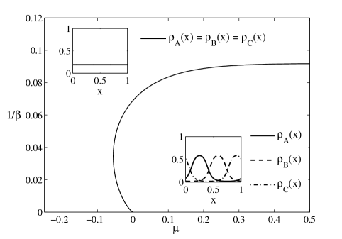
Figure 1: The $\left(\mu,\beta^{-1}\right)$ phase diagram of the generalized ABC model with conserving dynamics, displaying a second order phase transition line between a homogeneous and a phase-separated states. Typical density profile, $\rho_{n}(x)$, in each phase are given in the insets.

We now provide an alternative derivation of this phase diagram by expanding the free energy of the model in small deviations of the density profile from the homogeneous solution. This approach yields more information about the nature of the transition, and will especially be useful in the next section for analyzing the nonconserving phase diagram.

For this purpose, we turn to the continuum limit [32, 36], where the local densities of $A,\,B$ and $C$ particles at the point $x=i/L$ are represented by the density profile $\rho_{n}(x)$, $n=A,B,C$, with $\rho(x)=\rho_{A}(x)+\rho_{B}(x)+\rho_{C}(x)$. The average particle density is $r=N/L=\int_{0}^{1}\rho(x)dx$. The steady-state distribution of the density profiles may be expressed as $P\left[\rho_{n}(x)\right]=\exp\left\{-L\mathcal{F}\left[\rho_{n}(x)\right]\right\}$, where $\mathcal{F}\left[\rho_{n}(x)\right]$ is the free energy functional, rescaled by $\beta$. The equilibrium profile can thus be found by minimizing the free energy functional with respect to $\rho_{n}(x)$, under the equal densities condition, $\int_{0}^{1}\rho_{A}(x)dx=\int_{0}^{1}\rho_{B}(x)dx=\int_{0}^{1}\rho_{C}(x)dx=r/3$. The free energy functional for the conserving model is

$$\mathcal{F}[\rho_{n}(x)] = \int_{0}^{1}dx\left[\rho_{A}(x)\ln\rho_{A}(x)+\rho_{B}(x)\ln\rho_{B}(x)\right.$$ (18)

$$+ \left.\rho_{C}(x)\ln\rho_{C}(x)+\left(1-\rho(x)\right)\ln\left(1-\rho(x)\right)\right]$$

$$+ \beta\left\{\int_{0}^{1}dx\int_{0}^{1}dz\left[\rho_{A}(x)\rho_{B}(x+z)+\rho_{B}(x)\rho_{C}(x+z)\right.\right.$$

$$+ \left.\left.\rho_{C}(x)\rho_{A}(x+z)\right]z-\frac{1}{6}r^{2}\right\},$$

where the first integral corresponds to the entropy and the second integral corresponds to the continuum limit of the Hamiltonian (14).

Some characteristics of the equilibrium profile $\rho_{n}(x)$ can be determined by the symmetry of the model. Due to the cyclic boundary conditions, $\rho_{A}(x)$, $\rho_{B}(x)$ and $\rho_{C}(x)$ are periodic functions with period $1$. In addition, since the Hamiltonian favors phase separation between the three species, we expect the density profiles in the equal densities case to satisfy

$$\rho_{B}(x)=\rho_{A}\left(x-\frac{1}{3}\right)\,,\qquad\rho_{C}(x)=\rho_{A}\left(x+\frac{1}{3}\right).$$ (19)

This assumption is further justified in C. We now use the translation symmetry of the model and set $x=0$ at the symmetry axis of $\rho_{A}(x)$. The coarse grained state of the model can thus be represented by a Fourier series for $\rho_{A}(x)$

$$\rho_{A}(x) = \frac{r}{3}+\sum_{m=1}^{\infty}a_{m}\cos\left(2m\pi x\right).$$ (20)

The relation (19) implies that the other two profiles are given by

$$\rho_{B}(x) = \frac{r}{3}+\sum_{m=1}^{\infty}a_{m}\cos\left[2m\pi\left(x-\frac{1}{3}\right)\right],$$

$$\rho_{C}(x) = \frac{r}{3}+\sum_{m=1}^{\infty}a_{m}\cos\left[2m\pi\left(x+\frac{1}{3}\right)\right].$$ (21)

At high temperatures, $T=1/\beta$, all coefficients $a_{m}$ vanish, and the profile is homogeneous, with $\rho_{A}(x)=\rho_{B}(x)=\rho_{C}(x)=r/3$.

In order to find the transition line between the disordered and ordered phases we expand $\mathcal{F}$ close to the homogeneous profile in terms of a small perturbation by assuming $a_{m}\ll 1$. The amplitudes evolve by $\frac{da_{m}}{dt}=-\frac{\partial\mathcal{F}}{\partial a_{m}}$. In A we show that the transition to the inhomogeneous phase takes place at $\beta=2\pi\sqrt{3}/r$ when the first mode, $a_{1}$, becomes unstable, whereas all higher order modes are linearly stable. Just below this critical line the higher order modes ($m>1$) are driven by $a_{1}$ and may be represented by a power series of $a_{1}$. The amplitude of $a_{1}$ may thus serve as the order parameter of the transition.

The amplitudes of the higher order modes ($m>1$) are obtained by setting $\partial\mathcal{F}/\partial a_{m}=0$, which yields to lowest order $a_{m}\sim a_{1}^{m}$ (see A). The fact that the vacancies are homogeneously distributed in the equilibrium state implies that the total particle density is constant in space, $\rho_{0}(x)=1-\rho(x)=1-r$, and hence $\delta\rho_{A}(x)+\delta\rho_{B}(x)+\delta\rho_{C}(x)=0$. From this it follows that all $a_{3m}$ coefficients vanish for $m\geq 1$. Consequently, the expansion of $\mathcal{F}[\rho_{n}(x)]$ in powers of $a_{1}$ is greatly simplified. Up to order $a_{1}^{4}$ it requires terms that involve only the coefficients $a_{1}$ and $a_{2}$, yielding

$$\mathcal{F}\left[r/3+\delta\rho_{n}(x)\right]=\mathcal{F}_{{\rm h}}(r)+\left(\frac{9}{4r}-\frac{3\sqrt{3}\beta}{8\pi}\right)a_{1}^{2}$$

$$+\left(\frac{9}{4r}+\frac{3\sqrt{3}\beta}{16\pi}\right)a_{2}^{2}-\frac{27}{8r^{2}}a_{1}^{2}a_{2}+\frac{81}{32r^{3}}a_{1}^{4}+\mathcal{O}\left(a_{1}^{6}\right),$$ (22)

where $\mathcal{F}_{{\rm h}}(r)$ is the free energy of the homogeneous profile given by

$$\mathcal{F}_{{\rm h}}\left(r\right)=r\ln\left(\frac{r}{3}\right)+\left(1-r\right)\ln\left(1-r\right).$$ (23)

Details of this derivation are given in A.

We can express $a_{2}$ in terms of $a_{1}$ using the equation $\partial\mathcal{F}/\partial a_{2}=0$, which yields:

$$a_{2}=\frac{9\pi}{r\left(\sqrt{3}\beta r+12\pi\right)}a_{1}^{2}.$$ (24)

We finally obtain the following Landau expansion of the model, given by the power series of $\mathcal{F}$ in the order parameter $a_{1}$:

$$\mathcal{F}\left[\rho_{n}(x)\right]=\mathcal{F}_{h}(r)+f_{2}a_{1}^{2}+f_{4}a_{1}^{4}+\mathcal{O}\left(a_{1}^{6}\right),$$ (25)

where

$$f_{2}\left(\beta,r\right)=\frac{9}{4r}-\frac{3\sqrt{3}\beta}{8\pi},\quad f_{4}\left(\beta,r\right)=\frac{81}{32r^{3}}\left(\frac{\sqrt{3}\beta r+6\pi}{\sqrt{3}\beta r+12\pi}\right)>0.$$ (26)

By setting $f_{2}=0$ we obtain the same critical line as in Eq. (13), shown in Figure 1. The fact that $f_{4}$ is positive for any value of $r$ indicates that this is a second order transition line, from the disordered phase, where $f_{2}>0$ and $\mathcal{F}$ is minimized by $a_{1}=0$, to the ordered phase, where $f_{2}<0$, in which $\mathcal{F}$ is minimized by a nonvanishing $a_{1}$.

5 Phase diagram of the ABC model with nonconserving dynamics

5.1 The second order line

The free energy functional corresponding to the generalized ABC model with nonconserving dynamics is

$$\mathcal{G}[\rho_{n}(x)]=\mathcal{F}\left[\rho_{n}(x)\right]-\beta\mu r,$$ (27)

where $\mathcal{F}\left[\rho_{n}(x)\right]$ is given by Eq. (18). In order to find the transition between the disordered and the ordered phases, $\mathcal{G}$ may be expanded close to the homogeneous profile, as was done in the previous section in analyzing $\mathcal{F}$. Here, however, in addition to the modulation of the density profiles of $A,B$ and $C$, parameterized by $a_{m}$, deviations of the overall density, $r$, represented by $\delta r$, must be taken into account. Thus, the $A$-particle density profile close to the transition can be written as

$$\rho_{A}(x)=\frac{r}{3}+\frac{\delta r}{3}+\sum_{m=1}^{\infty}a_{m}\cos(2\pi mx),$$ (28)

where here, again, $\rho_{B}(x)=\rho_{A}(x-1/3)$ and $\rho_{C}(x)=\rho_{A}(x+1/3)$. Similarly to the conserving model, the flat profile of the vacancies implies that all $a_{3m}=0$ for $m\geq 1$. One can show that to lowest order $a_{m}\sim a_{1}^{m}$ and $\delta r\sim a_{1}^{2}$. This simplifies the expansion of $\mathcal{G}$ considerably. We carried out the expansion to eighth order in $a_{1}$, however in order to avoid lengthy expressions, we outline it here and in B only to sixth order. In B we find that

$$\mathcal{G}\left[\rho_{n}(x)\right] = \mathcal{G}_{{\rm h}}\left(r\right)+\left(\frac{9}{4r}-\frac{3\sqrt{3}\beta}{8\pi}\right)a_{1}^{2}+\left(\frac{9}{4r}+\frac{3\sqrt{3}\beta}{16\pi}\right)a_{2}^{2}$$

$$- \frac{9}{4r^{2}}a_{1}^{2}\delta r+\left(\frac{1}{2\left(1-r\right)}+\frac{1}{2r}\right)\left(\delta r\right)^{2}-\frac{27}{8r^{2}}a_{1}^{2}a_{2}$$

$$+ \frac{81}{32r^{3}}a_{1}^{4}+\frac{243}{32r^{5}}a_{1}^{6}-\frac{9}{4r^{2}}a_{2}^{2}\delta r+\frac{81}{8r^{3}}a_{1}^{2}a_{2}^{2}$$

$$+ \frac{9}{4r^{3}}a_{1}^{2}\delta r^{2}-\frac{243}{32r^{4}}a_{1}^{4}\delta r-\frac{243}{16r^{4}}a_{1}^{4}a_{2}$$

$$+ \frac{27}{4r^{3}}a_{1}^{2}a_{2}\delta r+\left(\frac{1}{6\left(1-r\right)^{2}}-\frac{1}{6r^{2}}\right)\left(\delta r\right)^{3}+\mathcal{O}\left(a_{1}^{8}\right),$$

where

$$\mathcal{G}_{{\rm h}}\left(r\right)=r\ln\left(\frac{r}{3}\right)+\left(1-r\right)\ln\left(1-r\right)-\beta\mu r$$ (30)

is the free energy of the homogeneous profile.

In order to characterize the nature of the transition line of the nonconserving model, the expansion in Eq. (5.1) has to be continued to eighth order in $a_{1}$, by taking into account terms that involve only the amplitudes $a_{1}$,$a_{2}$, $a_{4}$ and $\delta r$. The amplitudes are substituted by the following series in $a_{1}$:

$$\delta r=A_{0,2}a^{2}_{1}+A_{0,4}a^{4}_{1}+A_{0,6}a^{6}_{1}$$

$$a_{2}=A_{2,2}a^{2}_{1}+A_{2,4}a^{4}_{1}+A_{2,6}a^{6}_{1}$$

$$a_{4}=A_{4,4}a^{4}_{1}.$$ (31)

The coefficients $\{A_{i,j}\}$ are derived from the equilibrium condition $\partial\mathcal{G}/\partial\left(\delta r\right)=0$ and $\partial\mathcal{G}/\partial a_{m}=0$ for $m>1$ (see B). Thus, the Landau expansion of $\mathcal{G}$ in terms of $a_{1}$ is obtained:

$$\mathcal{G}\left[\rho_{n}(x)\right]=\mathcal{G}\left(r\right)+g_{2}a^{2}_{1}+g_{4}a^{4}_{1}+g_{6}a^{6}_{1}+g_{8}a^{8}_{1}\ldots$$ (32)

The second order coefficient

$$g_{2}\left(\beta,r\right)=f_{2}\left(\beta,r\right)=\frac{9}{4r}-\frac{3\sqrt{3}\beta}{8\pi},$$ (33)

vanishes at $\beta_{c}=2\pi\sqrt{3}/r$. On the critical line, $\beta=\beta_{c}$, the fourth order coefficient is:

$$g_{4}\left(\beta_{c},r\right)=\frac{27}{32r^{3}}\left(3r-1\right)\leavevmode\nobreak\ .$$ (34)

It is positive for $r>1/3$ and it becomes negative for $r<1/3$. Therefore, there is a multicritical point (MCP) at $r_{{\rm MCP}}=1/3$, with

$$\beta_{{\rm MCP}}=6\pi\sqrt{3}\simeq 32.648 \mu_{{\rm MCP}}=-\frac{\ln\left(6\right)}{6\pi\sqrt{3}}\simeq-0.0549.$$ (35)

Calculating the higher order coefficients, we find that on the critical line

$$g_{6}\left(\beta_{c},r\right)=\frac{81}{64r^{5}}\left(6r^{2}-5r+1\right),$$ (36)

$$g_{8}\left(\beta_{c},r\right)=\frac{27}{1024r^{7}}\left(1215r^{3}-1692r^{2}+762r-109\right).$$ (37)

The sixth order coefficient vanishes at the MCP, $g_{6}\left(\beta_{c},r_{MCP}\right)=0$. This seems to be an accidental coincidence, and it will be discussed in more detail in Section 6. The coefficient becomes negative just above the MCP. However, the eighth order coefficient is positive, $g_{8}\left(\beta_{c},r_{MCP}\right)>0$, and large enough so that the second order transition is stable above the MCP. Thus, the MCP is, in fact, a fourth order critical point. A plot of the coefficients $g_{4},g_{6}$ and $g_{8}$ along the critical line as a function of $r$ is shown in Figure 2. At low densities, $r<r_{MCP}=1/3$, $g_{4}\left(\beta_{c},r\right)$ is negative and we expect the transition to become first order.

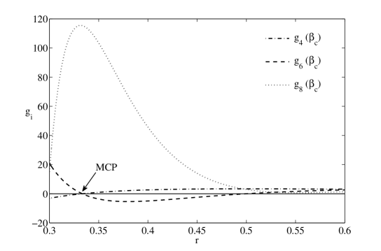
Figure 2: The 4^th,6^th and 8^th order coefficients in the expansion of $\mathcal{G}$ along the critical line. Both the 4^th and 8^th order coefficients are positive above the MCP. The 6^th order coefficient is negative just above the MCP, and vanishes at the MCP itself.

5.2 The first order line

In this section we complete the phase diagram of the nonconserving model by evaluating the first order transition below the multi-critical point. We begin by considering the behavior of the model at $1/\beta=T=0$, where the density profile has a trivial form. We then derive the first order line using an analytic expression of the mean-field profile. Finally we provide a simple approximation for the first order line at low temperatures, which also yields a lower bound for the transition for arbitrary temperature.

In the limit $1/\beta=T\to 0$, the entropy may be neglected and the free energy functional, $\mathcal{G}[\rho_{n}(x)]$, is given by the energy:

$$\mathcal{G}_{T=0}\left[\rho_{n}(x)\right]=\beta\left\{\int_{0}^{1}dx\int_{0}^{1}dz\left[\rho_{A}(x)\rho_{B}(x+z)+\rho_{B}(x)\rho_{C}(x+z)\right.\right.$$

$$\left.\left.+\rho_{C}(x)\rho_{A}(x+z)\right]z-\frac{1}{6}r^{2}-\mu r\right\}.$$ (38)

It is straightforward to verify that the ground state profile is the fully separated state,

$$\rho_{A}^{{\rm sep}}(x) = \left\{\begin{array}[]{cc}r&x<\frac{1}{3}\\ 0&{\rm otherwise}\end{array}\right.,$$ (41)

with $\rho_{B}^{{\rm sep}}(x)=\rho_{A}^{{\rm sep}}(x-1/3)$ and $\rho_{C}^{{\rm sep}}(x)=\rho_{A}^{{\rm sep}}(x+1/3)$. The free energy of this state,

$$\mathcal{G}_{T=0}(r)=-\beta\left(\frac{1}{18}r^{2}+\mu r\right),$$ (42)

is minimal at $r=0$ for $\mu<-\frac{1}{18}$ and at $r=1$ for $\mu>-\frac{1}{18}$. Consequently, there is a discontinuous transition from an empty system to a fully occupied phase-separated one at $\mu=-\frac{1}{18}$ and $T=0$. This suggests that there is a first order transition line, denoted here as $(T^{\star},\mu^{\star})$, which connects $(0,-\frac{1}{18})$ and the MCP.

The derivation of the first order transition line requires an explicit expression for the density profile, $\rho_{n}(x)$, at finite temperatures. To this end we first compute the profile of the conserving model using its mapping to the standard ABC model presented in the first paragraph of Section 4. According to this mapping, the steady state of a conserving model of size $L$ can be extracted from that of the standard ABC model (without vacancies) of size $N$ with an effective inverse temperature of $\beta r$. For the standard ABC model we can apply the analytic solution of the mean-field equations which has been suggested by Fayolle et al. [37] and derived explicitly by Ayyer et al. [36] (see also C). The solution has been formulated for the ABC model on an interval, but for the case of equal densities it applies also for periodic boundary conditions. We use it to obtain the profile at an inverse temperature $\beta r$, and map it back to the profile of the corresponding generalized model (with vacancies) by multiplying it by $r$, yielding :

$$\rho_{A}(x)=r\frac{1+\mathrm{sn}\left(2\beta rx/\varkappa,k\right)}{\alpha_{+}-\alpha_{-}\mathrm{sn}\left(2\beta rx/\varkappa,k\right)}\quad,$$ (43)

where $\mathrm{sn}$ stands for the Jacobi elliptic function, and $\varkappa,\alpha_{+},\alpha_{-},k$ are functions of the parameter $\beta r$ whose form is given in C. The profiles for $B$ and $C$ are again given as $\rho_{B}(x)=\rho_{A}(x-1/3)$ and $\rho_{C}(x)=\rho_{A}(x+1/3)$.

As shown in C the density profile in Eq. (43) is also a stationary solution of the mean-field equations of the nonconserving model. These mean-field equations include, however, an additional constraint,

$$\rho_{0}^{3}\left(x\right)=e^{-3\beta\mu}\rho_{A}\left(x\right)\rho_{B}\left(x\right)\rho_{C}\left(x\right),$$ (44)

which results from the detailed balance condition relating the evaporation and deposition processes (8). This constraint yields the relation between $\mu,r$ and $\beta$ given by

$$\mu=\frac{1}{\beta}\ln{\left[\frac{rK^{1/3}\left(\beta r\right)}{1-r}\right]},$$ (45)

where $K$ is independent of $x$, and obeys $Kr^{3}=\rho_{A}(x)\rho_{B}(x)\rho_{C}(x)$. The dependence of $K$ on the parameter $\beta r$ is given in C. Equation (45) also defines the chemical potential in the conserving model, where each steady-state profile is also a stationary solution of the nonconserving model with that value of $\mu$.

The resulting $\mu\left(r\right)$ curves for fixed $\beta$ are shown in Figure 3. The key feature is the region of $\mu$ in Figure 3b where there are 3 available solutions for $r$. The solution with the intermediate values of $r$ has negative compressibility and it is therefore unstable under the nonconserving dynamics. At the value of $\mu$ for which the two other stable solutions have the same free energy (denoted by a dashed line) the nonconserving model undergoes a first order phase transition. The transition point, $\mu^{\star}$, is found by evaluating the free energy of the nonconserving model, $\mathcal{G}$, using the chemical potential and the density profile given above. In principle, one can deduce the entire phase diagram using this nonperturbative approach. However, the expansion of the free energy in Section 5.1 is more convenient for characterizing the nature of the transition.

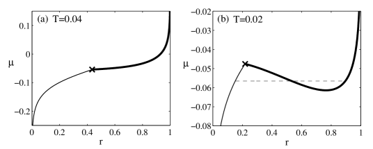
Figure 3: The $\mu(r)$ curve at constant temperature as calculated in the conserving model using the analytic solution of the mean-field equations. The thin and thick lines correspond to the homogeneous and ordered phases, respectively, and the transition point is marked by $\bf x$. In (a) $T=0.04>T_{MCP}$, while in (b) $T=0.02<T_{MCP}$. The dashed line in (b) marks the point where the free energy of the two phases is equal and the nonconserving model exhibits a first order transition.

The phase diagram of the nonconserving model with the resulting first order line is presented in Figure 4. The numerical evaluation of Eq. (43) and (45) requires numerical precision that grows linearly with $\beta=1/T$ making it prohibitive at low temperatures. To study this limit we now present a simple approximation for the transition line which also yields a lower bound for the transition at all temperatures.

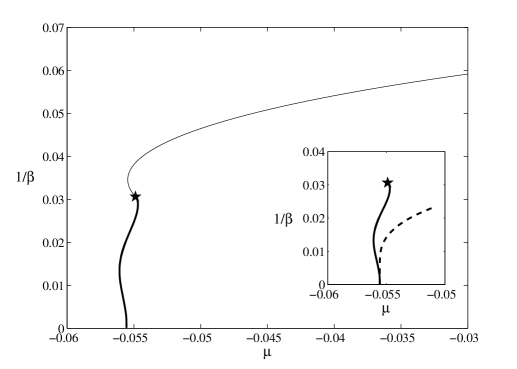
Figure 4: Phase diagram for the generalized ABC model with nonconserving dynamics. The second order (thin line) and first order (thick line) transitions are separated by a multicritical point ($\star$). The first order line terminates at ($T=0,\mu=-1/18$). The inset displays the lower bound for the first order line (dashed line) in comparison with the exact first order transition (see text).

We first observe that above the transition curve ($T>T^{\star}$ or $\mu<\mu^{\star}$) the optimal profile is homogeneous, with $\rho_{n}(x)=r/3$. The value of the average density $r$ is determined by minimizing the free energy of the homogeneous profile (30) with respect to $r$. As the model approaches the transition point, the free energy, $\mathcal{G}$, develops a local minimum corresponding to a inhomogeneous density profile. The transition temperature may be defined as the lowest temperature for which the free energy of the homogeneous profile is lower than that of any other profile. Instead of considering any possible profile, we look at the totally separated profile in Eq. (41), whose corresponding free energy is given by

$$\mathcal{G}_{{\rm sep}}(r)=r\ln\left(r\right)+\left(1-r\right)\ln\left(1-r\right)-\beta\left(\frac{1}{18}r^{2}+\mu r\right).$$ (46)

For $T>0$ the model eventually displays an ordered phase that is not fully separated and therefore has a lower free energy (due to entropic effects) than $\mathcal{G}_{{\rm sep}}(r)$. Hence, for a given $\mu$ the temperature at which

$$\min_{r}\mathcal{G}_{{\rm h}}(r)=\min_{r}\mathcal{G}_{{\rm sep}}(r),$$ (47)

is a lower bound for the transition temperature, $T^{\star}$. At low temperatures, the first order transition line approaches this lower bound and the ordered profile is well represented by the fully phase-separated one. Thus, this bound provides a good approximation for the behavior of the system at low temperatures ($T\ll T_{MCP}$), as shown in the inset of Figure 4.

5.3 Monte Carlo simulations

The picture emerging from the continuum limit is supported by the results of Monte Carlo (MC) simulations, performed under effective equilibrium conditions, $N_{A}=N_{B}=N_{C}=N/3$, with both conserving and nonconserving dynamics.

In the nonconserving simulations, the state of the system is updated according to the following procedure: At each time-step a single site is randomly selected. The type of move to attempt is also chosen randomly: with probability $1/2$ an attempt is made to exchange the particle of the chosen site with its right-hand neighbor and with probability $1/2$ an evaporation or deposition process is attempted. In the latter case, if the chosen site is occupied by a $B$ particle with an $A$ to its left and a $C$ to its right, then the removal of the triplet $ABC$ is attempted. If the chosen site is vacant, and it is surrounded on both sides by vacant sites as well, the condensation of an $ABC$ triplet is attempted. Finally, the move is accepted with probability

$$P=\left\{\begin{array}[]{cc}\exp\left(-\beta\frac{\Delta\mathcal{H}_{GC}}{L}\right)&\Delta\mathcal{H}_{GC}>0\\ 1&{\rm otherwise}\end{array}\right.,$$ (48)

where $\Delta\mathcal{H}_{GC}$ is the change in energy due to the chosen move, as determined by Eq. (10) (possible values are $0$, $\pm 1$ and $\pm 3\mu L$). This procedure leads to a steady state which obeys detailed balance with respect to the nonconserving Hamiltonian (10).

In order to compare the results of these simulations with those of the conserving simulations one has to calculate the chemical potential, $\mu$, for a given temperature under conserving dynamics. This can be done by employing in the conserving simulations a method similar to the Creutz algorithm for microcanonical MC simulations [39]. The idea is to perform a constrained nonconserving simulation so that the average density, $r$, is allowed to fluctuate only below its initial value, $r(0)$, while extracting the value of $\mu$ from these fluctuations. The simulation is executed as in the nonconserving case by selecting a site and an attempted move. Steps in which neighboring particles are exchanged are accepted according to Eq. (48). The particle nonconserving steps are performed in conjunction with an additional single degree of freedom, termed ’demon’, that exchanges particles with the system. The ’demon’ is initially empty. An attempt of removing $ABC$ triplet is accepted with probability $1$, and the removed particles are added to the ’demon’. Steps that require the deposition of an $ABC$ triplet on three vacant sites are accepted only if the ’demon’ is not vacant and with a rate given by Eq. (48) with $\mathcal{H}_{GC}$ replaced by the canonical Hamiltonian, $\mathcal{H}_{C}$ (14). The triplet is then removed from the ’demon’. As a result the average density is allowed to fluctuate, but only to states with an average density below $r(0)$. Fluctuations with higher densities are rejected. In the thermodynamic limit this procedure yields the canonical distribution of the system with density $r(0)$, even for systems with negative compressibility [20]. The probability distribution of the number of particles in the ’demon’, $P\left(N_{demon}\right)$, is recorded during the simulation. The chemical potential, $\mu$, is determined from this distribution using the equilibrium relation $P\left(N_{demon}\right)\sim\exp\left(-\beta\mu N_{demon}\right)$. A typical distribution is given in Figure 5, from which $\mu$ is extracted by applying a linear fit to $\ln\left[P\left(N_{demon}\right)\right]$.

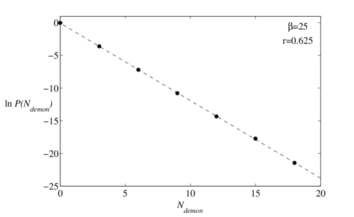
Figure 5: Natural logarithm of the probability distribution of the ’demon’ occupation number as obtained by MC simulations of the conserving dynamics for $L=1800$, $N=1125$ and $\beta=25$. Linear fit (dashed line) of the simulation points yields $\mu\simeq 0.047$. Such simulations yield the $\mu(r)$ curve.

The simulation results are displayed and compared with the mean-field solution (45) in Figure 6, where the average density, $r$, is plotted as a function of the chemical potential, $\mu$. Above the multicritical point, in Figure 6a, we see that the conserving and nonconserving simulations follow the same curve. The two types of dynamics are thus equivalent, and undergo a second order transition at the critical point (17) marked in the figure by x. Below the multicritical point, in Figure 6b, the conserving simulation exhibits a similar second order transition, whereas the nonconserving simulation shows a discontinuity in $r$. At the intermediate-density states we find negative compressibility in the conserving simulation. These states are unstable under the nonconserving dynamics, where $r$ can fluctuate freely. The nonconserving model thus exhibits a discontinuity in $r$, accompanied by hysteretic behavior. This hysteresis is an indication of the first order transition. The value of $\mu$ at the transition, as found in the thermodynamic limit using the analytical procedure discussed in Section 5.2, is denoted by the dashed line. This thus provides a direct observation of the inequivalence of two ensembles. The results of the simulations fit very well the mean-field solution (45).

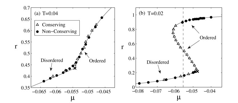
Figure 6: The $\mu(r)$ curve of the conserving ($\triangle$) and nonconserving ($\bullet$) dynamics obtained by direct simulations for $L=1800$. The simulations were performed at two temperatures (a) $T=0.04$, above the MCP, and (b) $T=0.02$, below the MCP ($T_{{\rm MCP}}\simeq 0.03$). In (a) both the conserving ($\triangle$) and nonconserving ($\bullet$) simulations result in the same curve within the numerical accuracy. In (b) the two types of dynamics yield different curves, with the nonconserving dynamics displaying a discontinuity in r at a first order transition. Hysteretic behavior is observed in the nonconserving case. The expected first order transition point, obtained by minimization of $\mathcal{G}$, is indicated by the dashed vertical line. The solid lines correspond to the analytic solution of the mean field equations and so is the x, which denotes the second order transition point in conserving model.

6 Further generalization of the model

The nonconserving ABC model with equal densities exhibits a seemingly accidental coincidence whereby the sixth order coefficient in the expansion of the free energy vanishes at the MCP, i.e. $g_{2}=g_{4}=g_{6}=0$. If indeed this feature is accidental one expects any modification of the model to remove this degeneracy. In this section we consider a simple generalization of the nonconserving dynamics that maintains detailed balance under the equal densities condition. Thus, the features of the phase diagram may be found using the expansion of free energy functionals, as presented in the previous sections.

The generalization consists of replacing the factor $1/6$ in the Hamiltonian in Eq. (10) by a free parameter $\gamma$,

$$\mathcal{H}_{GC,\gamma}\left(\left\{X_{i}\right\}\right)=\mathcal{H}\left(\left\{X_{i}\right\}\right)-\gamma N\left(N-1\right)-\mu NL,$$ (49)

where $\mathcal{H}\left(\left\{X_{i}\right\}\right)$ is given by Eqs. (4) or (5) . By imposing the condition for detailed balance with respect to the distribution $P_{\gamma}\left(\left\{X_{i}\right\}\right)=q^{\mathcal{H}_{GC,\gamma}\left(\left\{X_{i}\right\}\right)}/Z_{L}$ for systems with equal densities $N_{A}=N_{B}=N_{C}$, and reversing the argument of Eq. (11), we find that detailed balance is maintained for the following evaporation and deposition rates:

$$ABC\overset{pq^{\Delta\mathcal{H}_{GC,\gamma}}}{\underset{p}{\rightleftarrows}}000,$$ (50)

where

$$\Delta\mathcal{H}_{GC,\gamma}=3\mu L-\left(N+1\right)\left(1-6\gamma\right).$$ (51)

Thus the non conserving dynamics corresponding to the modified Hamiltonian (49) consists of the processes (1), (7) and (50). For $\gamma\neq 1/6$ the evaporation rate depends on the particle number, $N$, and therefore the dynamics is nonlocal.

We now analyze the phase diagram corresponding to this generalized model in the limit of weak asymmetry, $q=\exp\left(-\beta/L\right)$. The continuum-limit calculation of the phase diagram can be repeated, producing Landau expansions of the free energy functionals $\mathcal{F}_{\gamma}$ and $\mathcal{G}_{\gamma}$. In the conserving dynamics the particle number $N$ is a constant, and hence the $\gamma$-term has no effect on the expansion of $\mathcal{F}_{\gamma}$. Therefore, regardless of $\gamma$, the conserving model exhibits a second order transition at $\beta_{c}=2\pi\sqrt{3}/r$.

The expansion of $\mathcal{G}_{\gamma}$, as detailed in B, is given by,

$$\mathcal{G}_{\gamma}\left[\rho_{n}(x)\right]=\mathcal{G}_{\gamma}\left(r\right)+g_{2}^{\gamma}a^{2}_{1}+g_{4}^{\gamma}a^{4}_{1}+g_{6}^{\gamma}a^{6}_{1}+g_{8}^{\gamma}a^{8}_{1}+\ldots,$$ (52)

where $g_{2}^{\gamma}=g_{2}$ is independent of $\gamma$. It vanishes on the critical line $\beta=\beta_{c}=2\pi\sqrt{3}/r$. On this line the fourth order coefficient is given by

$$g_{4}^{\gamma}\left(\beta_{c},r\right)=\frac{27}{32r^{3}}\left[\frac{9r-3+4\pi\sqrt{3}\left(1-6\gamma\right)\left(1-r\right)}{3+2\pi\sqrt{3}\left(1-6\gamma\right)\left(1-r\right)}\right],$$ (53)

which is positive at all densities satisfying

$$r>r_{{\rm MCP}}=\frac{\sqrt{3}-4\pi\left(1-6\gamma\right)}{3\sqrt{3}-4\pi\left(1-6\gamma\right)}.$$ (54)

The coefficient vanishes at $r=r_{MCP}$ which yields:

$$\beta_{{\rm MCP}} = \frac{6\pi\left[3\sqrt{3}-4\pi(1-6\gamma)\right]}{3-4\pi\sqrt{3}(1-6\gamma)}$$

$$\mu_{{\rm MCP}} = \frac{1}{6}\left[3-4\pi\sqrt{3}(1-6\gamma)\right]\times$$ (55)

$$\left\{\frac{2(1-6\gamma)}{9-4\pi\sqrt{3}(1-6\gamma)}+\frac{\ln\left[\frac{1}{18}\left(3-4\pi\sqrt{3}(1-6\gamma)\right)\right]}{\pi\left(3\sqrt{3}-4\pi(1-6\gamma)\right)}\right\}.$$

Note that as $\gamma\rightarrow\left(4\pi-\sqrt{3}\right)/24\pi\simeq 0.144$ (from above), the density $r_{{\rm MCP}}$ vanishes, and $g_{4}$ is positive for all values of $0<r\leq 1$.

The phase diagram in the vicinity of the MCP depends strongly on the sign of the sixth order coefficient, $g_{6}^{\gamma}$, at the MCP where $g_{2}^{\gamma}=g_{4}^{\gamma}=0$. From the expansion of $\mathcal{G}_{\gamma}$ we find

$$\left(g_{6}^{\gamma}\right)_{{\rm MCP}}=\frac{\sqrt{3}\pi\left(1-6\gamma\right)\left[3-2\sqrt{3}\pi\left(1-6\gamma\right)\right]\left[4\sqrt{3}\pi\left(1-6\gamma\right)-9\right]^{5}}{8\left[3-4\sqrt{3}\pi\left(1-6\gamma\right)\right]^{5}},$$ (56)

For $\gamma>\frac{1}{6}$, one has $\left(g_{6}^{\gamma}\right)_{{\rm MCP}}>0$, and the MCP is a tricritical point (TCP). Thus, the phase diagram in this case consists of a second order line which becomes first order below the TCP. However for $\gamma<\frac{1}{6}$, the coefficient $\left(g_{6}^{\gamma}\right)_{{\rm MCP}}$ is negative and the trictitical point is unstable. As a result the first order line intersects the second order line above the TCP. Thus the phase diagram consists of a critical line which terminates at a first order line at a critical end point (CEP) where $g_{2}^{\gamma}=0,\,g_{4}^{\gamma}>0\,$ and $g_{6}^{\gamma}<0$. This point is located above the TCP (which is unstable). The first order line continues into the ordered phase, and it ends at a critical point (CP), as shown schematically in Figure 7. Above the CEP the first order line marks a transition between two ordered phases with low (I) and high (II) densities. As $\gamma$ approaches $1/6$ from below, the CEP, CP and TCP approach each other. They merge at $\gamma=1/6$, yielding a fourth order critical point.

To complete the analysis of the phase diagram one has to determine the first order line. This can be done by using the exact solution for the density profiles, as discussed in Section 5.2. The location of the first order transition at $T\to 0$ can be derived by equating the free energies of the homogeneous and the fully phase-separated states

$$\min_{r}\mathcal{G}_{\gamma,{\rm h}}(r)=\min_{r}\mathcal{G}_{\gamma,{\rm sep}}(r),$$ (57)

where

$$\mathcal{G}_{\gamma,{\rm h}}(r)=r\ln\left(\frac{r}{3}\right)+\left(1-r\right)\ln\left(1-r\right)+\beta\left(\frac{1}{6}-\gamma\right)r^{2}-\beta\mu r,$$ (58)

and

$$\mathcal{G}_{\gamma,{\rm sep}}(r)=r\ln\left(r\right)+\left(1-r\right)\ln\left(1-r\right)+\beta\left(\frac{1}{9}-\gamma\right)r^{2}-\beta\mu r.$$ (59)

At $T=0$ the model exhibits a discontinuity in the total density from $r=0$ to $r=1$ at $\mu=1/9-\gamma$, and thus undergoes a first order transition at that point.

Figure 7 shows a schematic representation of the phase diagrams of the generalized ABC model with nonlocal dynamics for conserving and nonconserving dynamics above and below $\gamma=1/6$. As expected, the nongeneric feature of a fourth order critical point has been removed by slight modification of the model. Generically, we expect the multicritical point to become either a tricritical point or a critical end point, as shown in the figure.

Figure 7: Schematic phase diagrams of the modified nonconserving ABC model with nonlocal dynamics for (a) $\gamma\geq\frac{1}{6}$ and (b) $\gamma<\frac{1}{6}$. In both cases the phase diagram is composed of a second order transition (thin line) at high temperatures, which becomes first order (thick line) at low temperatures. The dashed line marks the continuation of the second order line, which is unstable for the nonconserving dynamics. The first order line intersects the $T=0$ axis at $\mu=\frac{1}{9}-\gamma$. In (a) The two lines meet at a tricritical point (TCP), as in the local dynamics case, $\gamma=\frac{1}{6}$. On the other hand in (b) the first order transition line intersects the second order line at a critical end point (CEP). The second order line terminates at this point while the first order line continues into the ordered phase, where it marks a transition between two distinct phase-separated states, with low (I) and high (II) densities, and terminates at a critical point (CP). The hollow point on the unstable second order line, denotes the TCP where $g_{2}=g_{4}=0$ and $g_{6}<0$. This point and the dashed segment of the second order line are preempted by the first order line and are thus not accessible within the nonconserving dynamics. For particles conserving dynamics the phase diagram exhibits a second order line, composed of the thin and dashed lines in the figure, for any value of $\gamma$.

7 Conclusions

In this paper we generalized the ABC model to include vacancies and processes that do not conserve the particle number. This enables us to analyze and compare the phase diagrams of the conserving and the nonconserving models. We have shown that in the case where the average densities of the three species are equal, the dynamics of the generalized model obeys detailed balance with respect to a Hamiltonian with long-range interactions, despite the fact that the dynamics is local. Studying the $\left(\mu,T\right)$ phase diagrams of the model for equal densities, we found that in the conserving case it is composed of a second order line separating the homogeneous and phase-separated states, while in the nonconserving case the second order line becomes first order at low temperatures. The analysis of the phase diagram has been carried out by studying the Helmholtz and Gibbs free energies for the conserving and nonconserving dynamics, respectively, in the continuum limit. As has been shown in the past this limit yields the exact steady states in the thermodynamic limit. In this study we applied a critical expansion of the free energy near the homogeneous phase and an exact solution of the mean-field equations for the density profiles of the phase-separated state. The results of this analysis are verified by direct Monte Carlo simulations of the two types of dynamics.

The fact that the two types of dynamics result in rather different phase diagrams can be associated with the inequivalence of the canonical (conserving) and grand-canonical (nonconserving) ensembles in systems with long-range interactions. We find that as expected from studies of long-range interacting systems, the two ensembles yield different steady states in the region where the grand canonical ensemble displays a first order transition.

We expect the generalized ABC model to display similar behavior even for small deviations from the equal densities case, where detailed balance is not satisfied. The present study can thus serve as a starting point for a study of the ABC model out of equilibrium. It could provide an interesting correspondence between some properties of the well-understood equilibrium systems with long-range interactions and those of the less well-understood nonequilibrium driven models. Details of a study of the generalized ABC model with unequal densities will be published elsewhere [40]. An interesting driven model where ensemble-inequivalence has recently been observed is the zero-range process [41]. In this model, the drive, provided by the spatial asymmetry of the transition rates, does not influence the steady state. This state thus remains the same as the steady state of the nondriven equilibrium model, where the transition rates are symmetric, which can be expressed in terms of a Hamiltonian. By contrast, the ABC model provides a framework within which one can readily probe nonequilibrium steady states which are not expressed by a Hamiltonian.

Appendix A Critical expansion of the conserving free energy

We present the critical expansion of the free energy of the conserving model. In the continumm limit, the free energy, rescaled by $\beta$, is given by $\mathcal{F}=\beta\epsilon-s$, where

$$s\left[\rho_{n}(x)\right] = -\int_{0}^{1}dx\left[\rho_{A}(x)\ln\left(\rho_{A}(x)\right)+\rho_{B}(x)\ln\left(\rho_{B}(x)\right)\right.$$ (60)

$$\left.+\rho_{C}(x)\ln\left(\rho_{C}(x)\right)+\left(1-\rho(x)\right)\ln\left(1-\rho(x)\right)\right]$$

is the entropy per site of the profile, derived from simple combinatorial considerations, and

$$\epsilon\left[\rho_{n}(x)\right] = \int_{0}^{1}dx\int_{0}^{1}dz\left[\rho_{A}(x)\rho_{B}(x+z)+\rho_{B}(x)\rho_{C}(x+z)\right.$$ (61)

$$\left.+\rho_{C}(x)\rho_{A}(x+z)\right]z-\frac{1}{6}r^{2}$$

is the energy per site given continuum limit of the conserving Hamiltonian (14), for $n=A,B$ or $C$.

We begin by expanding the steady-state profile close the homogeneous solution in the most general form :

$$\rho_{n}(x)=\frac{r}{3}+\delta\rho_{n}(x)=\frac{r}{3}+\sum_{m=-\infty}^{\infty}\alpha_{n,m}e^{2m\pi ix}.$$ (62)

For the profile to be real we assume $\alpha_{n,-m}=\alpha_{n,m}^{\star}$. The time evolution of these modes is set by $\frac{d\alpha_{n,m}}{dt}=-\frac{\partial\mathcal{F}}{\partial\alpha_{n,-m}}$ which yields to lowest order in $\alpha_{n,m}$:

$$\frac{d}{dt}\vec{\alpha}_{m}=\left[\frac{i\beta}{2\pi m}\left(\begin{array}[]{ccc}0&1&-1\\ -1&0&1\\ 1&-1&0\end{array}\right)-\frac{3}{r}I\right]\vec{\alpha}_{m},$$ (63)

where $\vec{\alpha}_{m}=(\alpha_{A,m},\alpha_{B,m},\alpha_{C,m})$ and $I$ is the $3\times 3$ unit matrix. For the $m^{th}$ mode, the highest eigenvalue of the matrix above is $\frac{\beta\sqrt{3}}{2\pi m}-\frac{3}{r}$ with the eigenvector $(1,e^{-2\pi i/3},e^{2\pi i/3})$. As the temperature is decreased ($\beta$ increased) the first mode to become unstable is $m=1$ (at $\beta=2\pi\sqrt{3}/r$), while the other modes are linearly stable. Just below this transition line the higher modes ($m>1$) are driven by the $m=1$ mode. The $m^{th}$ mode is driven to lowest order by a term of the form $\alpha_{n,1}^{m}\alpha_{n,-m}$ in the Taylor expansion of the logarithmic function in the entropy. We thus obtain to lowest order $\alpha_{n,m}\sim\alpha_{n,1}^{m}$ with the eigenvector $(1,e^{-2m\pi i/3},e^{2m\pi i/3})$. We can therefore simplify our expansion and set

$$\rho_{A}(x)=\frac{r}{3}+\delta\rho_{A}(x)=\frac{r}{3}+\sum_{m=1}^{\infty}a_{m}\cos(2m\pi x),$$ (64)

with $\rho_{B}(x)=\rho_{A}(x-1/3)$ and $\rho_{C}(x)=\rho_{A}(x+1/3)$. This latter form is also justified in the work of Ayyer et al. [36], who proved that the ordered profile of the model is unique and obeys this symmetry.

As explained in Section 4, the flat profile of the vacancies implies that $\delta\rho_{0}=-(\delta\rho_{A}+\delta\rho_{B}+\delta\rho_{C})=0$ and therefore $a_{3m}=0$. We wish to evaluate the free energy up to order $a_{1}^{4}$ and thus expand the entropy and energy only in terms of $a_{1}$ and $a_{2}$.

The entropy of the $A$ particles is given by the first term in the RHS of Eq. (60) :

$$s_{A}=-\int_{0}^{1}dx\left[\frac{r}{3}+\delta\rho_{A}(x)\right]\ln\left[\frac{r}{3}+\delta\rho_{A}(x)\right]=$$

$$\int_{0}^{1}dx\left\{\frac{r}{3}\ln\left(\frac{r}{3}\right)+\left[1+\ln\left(\frac{r}{3}\right)\right]\delta\rho_{A}(x)+\frac{3}{2\rho}\left(\delta\rho_{A}(x)\right)^{2}\right.$$

$$\left.-\frac{3}{2\rho^{2}}\left(\delta\rho_{A}(x)\right)^{3}+\frac{9}{4\rho^{3}}\left(\delta\rho_{A}(x)\right)^{4}\right\}+\mathcal{O}\left(\delta\rho_{A}(x)\right)^{5}.$$ (65)

After performing the integral we obtain:

$$-s_{A} = \frac{r}{3}\ln\left(\frac{r}{3}\right)+a_{1}^{2}\left(\frac{3}{4r}\right)+a_{2}^{2}\left(\frac{3}{4r}\right)$$ (66)

$$+ a_{1}^{4}\left(\frac{27}{32r^{3}}\right)-a_{1}^{2}a_{2}\left(\frac{9}{8r^{2}}\right).$$

Under the condition of equal densities one has $s_{A}=s_{B}=s_{C}$, and therefore the total entropy of the particles is equal to $3s_{A}$. The total particle density is constant in space, $\rho(x)=r$, and thus the entropy of the vacancies, $\left(1-r\right)\ln\left(1-r\right)$, contributes a constant term to the expansion. The total entropy of the system is thus:

$$-s = r\ln\left(\frac{r}{3}\right)+\left(1-r\right)\ln\left(1-r\right)+a_{1}^{2}\left(\frac{9}{4r}\right)$$ (67)

$$+a_{2}^{2}\left(\frac{9}{4r}\right)+a_{1}^{4}\left(\frac{81}{32r^{3}}\right)-a_{1}^{2}a_{2}\left(\frac{27}{8r^{2}}\right).$$

Similarly in the expansion of the energy, $\epsilon$, we consider the interaction energy of A and B particles given by the first term in the RHS of Eq. (61):

$$\epsilon_{AB}=\frac{r^{2}}{18}-\frac{\sqrt{3}}{8\pi}a_{1}^{2}+\frac{\sqrt{3}}{16\pi}a_{2}^{2}.$$ (68)

From symmetry, $\epsilon_{AB}=\epsilon_{BC}=\epsilon_{CA}$. Adding the constant term $-r^{2}/6$, we find:

$$\epsilon = -a_{1}^{2}\left(\frac{3\sqrt{3}}{8\pi}\right)+a_{2}^{2}\left(\frac{3\sqrt{3}}{16\pi}\right).$$ (69)

The critical expansion of the free energy in Eq. (22) is then obtained by inserting Eqs. (67) and (69) into $\mathcal{F}=\beta\epsilon-s$.

Appendix B Critical expansion of the nonconserving free energy

We present the critical expansion of the free energy of the nonconserving model whose Hamiltonian (49) is given by

$$\mathcal{H}_{GC,\gamma}\left(\left\{X_{i}\right\}\right)=\mathcal{H}\left(\left\{X_{i}\right\}\right)-\gamma N\left(N-1\right)-\mu NL.$$ (70)

This is a modified Hamiltonian for the case of nonlocal dynamics (see Secition 6). It reduces to the Hamiltonian (10) considered in Section 5 by setting $\gamma=\frac{1}{6}$. The free energy of the model is thus

$$\mathcal{G}_{\gamma}\left[\rho_{n}(x)\right]=\beta\left[\epsilon\left[\rho_{n}(x)\right]+\left(\frac{1}{6}-\gamma\right)r^{2}-\mu r\right]-s\left[\rho_{n}(x)\right],$$ (71)

where entropy and energy, $s$ and $\epsilon$, are given in Eqs. (60) and (61) respectively. We follow the same expansion procedure presented in A, where the free energy is written as a power series of $a_{1}$. The analysis of the multi-critical point of the nonconserving phase diagram requires terms up to order $a_{1}^{8}$. We carried out the calculation to this order. However, in order to avoid lengthy expressions, we present it here only up to order $a_{1}^{6}$, where the free energy is expanded in terms that involve only the amplitudes $a_{1}$ and $a_{2}$. Here we also take into account fluctuations in the total particle density, $r$, denoted by $\delta r$. The density profile is thus expressed by the Fourier expansion,

$$\rho_{A}(x)=\frac{r}{3}+\frac{\delta r}{3}+a_{1}\cos\left(2\pi x\right)+a_{2}\cos\left(4\pi x\right).$$ (72)

The calculation is similar to that detailed in A, with some modifications. First, the dependence of the entropy of the vacancies on the density, and thus on $\delta r$, has to be taken in to account. It takes the form:

$$-s_{0} = \left(1-r\right)\ln\left(1-r\right)-\delta r\left[1+\ln\left(1-r\right)\right]$$ (73)

$$+ \frac{\left(\delta r\right)^{2}}{2\left(1-r\right)}+\frac{\left(\delta r\right)^{3}}{6\left(1-r\right)^{2}}.$$

In addition, the density in the homogeneous steady state depends on the value of $\mu$ and is determined by the equilibrium condition:

$$\frac{\partial}{\partial r}\mathcal{G}_{\gamma,{\rm h}}\left(r\right)=\ln\left(\frac{r}{3\left(1-r\right)}\right)+2\beta\left(\frac{1}{6}-\gamma\right)r-\beta\mu=0,$$ (74)

where $\mathcal{G}_{\gamma,{\rm h}}$ is the free energy of the homogeneous profile (58). The expansion of the free energy is:

$$\mathcal{G}_{\gamma}\left[\rho_{n}(x)\right] = \mathcal{G}_{\gamma,{\rm h}}\left(r\right)+\left(\frac{9}{4r}-\frac{3\sqrt{3}\beta}{8\pi}\right)a_{1}^{2}+\left(\frac{9}{4r}+\frac{3\sqrt{3}\beta}{16\pi}\right)a_{2}^{2}$$

$$- \frac{9}{4r^{2}}a_{1}^{2}\delta r+\left(\frac{\beta}{6}-\beta\gamma+\frac{1}{2\left(1-r\right)}+\frac{1}{2r}\right)\left(\delta r\right)^{2}-\frac{27}{8r^{2}}a_{1}^{2}a_{2}$$

$$+ \frac{81}{32r^{3}}a_{1}^{4}+\frac{243}{32r^{5}}a_{1}^{6}-\frac{9}{4r^{2}}a_{2}^{2}\delta r+\frac{81}{8r^{3}}a_{1}^{2}a_{2}^{2}$$

$$+ \frac{9}{4r^{3}}a_{1}^{2}\delta r^{2}-\frac{243}{32r^{4}}a_{1}^{4}\delta r-\frac{243}{16r^{4}}a_{1}^{4}a_{2}$$

$$+ \frac{27}{4r^{3}}a_{1}^{2}a_{2}\delta r+\left(\frac{1}{6\left(1-r\right)^{2}}-\frac{1}{6r^{2}}\right)\left(\delta r\right)^{3}+\mathcal{O}\left(a_{1}^{8}\right),$$

We use the following expansion for the amplitudes:

$$\delta r=A_{0,2}a^{2}_{1}+A_{0,4}a^{4}_{1},\quad a_{2}=A_{2,2}a^{2}_{1}+A_{2,4}a^{4}_{1}.$$ (76)

Substituting these terms in $\mathcal{G}$ results in the power series:

$$\mathcal{G}_{\gamma}\left[\rho_{n}(x)\right]=\mathcal{G}_{\gamma,h}\left(r\right)+g_{2}^{\gamma}a^{2}_{1}+g_{4}^{\gamma}a^{4}_{1}+g_{6}^{\gamma}a^{6}_{1}+\mathcal{O}\left(a^{8}_{1}\right),$$ (77)

where

$$g_{2}^{\gamma}=\frac{9}{4r}-\frac{3\sqrt{3}\beta}{8\pi},$$ (78)

and

$$g_{4}^{\gamma}=\frac{81}{32r^{3}}-\frac{27}{8r^{2}}A_{2,2}-\frac{9}{4r^{2}}A_{0,2}$$

$$+\left(\frac{3\sqrt{3}\beta}{16\pi}+\frac{9}{4r}\right)A_{2,2}^{2}+\left(\frac{\beta}{6}-\beta\gamma+\frac{1}{2r(1-r)}\right)A_{0,2}^{2}.$$ (79)

The coefficient $g_{6}^{\gamma}$ can be expressed in a similar fashion.

The coefficients $\left\{A_{i,j}\right\}$ are derived from the equilibrium condition:

$$\frac{\partial\mathcal{G}_{\gamma}\left[\rho_{n}(x)\right]}{\partial a_{2}}=0\,,\qquad\frac{\partial\mathcal{G}_{\gamma}\left[\rho_{n}(x)\right]}{\partial\left(\delta r\right)}=0.$$ (80)

Expanding the equation for $a_{2}$ in powers of $a_{1}$ and using Eq. (76), we find

$$0=\left(\frac{3\sqrt{3}\beta}{8\pi}A_{2,2}-\frac{27}{8r^{2}}+\frac{9}{2r}A_{2,2}\right)a^{2}_{1}$$

$$+\frac{3}{16\pi r^{4}}\left(-81\pi+108A_{2,2}\pi r+36A_{0,2}\pi r-24A_{2,2}A_{0,2}\pi r^{2}\right.$$

$$\left.+24A_{2,4}\pi r^{3}+2\sqrt{3}\beta A_{2,4}r^{4}\right)a^{4}_{1}+\ldots$$ (81)

Each power of $a_{1}$ has to be equal to zero independently. From the second order term, we find

$$A_{2,2}=\frac{9\pi}{r\left(12\pi+\sqrt{3}\beta r\right)}.$$ (82)

Similarly, expanding the equation $\partial\mathcal{G}_{\gamma}/\partial\left(\delta r\right)=0$ in powers of $a_{1}$ one finds

$$A_{0,2}=\frac{27\left(1-r\right)}{4r\left[3+\beta r\left(1-r\right)\left(1-6\gamma\right)\right]}.$$ (83)

Equations (82) and (83) are then used to evaluate $A_{2,4}$ from the fourth order term in (81):

$$A_{2,4}=\frac{81\pi}{2r^{3}\left(12\pi+\sqrt{3}\beta r\right)^{2}}\times$$

$$\frac{\sqrt{3}\beta r^{2}\left[3+\beta(1-r)(1-6\gamma)\right]-18\pi(1-r)}{3+\beta r\left(1-r\right)\left(1-6\gamma\right)}.$$ (84)

The higher order coefficients are found in a similar manner.

Substituting the coefficients in the expression for the free energy $\mathcal{G}_{\gamma}$, we obtain

$$g_{4}^{\gamma}=\frac{81}{32r^{3}}\left[\frac{\sqrt{3}\beta r+6\pi}{\sqrt{3}\beta r+12\pi}-\frac{3\left(1-r\right)}{3+\beta\rho\left(1-r\right)\left(1-6\gamma\right)}\right].$$ (85)

To avoid lengthy expressions we display the expression for $g_{6}$ only along the critical line $\beta_{c}=2\pi\sqrt{3}/r$. With the notation $\theta=\left(1-r\right)\left(1-6\gamma\right)$ it is given by:

$$g_{6}^{\gamma}\left(\beta_{c}\right)=\frac{243}{64r^{5}\left[3+2\pi\sqrt{3}\theta\right]^{3}}\times$$

$$\left[16\pi^{3}\sqrt{3}\theta^{3}+6\pi^{2}\theta^{2}\left(17r-5\right)\right.$$

$$\left.+6\pi\sqrt{3}\theta\left(9r^{2}-r-2\right)+9\left(6r^{2}-5r+1\right)\right].$$ (86)

For $\gamma=\frac{1}{6}$ we find that at the multicritical point, where $g_{2}^{\gamma}=g_{4}^{\gamma}=0$, one also has $g_{6}^{\gamma}=0$. We therefore need to calculate the eighth-order coefficient, $g_{8}^{\gamma}$, in the same manner described above. This requires the evaluation of the amplitude $a_{4}$ as well. This calculation, whose details are not presented here, yields the following expression for $g_{8}^{\gamma}$ along the critical line

$$g_{8}^{\gamma}\left(\beta_{c}\right)=\frac{243}{1024r^{7}\left[3+2\pi\sqrt{3}\theta\right]^{5}}\times$$

$$\left[5632\pi^{5}\sqrt{3}\theta^{5}+24\pi^{4}\theta^{4}\left(2883r-1123\right)\right.$$

$$+48\pi^{3}\sqrt{3}\theta^{3}\left(1800r^{2}-717r-203\right)$$

$$+72\pi^{2}\theta^{2}\left(1458r^{3}+567r^{2}-1413r+268\right)$$

$$+18\pi\sqrt{3}\theta\left(3645r^{3}-3186r^{2}+204r+217\right)$$

$$\left.+27\left(1215r^{3}-1692r^{2}+762r-109\right)\right].$$ (87)

The coefficient $g_{4}^{\gamma},g_{6}^{\gamma}$ and $g_{8}^{\gamma}$ are used for the expansion of the free energy for $\gamma=\frac{1}{6}$ in Eq. (32) and for $\gamma\neq\frac{1}{6}$ in Eq. (52).

Appendix C Steady-state profiles in the continuum limit

In order to locate the first order transition line of the ABC model one has to calculate the density profiles of the three species in the ordered phase. In this Appendix we provide an analytic solution for the profiles by applying the approach introduced in [36]. This is done first by translating the dynamical rules in Eq. (1) to an equation for the time evolution of $\left\langle A_{i}\right\rangle$ as

$$\frac{d}{dt}\left\langle A_{i}\right\rangle=q\left\langle A_{i-1}B_{i}\right\rangle+q\left\langle C_{i}A_{i+1}\right\rangle+\left\langle B_{i}A_{i+1}\right\rangle+\left\langle A_{i-1}C_{i}\right\rangle$$

$$-q\left\langle A_{i}B_{i+1}\right\rangle-q\left\langle C_{i-1}A_{i}\right\rangle-\left\langle B_{i-1}A_{i}\right\rangle-\left\langle A_{i}C_{i+1}\right\rangle.$$ (88)

The corresponding equation for $\left\langle B_{i}\right\rangle,\left\langle C_{i}\right\rangle$ are obtained by cyclic permutation of $A,\,B$ and $C$. As has been shown in [36], in the weak asymmetry limit and for large $L$ one has

$$\langle X_{i}Z_{i\pm 1}\rangle=\langle X_{i}\rangle\langle Z_{i\pm 1}\rangle+\mathcal{O}(\frac{1}{L}),$$ (89)

where $X$ and $Z$ are either $A,\,B$ or $C$. In the continuum limit [32, 37, 36] one can write

$$\left\langle A_{i\pm 1}\right\rangle=\rho_{A}\pm\frac{1}{L}\frac{\partial\rho_{A}}{\partial x}+\mathcal{O}(\frac{1}{L^{2}})$$ (90)

and similarly for $B$ and $C$. Using (89) and (90) while keeping only leading terms, Eq. (88) becomes:

$$\frac{\partial\rho_{A}}{\partial\tau}=\beta\frac{\partial}{\partial x}\left[\rho_{A}\left(\rho_{B}-\rho_{C}\right)\right]+\frac{\partial^{2}\rho_{A}}{\partial x^{2}},$$ (91)

where $\tau=t/L^{2}$ and $q$ has been replace by $e^{-\beta/L}\simeq 1-\frac{\beta}{L}$. The first term of RHS of Eq. (91) accounts for the drive which favors an ordered phase, whereas the second term represents the diffusion which favors a homogeneous phase. In the weak asymmetry limit, the two terms are comparable in magnitude and thus compete one another.

These hydrodynamic equations are in fact coupled Burgers equations, whose stationary solution obeys

$$\frac{\partial\rho_{A}}{\partial x}=-\beta\left[\rho_{A}\left(\rho_{B}-\rho_{C}\right)\right]$$

$$\frac{\partial\rho_{B}}{\partial x}=-\beta\left[\rho_{B}\left(\rho_{C}-\rho_{A}\right)\right]$$ (92)

$$\frac{\partial\rho_{C}}{\partial x}=-\beta\left[\rho_{C}\left(\rho_{A}-\rho_{B}\right)\right],$$

obtained by setting the LHS of Eq. (91) to zero and integrating over $x$. The absence of integration constant is due to the fact that there are no steady-state currents in the case of equal densities.

Eqs. (C) have been solved by Ayyer et al. [36] for the ABC model on an interval. For equal densities their derivation applies for periodic boundary condition as well. Multiplying the three equations by $\rho_{B}\rho_{C}$, $\rho_{A}\rho_{C}$ and $\rho_{A}\rho_{B}$, respectively, and summing the resulting equations, yields $\frac{d}{dx}(\rho_{A}\rho_{B}\rho_{C})=0$, and consequently

$$\rho_{A}(x)\rho_{B}(x)\rho_{C}(x)=K,$$ (93)

where $K>0$ is a constant. Equation (93) in conjunction with $\rho_{A}+\rho_{B}+\rho_{C}=1$ decouples Eqs. (C), yielding an equation for $\rho_{A}$ :

$$\frac{\partial\rho_{A}}{\partial x}=\pm\beta\sqrt{\rho_{A}^{2}(1-\rho_{A})^{2}-4K\rho_{A}}.$$ (94)

and similarly for $\rho_{B}$ and $\rho_{C}$. In terms of the rescaled variables $t=2\beta x$ and $y(t)=\rho_{A}(x)$ Eq. (94) may be written as

$$\frac{1}{2}\left[\frac{dy(t)}{dt}\right]^{2}+U_{K}\left[y(t)\right]=0,$$ (95)

where

$$U_{K}(y)=\frac{1}{2}Ky-\frac{1}{8}y^{2}(1-y)^{2}.$$ (96)

This equation can be viewed as an equation of motion of a zero-energy particle with mass $1$ in a quartic potential. The four roots of $U_{K}(y)=0$ are denoted here as $\left\{0,a,b,c\right\}$. They are functions of $K$ obeying $0<a<b<1<c$. The physical trajectory, where $0\leq y(t)\leq 1$ and $U_{K}(y)<0$, is the one where the particle oscillates between $a$ and $b$ with a period of

$$T=2\intop_{a}^{b}\frac{dy}{\sqrt{-2U_{K}(y)}}.$$ (97)

Based on the free energy of the ABC model, it can be shown that Eq. (95) has a unique steady-state solution given by $T=2\beta$, and many quasi-stationary solutions given by $T=2\beta m$ where $m>1$ is an integer. The trajectories are unique up to the choice of initial time for the motion of the particle which corresponds to the translation symmetry of the profile. In order to obtain an analytic expression for the integral in Eq. (97) it is convenient to rewrite it as an elliptic integral of the first kind of the form

$$F\left(x,k\right)=\intop_{0}^{x}\frac{dz}{\sqrt{\left(1-z^{2}\right)\left(1-k^{2}z^{2}\right)}}.$$ (98)

This is done using a Möbius transformation that takes the roots of the potential, $U_{K}(y)$, from $\left\{0,a,b,c\right\}$ to $\left\{-1,-1/k,1/k,1\right\}$, which are the roots of the denominator of (98). The transformation is given by

$$z=f\left(y\right)=\frac{\alpha_{+}y-1}{\alpha_{-}y+1},$$ (99)

where

$$\alpha_{\pm}=\frac{\pm ab+\sqrt{ab\left(c-b\right)\left(c-a\right)}}{abc}.$$ (100)

and

$$k=\frac{1+\alpha_{-}a}{1-\alpha_{+}a}.$$ (101)

The parameters $\alpha_{-}$,$\alpha_{+}$ and $k$ are functions of $K$ through $a,b$ and $c$. Let $t(y)$ be the time it takes the particle to move from $a$ to $y$. Using the transformation above it may be expressed as

$$t = 2\intop_{a}^{y}\frac{dy^{\prime}}{\sqrt{-2U_{K}(y^{\prime})}}=$$ (102)

$$= \varkappa\intop^{f(y)}_{-1/k}\frac{dz}{\sqrt{(1-z^{2})(1-k^{2}z^{2})}}=\varkappa\left[F\left(1/k,k\right)+F\left(f(y),k\right)\right],$$

where

$$\varkappa=\frac{2(\alpha_{+}+\alpha_{-})}{\sqrt{(1-\alpha_{+}a)(1-\alpha_{+}b)(1-\alpha_{+}c)}}.$$ (103)

The full period is given by setting $f(y)=1/k$. The condition of $T=2\beta$ yields an equation that connects $\beta$ and $K$ through $k(K)$ and $\varkappa(K)$:

$$\beta=2\varkappa F\left(1/k,k\right).$$ (104)

With $K(\beta)$ known, we can proceed to express the profile by inverting Eq. (102). This is done using the Jacobi elliptic function, $\mathrm{sn}\left(x,k\right)$, defined by the equation $F\left(\mathrm{sn}\left(x,k\right),k\right)=x$. The resulting profile is given up to translations of $x$ as

$$\rho_{A}(x)=\frac{1+\mathrm{sn}\left(2\beta x/\varkappa,k\right)}{\alpha_{+}-\alpha_{-}\mathrm{sn}\left(2\beta x/\varkappa,k\right)}.$$ (105)

The profiles for the two other species are $\rho_{B}(x)=\rho_{A}(x-\frac{1}{3})$ and $\rho_{C}(x)=\rho_{A}(x+\frac{1}{3})$.

The solution above of the standard ABC model with equal densities can easily be extended to the conserving model which includes vacancies. This is done by applying the mapping between the steady state of an $L$-size generalized ABC model to a ’condensed’ $N$-size system without vacancies but with an inverse temperature of $\beta r$ (see the first paragraph of Section 4). The mapping back to the $L$-size system requires the addition of vacancies into the lattice, done by multiplying the profile by $r$. Hence, the steady-state profile of the conserving model is given as

$$\rho_{A}(x)=r\frac{1+\mathrm{sn}\left(2\beta rx/\varkappa,k\right)}{\alpha_{+}-\alpha_{-}\mathrm{sn}\left(2\beta rx/\varkappa,k\right)},$$ (106)

where $\varkappa\,,k\,,\alpha_{+}$ and $\alpha_{-}$ are now functions of $K(\beta r)$, and the two other profiles are again given as $\rho_{B}(x)=\rho_{A}(x-\frac{1}{3})$ and $\rho_{C}(x)=\rho_{A}(x+\frac{1}{3})$.

We now consider the steady-state profile of the nonconserving model. The corresponding mean-field are obtained in a similar way by including the nonconserving process in Eq. (8), yielding

$$\frac{\partial\rho_{A}}{\partial\tau}=I_{1}+pL^{2}I_{2},$$ (107)

where $I_{1}=\beta\frac{\partial}{\partial x}\left[\rho_{A}\left(\rho_{B}-\rho_{C}\right)\right]+\frac{\partial^{2}\rho_{A}}{\partial x^{2}}$ represents the drive and diffusion, and $I_{2}=\rho_{0}^{3}-e^{-3\beta\mu}\rho_{A}\rho_{B}\rho_{C}$ is corresponds to the evaporation and deposition processes. The equations for $B$ and $C$ are again given by cyclic permutations of this equation over $A,\,B$ and $C$. Detailed balance with respect to the conserving (1) and nonconserving (8) processes implies that in the steady state $I_{1}=0$ and $I_{2}=0$ independently. Setting $I_{1}=0$ yields the same stationary equation and thus the same profile as in the conserving model. Since this profile obeys $\rho_{A}(x)\rho_{B}(x)\rho_{C}(x)=Kr^{3}$ and $\rho_{0}(x)=1-r$, $I_{2}$ can indeed be set to zero for all $x$, yielding a relation between $r$ and $\mu$ :

$$\mu=\frac{1}{\beta}\ln{\left[\frac{rK^{1/3}(\beta r)}{1-r}\right]}.$$ (108)

This seemingly accidental coincidence is due to the choice of a nonconserving process that maintains detailed balance.

Because both the conserving and nonconserving models have the same stationary profiles, we can use Eq. (108) to compute the chemical potential in the conserving model. For certain values of $r$ we find that this definition yields a negative compressibility, $\frac{\partial\mu}{\partial r}<0$. This profile is thus unstable in the nonconserving model, giving rise to inequivalence of ensembles.

References

- [1] Evans M R, Franz S, Godrèche C and Mukamel D (eds) 2007 Focus issue on Dynamics of Non-Equilibrium Systems (J. Stat. Mech: Theory Exp.)
- [2] Schmittman B and Zia R K P 1995 Phase Transitions and Critical Phenomena vol 17 ed Domb C and Lebowitz J (London: Academic)
- [3] Spohn H 1983 J. Phys. A 16 4275–4291
- [4] Dorfman J R, Kirkpatrick T R and Sengers J V 1994 Annu. Rev. Phys. Chem. 45 213–239
- [5] Ortiz de Zárate J M and Sengers J V 2004 J. Stat. Phys. 115 1341–1359
- [6] Bertini L, DeSole A, Gabrielli D, Jona-Lasinio G and Landim C 2007 J. Stat. Mech. 7 14
- [7] Derrida B 2007 J. Stat. Mech. 7 23
- [8] Bodineau T, Derrida B, Lecomte V and van Wijland F 2008 J. Stat. Phys. 133 1013–1031
- [9] Evans M R 2000 Braz. J. Phys. 30 42–57
- [10] Mukamel D 2000 Phase transitions in nonequilibrium systems Soft and Fragile Matter: Metastability and Flow ed Cates M E and Evans M R (Bristol: Institute of Physics Publishing)
- [11] Kafri Y, Levine E, Mukamel D, Schütz G M and Török J 2002 Phys. Rev. Lett. 89 035702
- [12] Antonov V 1962 Vest. Liningrad Univ. 7 135 ; Translation in 1995 IAU Symposium/Symp-Int Astron Union 113 525
- [13] Lynden-Bell D and Wood R 1968 Mon. Not. R. Astron. Soc. 138 495
- [14] Thirring W 1970 Zeitschrift für Physik A Hadrons and Nuclei 235 339–352
- [15] Hertel P and Thirring W 1971 Ann. Phys. 63 520–533
- [16] Lynden-Bell D 1999 Physica A 263 293–304
- [17] Thirring W, Narnhofer H and Posch H A 2003 Phys. Rev. Lett. 91 130601
- [18] Barré J, Mukamel D and Ruffo S 2001 Phys. Rev. Lett. 87 030601
- [19] Barré J, Mukamel D and Ruffo S 2002 Ensemble inequivalence in mean-field models of magnetism Dynamics and Thermodynamics of Systems with Long-Range Interactions (Lecture Notes in Physics vol 602) ed Dauxois T, Ruffo S, Arimondo E and Wilkens M (Springer-Verlag, New York) pp 45–67
- [20] Mukamel D, Ruffo S and Schreiber N 2005 Phys. Rev. Lett. 95 240604
- [21] Misawa T, Yamaji Y and Imada M 2006 J. Phys. Soc. Jpn. 75 064705
- [22] Ellis R S, Touchette H and Turkington B 2004 Physica A 335 518–538
- [23] Touchette H, Ellis R S and Turkington B 2004 Physica A 340 138–146
- [24] Bouchet F and Barré J 2005 J. Stat. Phys. 118 1073–1105
- [25] Dauxois T, Ruffo S, Arimondo E and Wilkens M (eds) 2002 Dynamics and Thermodynamics of Systems with Long-Range Interactions (Lecture Notes in Physics vol 602) (Springer-Verlag, New York)
- [26] Campa A, A G, Morigi G and Sylos Labini F (eds) 2007 Dynamics and Thermodynamics of Systems with Long Range Interactions: Theory and Experiment vol 970 (AIP Conf. Proc.)
- [27] Mukamel D 2008 Statistical mechanics of systems with long range interactions Dynamics and Thermodynamics of Systems with Long Range Interactions: Theory and Experiments (American Institute of Physics Conference Series vol 970) ed Campa A, Giansanti A, Morigi G and Labini F S pp 22–38
- [28] Campa A, Dauxois T and Ruffo S 2009 Phys. Rep. 480 57 – 159
- [29] Dauxois T and Ruffo S (eds) 2010 Topical issue: Long-Range Interacting Systems (J. Stat. Mech: Theory Exp.)
- [30] Evans M R, Kafri Y, Koduvely H M and Mukamel D 1998 Phys. Rev. Lett. 80 425–429
- [31] Evans M R, Kafri Y, Koduvely H M and Mukamel D 1998 Phys. Rev. E 58 2764–2778
- [32] Clincy M, Derrida B and Evans M R 2003 Phys. Rev. E 67 066115
- [33] Lederhendler A and Mukamel D 2010 Phys. Rev. Lett., in press arXiv:1006.2715
- [34] Lahiri R and Ramaswamy S 1997 Phys. Rev. Lett. 79 1150–1153
- [35] Lahiri R, Barma M and Ramaswamy S 2000 Phys. Rev. E 61 1648–1658
- [36] Ayyer A, Carlen E A, Lebowitz J L, Mohanty P K, Mukamel D and Speer E R 2009 J. Stat. Phys. 137 1166–1204
- [37] Fayolle G and Furtlehner C 2004 Stochastic deformations of sample paths of random walks and exclusion models Mathematics and Computer Science III: Algorithms, Trees, Combinatorics and Probabilities (Trends in Mathematics) ed Drmota M, Flajolet P, Gardy D and Gittenberger B (Birkhäuser, Basel) pp 415–427
- [38] Fayolle G and Furtlehner C 2007 J. Stat. Phys. 127 1049–1094
- [39] Creutz M 1983 Phys. Rev. Lett. 50 1411–1414
- [40] Cohen O and Mukamel D To be published
- [41] Großkinsky S and Schütz G M 2008 J. Stat. Phys. 132(1) 77–108