The complexity of linear-time temporal logic
over the class of ordinals*

Abstract.

We consider the temporal logic with since and until modalities. This temporal logic is expressively equivalent over the class of ordinals to first-order logic by Kamp’s theorem. We show that it has a pspace-complete satisfiability problem over the class of ordinals. Among the consequences of our proof, we show that given the code of some countable ordinal $\alpha$ and a formula, we can decide in pspace whether the formula has a model over $\alpha$. In order to show these results, we introduce a class of simple ordinal automata, as expressive as Büchi ordinal automata. The pspace upper bound for the satisfiability problem of the temporal logic is obtained through a reduction to the nonemptiness problem for the simple ordinal automata.

Introduction

The main models for time are $\langle\mathbb{N},<\rangle$, the natural numbers as a model of discrete time and the structure $\langle\mathbb{R},<\rangle$, the real line as the model for continuous time. These two models are called the canonical models of time. A major result concerning linear-time temporal logics is Kamp theorem [Kamp68, Gabbay&Hodkinson&Reynolds94] which says that ${\rm LTL}({\sf U},{\sf S})$, the temporal logic having “Until” and “Since” as only modalities, is expressively complete for first-order monadic logic of order over the class of Dedekind-complete linear orders. The canonical models of time are indeed Dedekind-complete. Another important class of Dedekind-complete orders is the class of ordinals.

In this paper, the satisfiability problem for the temporal logic with until and since modalities over the class of ordinals is investigated. This is the opportunity to generalize what is known about the logic over $\omega$-sequences. Our main results are the following.

1. The satisfiability problem for ${\rm LTL}({\sf U},{\sf S})$ over the class of ordinals is pspace-complete.

2. A formula $\phi$ in ${\rm LTL}({\sf U},{\sf S})$ has some $\alpha$-model for some ordinal $\alpha$ iff it has an $\beta$-model for some $\beta<\omega^{|\phi|+2}$ where $|\phi|$ denotes the size of $\phi$ for some reasonably succinct encoding (see forthcoming Corollary LABEL:corollary-small-model).

In order to prove these results we use an automata-based approach [Buchi62, Vardi&Wolper94]. In Section 2, we introduce a new class of ordinal automata which we call simple ordinal automata. These automata are expressive equivalent to Büchi automata over countable ordinals [Buchi&Siefkes73]. However, the locations and the transition relations of these automata have additional structures as in [Rohde97]. In particular, a location is a subset of a base set $B$. Herein, we provide a translation from formulae in ${\rm LTL}({\sf U},{\sf S})$ into simple ordinal automata that allows to characterize the complexity of the satisfiability problem for ${\rm LTL}({\sf U},{\sf S})$. However, the translation of the formula $\phi$ into the automaton ${\mathcal{A}}_{\phi}$ provides an automaton of exponential size in $|\phi|$ but the cardinal of the basis of ${\mathcal{A}}_{\phi}$ is linear in $|\phi|$.

Section 3 contains our main technical lemmas. We show there that every run in a simple ordinal automaton is equivalent to a short run. Consequently, we establish that a formula $\phi\in{\rm LTL}({\sf U},{\sf S})$ has an $\alpha$-model for some countable ordinal $\alpha$ iff it has a model of length ${\rm trunc}_{|\phi|+2}(\alpha)$ where ${\rm trunc}_{|\phi|+2}(\alpha)$ is a truncated part of $\alpha$ strictly less than $\omega^{|\phi|+2}\times 2$ (see the definition of truncation in Section 3). In Section LABEL:section-nonemptiness we present two algorithms to solve the nonemptiness problem for simple ordinal automata. The first one runs in (simple) exponential time and does not take advantage of the short run property. The second algorithm runs in polynomial space and the short run property plays the main role in its design and its correctness proof.

In Section LABEL:section-complexity we investigate several variants of the satisfiability problem and show that all of them are pspace-complete. Section LABEL:section-related-work compares our results with related works. The satisfiability problem for ${\rm LTL}({\sf U},{\sf S})$ over $\omega$-models is pspace-complete [Sistla&Clarke85]. Reynolds  [Reynolds03, Reynolds??] proved that the satisfiability problem for ${\rm LTL}({\sf U},{\sf S})$ over the reals is pspace-complete. The proofs in [Reynolds03, Reynolds??] are non trivial and difficult to grasp and it is therefore difficult to compare our proof technique with those of [Reynolds03, Reynolds??] even though we believe cross-fertilization would be fruitful. We provide uniform proofs and we improve upper bounds for decision problems considered in [Cachat06, Demri&Nowak07, Rohde97], see also [Bezem&Langholm&Walicki07]. We also compare our results and techniques with Rohde’s thesis [Rohde97]. Finally we show how our results entail most of the results from [Demri&Nowak07] and we solve some open problems stated there.

1. Linear-Time Temporal Logic with Until and Since

1.1. Basic definitions on ordinals

Let us start smoothly by recalling basic definitions and properties about ordinals, see e.g. [Rosenstein82] for additional material. An ordinal is a totally ordered set which is well ordered, i.e. all its non-empty subsets have a least element. Order-isomorphic ordinals are considered equal. They can be more conveniently defined inductively by: the empty set (written $0$) is an ordinal, if $\alpha$ is an ordinal, then $\alpha\cup\{\alpha\}$ (written $\alpha+1$) is an ordinal and, if $X$ is a set of ordinals, then $\bigcup_{\alpha\in X}\alpha$ is an ordinal. The ordering is obtained by $\beta<\alpha$ iff $\beta\in\alpha$. An ordinal $\alpha$ is a successor ordinal iff there exists an ordinal $\beta$ such that $\alpha=\beta+1$. An ordinal which is not $0$ or a successor ordinal, is a limit ordinal. The first limit ordinal is written $\omega$. Addition, multiplication and exponentiation can be defined on ordinals inductively: $\alpha+0=\alpha$, $\alpha+(\beta+1)=(\alpha+\beta)+1$ and $\alpha+\beta=\mbox{\it sup}\{\alpha+\gamma:\gamma<\beta\}$ where $\beta$ is a limit ordinal. Multiplication and exponentiation are defined similarly. Whenever $\alpha\leq\beta$, there is a unique ordinal $\gamma$ such that $\alpha+\gamma=\beta$ and we write $\beta-\alpha$ to denote $\gamma$.

1.2. Temporal logic

The formulae of ${\rm LTL}({\sf U},{\sf S})$ are defined as follows:

$$\phi::=p\ \mid\ \neg\phi\ \mid\ \phi_{1}\wedge\phi_{2}\ \mid\ \phi_{1}{\sf U}\phi_{2}\ \mid\ \phi_{1}{\sf S}\phi_{2}$$

where $p\in{\rm PROP}$ for some countably infinite set ${\rm PROP}$ of atomic propositions. Given a formula $\phi$ in ${\rm LTL}({\sf U},{\sf S})$, we write $sub(\phi)$ to denote the set of subformulae of $\phi$ or their negation assuming that $\neg\neg\psi$ is identified with $\psi$. The size of $\phi$ is defined as the cardinality of $sub(\phi)$ and therefore implicitly we encode formulae as DAGs, which is exponentially more succinct that the representation by trees. This feature will be helpful for defining translations that increase only polynomially the number of subformulae but for which the tree representation might suffer an exponential blow-up. We use the following standard abbreviations ${\mathsf{G}}\phi=\phi\wedge\neg(\top{\sf U}\neg\phi)$, ${\mathsf{G}}^{\mathsf{+}}\phi=\neg(\top{\sf U}\neg\phi)$, ${\sf F}\phi=\neg{\mathsf{G}}\neg\phi$, ${\mathsf{F}}^{\mathsf{+}}\phi=\neg{\mathsf{G}}^{\mathsf{+}}\neg\phi$, ${\sf X}\phi=\perp{\sf U}\phi$ and ${\sf X}^{-1}\phi=\perp{\sf S}\phi$ that do cause only a polynomial increase in size.

An $\alpha$-model $\sigma$ is a function $\sigma:\alpha\rightarrow\mathcal{P}({{\rm PROP}})$ for some ordinal $\alpha\neq 0$. The satisfaction relation “$\phi$ holds in the $\alpha$-model $\sigma$ at position $\beta$” ($\beta<\alpha$) is defined as follows:

1. $\sigma,\beta\models p$ iff $p\in\sigma(\beta)$,

2. $\sigma,\beta\models\neg\phi$ iff not $\sigma,\beta\models\phi$,

3. $\sigma,\beta\models\phi_{1}\wedge\phi_{2}$ iff $\sigma,\beta\models\phi_{1}$ and $\sigma,\beta\models\phi_{2}$,

4. $\sigma,\beta\models\phi_{1}{\sf U}\phi_{2}$ iff there is $\gamma\in(\beta,\alpha)$ such that $\sigma,\gamma\models\phi_{2}$ and for every $\gamma^{\prime}\in(\beta,\gamma)$, we have $\sigma,\gamma^{\prime}\models\phi_{1}$,

5. $\sigma,\beta\models\phi_{1}{\sf S}\phi_{2}$ iff there is $\gamma\in[0,\beta)$ such that $\sigma,\gamma\models\phi_{2}$ and for every $\gamma^{\prime}\in(\gamma,\beta)$, we have $\sigma,\gamma^{\prime}\models\phi_{1}$.

Observe that ${\sf S}$ and ${\sf U}$ are strict “since” and “until” modalities.

The (initial) satisfiability problem for ${\rm LTL}({\sf U},{\sf S})$ consists in determining, given a formula $\phi$, whether there is a model $\sigma$ such that $\sigma,0\models\phi$. Note that $\phi$ is satisfiable in a model $\sigma$ iff ${\sf F}\phi$ is initially satisfiable in $\sigma$. Therefore, there is a polynomial-time reduction from the satisfiability problem to the initial satisfiability problem. From now on, we will deal only with the initial satisfiability problem and for the sake of brevity we will call it “satisfiability problem”.

We recall that well orders are particular cases of Dedekind complete linear orders. Indeed, a chain is Dedekind complete iff every non-empty bounded subset has a least upper bound. Kamp’s theorem applies herein.

Theorem 1.

[Kamp68] ${\rm LTL}({\sf U},{\sf S})$ over the class of ordinals is as expressive as the first-order logic.

Moreover, satisfiability for ${\rm LTL}({\sf U},{\sf S})$ is known to be decidable and as stated below we can restrict ourselves to countable models.

Theorem 2.

1. [Buchi&Siefkes73] The satisfiability problem for ${\rm LTL}({\sf U},{\sf S})$ over the class of countable ordinals is decidable.

2. (see e.g. [Gurevich&Shelah85, Lemma 6]) A formula in ${\rm LTL}({\sf U},{\sf S})$ is satisfiable iff it is satisfiable in a model of length some countable ordinal.

Observe that in [Buchi&Siefkes73] it was proved that monadic second-order logic over the class of countable ordinals is decidable and in [Gurevich&Shelah85] it was shown that if a formula of the first-order monadic logic is satisfiable in a model over an ordinal then it is satisfiable in a model over a countable ordinal. (I) and (II) are immediate consequences of these results and the fact that ${\rm LTL}({\sf U},{\sf S})$ can be easily translated into first-order logic.

Consequently, ${\rm LTL}({\sf U},{\sf S})$ over the class of ordinals is certainly a fundamental logic to be studied. We recall below a central complexity result that we will extend to all ordinals.

Theorem 3.

[Sistla&Clarke85] Satisfiability for ${\rm LTL}({\sf U},{\sf S})$, restricted to $\omega$-models, is pspace- complete.

2. Translation from formulae to simple ordinal automata

In Section 2.1, we introduce a new class of ordinal automata which we call simple ordinal automata. These automata are expressive equivalent to Büchi automata over ordinals [Buchi&Siefkes73]. However, the locations and the transition relations of these automata have additional structures. In Section 2.3, we provide a translation from ${\rm LTL}({\sf U},{\sf S})$ into simple ordinal automata which assigns to every formula in ${\rm LTL}({\sf U},{\sf S})$ an automaton that recognizes exactly its models. We borrow the automata-based approach for temporal logics from [Vardi&Wolper94, Kupferman&Vardi&Wolper00].

2.1. Simple ordinal automata

A simple ordinal automaton ${\mathcal{A}}$ is a structure $\langle B,Q,\delta_{next},\delta_{lim}\rangle$ such that

1. $B$ is a finite set (the basis of ${\mathcal{A}}$),

2. $Q\subseteq\mathcal{P}({B})$ (the set of locations),

3. $\delta_{next}\subseteq Q\times Q$ is the next-step transition relation,

4. $\delta_{lim}\subseteq\mathcal{P}({B})\times Q$ is the limit transition relation.

${\mathcal{A}}$ can be viewed as a finite directed graph whose set of nodes is structured. Limit transitions, whose interpretation is given below, allow reaching a node after an infinite amount of steps. Given a simple ordinal automaton ${\mathcal{A}}$, an $\alpha$-path (or simply a path) is a map $r:\alpha\rightarrow Q$ for some $\alpha>0$ such that

1. for every $\beta+1<\alpha$, $\langle r(\beta),r(\beta+1)\rangle\in\delta_{next}$,

2. for every limit ordinal $\beta<\alpha$, $\langle B_{lim}(r,\beta),r(\beta)\rangle\in\delta_{lim}$ where

   $$B_{lim}(r,\beta)\stackrel{{\scriptstyle\mbox{\tiny def}}}{{=}}\{a\in B:\exists\ \gamma<\beta\ {\rm such\ that\ for\ every}\ \gamma^{\prime}\in(\gamma,\beta),\ a\in r(\gamma^{\prime})\}.$$

The set $B_{lim}(r,\beta)$ contains exactly the elements of the basis that belong to every location from some $\gamma<\beta$ until $\beta$. We sometimes write $B_{lim}(r)$ instead of $B_{lim}(r,\alpha)$ when $\alpha$ is a limit ordinal.

Given an $\alpha$-path $r$, for $\beta,\beta^{\prime}<\alpha$ we write

1. $r_{\geq\beta}$ to denote the restriction of $r$ to positions greater or equal to $\beta$,

2. $r_{\leq\beta}$ to denote the restriction of $r$ to positions less or equal to $\beta$,

3. $r_{[\beta,\beta^{\prime})}$ to denote the restriction of $r$ to positions in $[\beta,\beta^{\prime})$ (half-open interval).

A simple ordinal automaton with acceptance conditions is a structure of the form

$$\langle B,Q,I,F,\mathcal{F},\delta_{next},\delta_{lim}\rangle$$

where

1. $I\subseteq Q$ is the set of initial locations,

2. $F\subseteq Q$ is the set of final locations for accepting runs whose length is some successor ordinal,

3. $\mathcal{F}\subseteq\mathcal{P}({B})$ encodes the accepting condition for runs whose length is some limit ordinal.

Given a simple ordinal automaton with acceptance conditions, an accepting run is a path $r:\alpha\rightarrow Q$ such that

1. $r(0)\in I$,

2. if $\alpha$ is a successor ordinal, then $r(\alpha-1)\in F$, otherwise $B_{lim}(r)\in\mathcal{F}$.

The nonemptiness problem for simple ordinal automata consists in checking whether ${\mathcal{A}}$ has an accepting run. Our current definition for simple ordinal automata does not make them language acceptors since they have no alphabet. It is possible to add in the definition a finite alphabet $\Sigma$ and to define the next-step transition relation as a subset of $Q\times\Sigma\times Q$, see an example on the right-hand side of Figure 1. Additionally, the current definition can be viewed as the case either when the alphabet is a singleton or when the read letter is encoded in the locations through the dedicated elements of the basis. This second reading will be in fact used implicitly in the sequel. We also write ${\mathcal{A}}$ to denote either a simple ordinal automaton or its extension with acceptance conditions.

2.2. Relationships with Büchi automata

Simple ordinal automata with acceptance conditions and alphabet define the same class of languages as standard ordinal automata in the sense of [Buchi64, Buchi65]. Main arguments are provided below for the sake of completeness. However, we do not need this correspondence in our forthcoming developments. The main interest for our model of simple ordinal automata rests on the fact that it allows us to obtain the promised pspace upper bound. A standard ordinal automaton is a structure ${\mathcal{A}}=\langle\Sigma,Q,I,F,\mathcal{F},\delta_{next},\delta_{lim}\rangle$ such that

1. $\Sigma$ is a finite alphabet,

2. $Q$ is a finite set of locations,

3. $\delta_{next}\subseteq Q\times\Sigma\times Q$ and $\delta_{lim}\subseteq\mathcal{P}({Q})\times Q$,

4. $I,F\subseteq Q$ and $\mathcal{F}\subseteq\mathcal{P}({Q})$.

A word $u:\alpha\rightarrow\Sigma$ is accepted by ${\mathcal{A}}$ iff there is $r:\alpha\rightarrow Q$ such that

1. for every $\beta+1<\alpha$, $\langle r(\beta),u(\beta),r(\beta+1)\rangle\in\delta_{next}$,

2. for every limit ordinal $\beta<\alpha$, $\langle{\rm inf}(r,\beta),r(\beta)\rangle\in\delta_{lim}$ where

   $${\rm inf}(r,\beta)\stackrel{{\scriptstyle\mbox{\tiny def}}}{{=}}\{q\in Q:{\rm for\ all}\ \gamma<\beta\ {\rm there\ is}\ \gamma^{\prime}\in(\alpha,\beta)\ {\rm such\ that}\ r(\gamma^{\prime})=q\}.$$

   As usual, ${\rm inf}(r,\beta)$ denotes the set of locations that appear cofinally before $\beta$.

3. $r(0)\in I$ and if $\alpha$ is a successor ordinal, then $r(\alpha-1)\in F$, otherwise ${\rm inf}(r,\alpha)\in\mathcal{F}$.

We write ${\rm L}({\mathcal{A}})$ to denote the set of words accepted by ${\mathcal{A}}$. Similar definitions can be given for simple ordinal automata with acceptance conditions and alphabet.

Lemma 4.

1. Given a simple ordinal automaton ${\mathcal{A}}$, there is a standard ordinal automaton ${\mathcal{A}}^{\prime}$ such that ${\rm L}({\mathcal{A}})={\rm L}({\mathcal{A}}^{\prime})$.

2. Given a standard ordinal automaton ${\mathcal{A}}$, there is a simple ordinal automaton ${\mathcal{A}}^{\prime}$ such that ${\rm L}({\mathcal{A}})={\rm L}({\mathcal{A}}^{\prime})$.

Proof 2.1.

(I) Let ${\mathcal{A}}$ be a simple ordinal automaton ${\mathcal{A}}=\langle\Sigma,B,Q,I,F,\mathcal{F},\delta_{next},\delta_{lim}\rangle$. We consider the standard ordinal automaton ${\mathcal{A}}^{\prime}$ of the form $\langle\Sigma,Q,I,F,\mathcal{F},\delta_{next},\delta_{lim}^{\prime}\rangle$ such that $\langle Y,q\rangle\in\delta_{lim}^{\prime}$ iff there is a limit transition $\langle Z,q\rangle\in\delta_{lim}$ satisfying the conditions below.

1. for every $q^{\prime}\in Y$, we have $Z\subseteq q^{\prime}$,

2. for every element $a\in(B\setminus Z)$, there is $q^{\prime}\in Y$ such that $a\not\in q^{\prime}$.

One can easily check that ${\rm L}({\mathcal{A}})={\rm L}({\mathcal{A}}^{\prime})$. Observe that ${\mathcal{A}}^{\prime}$ can be exponentially larger than ${\mathcal{A}}$.
(II) Let ${\mathcal{A}}=\langle\Sigma,Q,I,F,\mathcal{F},\delta_{next},\delta_{lim}\rangle$ be a standard ordinal automaton. We build a simple ordinal automaton ${\mathcal{A}}^{\prime}=\langle\Sigma,B^{\prime},Q^{\prime},I^{\prime},F^{\prime},\mathcal{F}^{\prime},\delta_{next}^{\prime},\delta_{lim}^{\prime}\rangle$ as follows.

1. $B^{\prime}=\mathcal{P}({Q})$.

2. $Q^{\prime}=\{X\in\mathcal{P}({B^{\prime}}):\exists\ q\in Q,\ X=\{Y\in\mathcal{P}({Q}):q\in Y\}\}$. Below, when $q\in Q$, by abusing notation, we also write $q$ to denote the corresponding location in $Q^{\prime}$ equal to $\{Y\in\mathcal{P}({Q}):q\in Y\}$.

3. $I^{\prime}=I$, $F^{\prime}=F$ and $\mathcal{F}^{\prime}=\mathcal{F}$.

4. For $a\in\Sigma$ and $q,q^{\prime}\in Q$, $\langle q,a,q^{\prime}\rangle\in\delta_{next}^{\prime}$ only if $\langle q,a,q^{\prime}\rangle\in\delta_{next}$.

5. For $Y^{\prime}\subseteq B^{\prime}$ and $q\in Q$, $\langle Y^{\prime},q\rangle\in\delta_{lim}^{\prime}$ only if there is a limit transition $\langle Y,q\rangle\in\delta_{lim}$ such that $Y^{\prime}=\{a\in B^{\prime}:Y\subseteq a\}$.

Again, one can easily check that ${\rm L}({\mathcal{A}})={\rm L}({\mathcal{A}}^{\prime})$.

Let ${\rm L}_{0}$ be the set of words $u:\alpha\rightarrow\{0,1\}$ such that for $\beta<\alpha$, $\beta=\omega^{2}\gamma$ for some ordinal $\gamma$ iff $u(\beta)=1$. The left-hand side of Figure 1 presents a standard ordinal automaton (with three locations) accepting ${\rm L}_{0}$. Next-step transitions are represented by plain arrows whereas limit transitions are represented by dashed arrows. Moreover, $F=\{q_{1},q_{\omega},q_{\geq\omega^{2}}\}$ and $\mathcal{F}=\mathcal{P}({\{q_{1},q_{\omega},q_{\geq\omega^{2}}\}})$. The right-hand side of Figure 1 presents a corresponding simple ordinal automaton along the lines of the proof of Lemma 4. Its basis $B$ is equal to $\mathcal{P}({\{q_{1},q_{\omega},q_{\geq\omega^{2}}\}})$ and we write $\mathbf{q_{1}}$ to denote $\{\{q_{1}\},\{q_{1},q_{\omega}\},\{q_{1},q_{\geq\omega^{2}}\},\{q_{1},q_{\omega},q_{\geq\omega^{2}}\}\}$. $\mathbf{q_{\omega}}$ and $\mathbf{q_{\geq\omega^{2}}}$ are defined similarly.

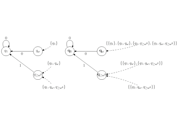
Figure 1. Ordinal automata accepting ${\rm L}_{0}$

2.3. Translation from ${\rm LTL}({\sf U},{\sf S})$ formulae to simple ordinal automata

As usual, a set $Y$ is a maximally Boolean consistent subset of $sub(\phi)$ when the following conditions are satisfied:

1. for every $\psi\in sub(\phi)$, $\neg\psi\in Y$ iff $\psi\not\in Y$,

2. for every $\psi_{1}\wedge\psi_{2}\in sub(\phi)$, $\psi_{1}\wedge\psi_{2}\in Y$ iff $\psi_{1},\psi_{2}\in Y$.

Given a formula $\phi$, the simple ordinal automaton ${\mathcal{A}}_{\phi}=\langle B,Q,I,F,\mathcal{F},\delta_{next},\delta_{lim}\rangle$ is defined as follows:

1. $B=sub(\phi)$.

2. $Q$ is the set of maximally Boolean consistent subsets of $sub(\phi)$.

3. $I$ is the set of locations that contain $\phi$ and no elements of the form $\psi_{1}{\sf S}\psi_{2}$.

4. $F$ is the set of locations with no elements of the form $\psi_{1}{\sf U}\psi_{2}$.

5. A subset $Y$ of $B$ is in $\mathcal{F}$ if there are no $\psi_{1}$ and $\psi_{2}$ such that $\{\psi_{1},\neg\psi_{2},\psi_{1}{\sf U}\psi_{2}\}\subseteq Y$.

6. For all $q,q^{\prime}\in Q$, $\langle q,q^{\prime}\rangle\in\delta_{next}$ $\stackrel{{\scriptstyle\mbox{\tiny def}}}{{\;\Leftrightarrow\;}}$ the conditions below are satisfied:

   1. (next_U): for every $\psi_{1}{\sf U}\psi_{2}\in sub(\phi)$, $\psi_{1}{\sf U}\psi_{2}\in q$ iff either $\psi_{2}\in q^{\prime}$ or $\psi_{1},\psi_{1}{\sf U}\psi_{2}\in q^{\prime}$,

   2. (next_S): for every $\psi_{1}{\sf S}\psi_{2}\in sub(\phi)$, $\psi_{1}{\sf S}\psi_{2}\in q^{\prime}$ iff either $\psi_{2}\in q$ or $\psi_{1},\psi_{1}{\sf S}\psi_{2}\in q$.

7. For all $Y\subseteq B$ and $q\in Q$, $\langle Y,q\rangle\in\delta_{lim}$ $\stackrel{{\scriptstyle\mbox{\tiny def}}}{{\;\Leftrightarrow\;}}$ the conditions below are satisfied:

   1. (lim_U1): if $\psi_{1},\neg\psi_{2},\psi_{1}{\sf U}\psi_{2}\in Y$, then either $\psi_{2}\in q$ or $\psi_{1},\psi_{1}{\sf U}\psi_{2}\in q$,

   2. (lim_U2): if $\psi_{1},\psi_{1}{\sf U}\psi_{2}\in q$ and $\psi_{1}\in Y$, then $\psi_{1}{\sf U}\psi_{2}\in Y$,

   3. (lim_U3): if $\psi_{1}\in Y$, $\psi_{2}\in q$ and $\psi_{1}{\sf U}\psi_{2}$ is in the basis $B$, then $\psi_{1}{\sf U}\psi_{2}\in Y$,

   4. (lim_S): for every $\psi_{1}{\sf S}\psi_{2}\in sub(\phi)$, $\psi_{1}{\sf S}\psi_{2}\in q$ iff ($\psi_{1}\in Y$ and $\psi_{1}{\sf S}\psi_{2}\in Y$).

Even though the conditions above are compatible with the intuition that a location contains the formulae that are promised to be satisfied, at the current stage it might sound mysterious how the conditions have been made up (mainly for the conditions related to limit transitions). For some of them, their justification comes with the proof of Lemma 5.

Let $\sigma$ be an $\alpha$-model and $\phi$ be a formula in ${\rm LTL}({\sf U},{\sf S})$. The Hintikka sequence for $\sigma$ and $\phi$ is an $\alpha$-sequence $H^{\sigma,\phi}$ defined as follows: for every $\beta<\alpha$,

$$H^{\sigma,\phi}(\beta)\stackrel{{\scriptstyle\mbox{\tiny def}}}{{=}}\{\psi\in sub(\phi)~{}:~{}\sigma,\beta\models\psi\}.$$

Given a run $r:\alpha\rightarrow Q$, we write $mod(r):\alpha\rightarrow\mathcal{P}({{\rm PROP}})$ to denote the $\alpha$-model $\sigma$ defined as follows: $\sigma(\beta)\stackrel{{\scriptstyle\mbox{\tiny def}}}{{=}}\{p\in{\rm PROP}:p\in r(\beta)\}$. It is clear that if $r$ is an Hintikka sequence for $\sigma$ and $\phi$, then $mod(r)=\sigma$.

Now we can state the correctness lemma.

Lemma 5.

1. If $\sigma,0\models\phi$, then the Hintikka sequence for $\sigma$ and $\phi$ is an accepting run of ${\mathcal{A}}_{\phi}$.

2. If $r$ is an accepting run of ${\mathcal{A}}_{\phi}$, then $mod(r),0\models\phi$ and $r$ is the Hintikka sequence for $mod(r)$ and $\phi$.

3. $\phi$ is satisfiable iff ${\mathcal{A}}_{\phi}$ has an accepting run.

Proof 2.2.

First, (III) is an immediate consequence of (I) and (II).

1. Suppose that there is a model $\sigma:\alpha\rightarrow\mathcal{P}({{\rm PROP}})$ (with $\alpha>0$) such that $\sigma,0\models\phi$. By using ${\rm LTL}({\sf U},{\sf S})$ semantics, it is straightforward to check that $H^{\sigma,\phi}$ is accepted by ${\mathcal{A}}_{\phi}$.

2. Let $r:\alpha\rightarrow Q$ be an accepting run of ${\mathcal{A}}_{\phi}$. Let us show by structural induction that for all $\psi\in sub(\phi)$ and $\beta<\alpha$, we have $mod(r),\beta\models\psi$ iff $\psi\in r(\beta)$. The base case and the cases with Boolean operators in the induction step are by an easy verification. The only interesting cases in the induction step are related to the temporal operators ${\sf U}$ and ${\sf S}$. Below, let $\sigma$ be $mod(r)$.

   Case ${\sf U}$: $\psi=\psi_{1}{\sf U}\psi_{2}$.
   Let us reason ad absurdum. Suppose that $\{\beta:\psi\in r(\beta)\}\neq\{\beta:\sigma,\beta\models\psi\}$. Let $\beta$ be the smallest ordinal which belongs to only one of these sets. We consider two cases: ($\sigma,\beta\models\psi$ and $\psi\not\in r(\beta)$) – Case I below – or ($\psi\in r(\beta)$ and $\sigma,\beta\not\models\psi$) – Case II below.

   1. Case I: Let $\gamma$ be the smallest ordinal verifying $\beta<\gamma<\alpha$, $\sigma,\gamma\models\psi_{2}$ and for every $\gamma^{\prime}\in(\beta,\gamma)$, we have $\sigma,\gamma^{\prime}\models\psi_{1}\wedge\neg\psi_{2}$. By induction hypothesis, $\psi_{2}\in r(\gamma)$ and for every $\gamma^{\prime}\in(\beta,\gamma)$, $\{\psi_{1},\neg\psi_{2}\}\subseteq r(\gamma^{\prime})$.

      First, we are going to show that $\neg\psi\in r(\gamma^{\prime})$ for every $\gamma^{\prime}\in[\beta,\gamma)$. This is true for $\beta$. Assume that this is true for $\beta^{\prime}$ then it is true for $\beta^{\prime}+1$ by condition (next_U). Assume that $\gamma^{\prime}$ is a limit ordinal and $\psi\not\in r(\beta^{\prime})$ for every $\beta^{\prime}\in[\beta,\gamma^{\prime})$. Then, by condition (lim_U2) we obtain that $\neg\psi\in r(\gamma^{\prime})$. Next, consider two cases:

      Case a): $\gamma$ is a successor, say $\gamma=\beta^{\prime}+1$. We have $\neg\psi\in r(\beta^{\prime})$ and $\psi_{2}\in r(\gamma)$. This contradicts condition (next_U).

      Case b): $\gamma$ is a limit ordinal. In this case $\{\neg\psi,\psi_{1}\}\subseteq B_{lim}(r,\gamma)$ and $\psi_{2}\in r(\gamma)$. This contradicts condition (lim_U3).
      

   2. Case II: Now suppose that $\psi_{1}{\sf U}\psi_{2}\in r(\beta)$ and $\sigma,\beta\not\models\psi_{1}{\sf U}\psi_{2}$.

      Case a): For every $\gamma$ such that $\gamma\in(\beta,\alpha)$, we have $\sigma,\gamma\not\models\psi_{2}$ ($\psi_{2}$ does not hold on $\sigma$ strictly after $\beta$).

      By induction hypothesis, for every $\gamma\in(\beta,\alpha)$, $\neg\psi_{2}\in r(\gamma)$. Let us show that for every $\gamma\in(\beta,\alpha)$, $\{\psi_{1},\psi_{1}{\sf U}\psi_{2}\}\subseteq r(\gamma)$.

      Base case: $\gamma=\beta+1$.
      By condition (next_U), $\psi_{1}{\sf U}\psi_{2}\in r(\beta)$ and $\neg\psi_{2}\in r(\beta+1)$ imply $\{\psi_{1},\psi_{1}{\sf U}\psi_{2}\}\subseteq r(\beta+1)$.

      Induction step:

      1. if $\gamma=\gamma^{\prime}+1$, then by condition (next_U), $\psi_{1}{\sf U}\psi_{2}\in r(\gamma^{\prime})$ and $\neg\psi_{2}\in r(\gamma^{\prime}+1)$ imply $\{\psi_{1},\psi_{1}{\sf U}\psi_{2}\}\subseteq r(\gamma^{\prime}+1)$.

      2. if $\gamma$ is a limit ordinal, by induction hypothesis, $\{\psi_{1},\neg\psi_{2},\psi_{1}{\sf U}\psi_{2}\}\subseteq B_{lim}(r,\gamma)$. By condition (lim_U1), $\{\psi_{1},\psi_{1}{\sf U}\psi_{2}\}\subseteq r(\gamma)$ since $\psi_{2}\not\in r(\gamma)$.

      Consequently, if $\alpha$ is a limit ordinal, then $\{\psi_{1},\neg\psi_{2},\psi_{1}{\sf U}\psi_{2}\}\subseteq B_{lim}(r,\alpha)$ which is in contradiction with the definition of $\mathcal{F}$ in ${\mathcal{A}}_{\phi}$. Similarly, if $\alpha=\alpha^{\prime}+1$, then $\psi_{1}{\sf U}\psi_{2}\in r(\alpha^{\prime})$ which is in contradiction with the definition of $F$.

      Case b): There is a minimal ordinal $\gamma\in(\beta,\alpha)$ such that $\sigma,\gamma\models\neg\psi_{1}\wedge\neg\psi_{2}$ and for every $\gamma^{\prime}\in(\beta,\gamma)$, we have $\sigma,\gamma^{\prime}\models\psi_{1}\wedge\neg\psi_{2}$. By induction hypothesis, $\{\neg\psi_{1},\neg\psi_{2}\}\subseteq r(\gamma)$ and for every $\gamma^{\prime}\in(\beta,\gamma)$, $\{\psi_{1},\neg\psi_{2}\}\subseteq r(\gamma^{\prime})$. Let us show that for every $\gamma^{\prime}\in(\beta,\gamma)$, $\{\psi_{1},\psi_{1}{\sf U}\psi_{2}\}\subseteq r(\gamma^{\prime})$.

      Base case: $\gamma^{\prime}=\beta+1$.
      By condition (next_U), $\psi_{1}{\sf U}\psi_{2}\in r(\beta)$ and $\neg\psi_{2}\in r(\beta+1)$ imply $\{\psi_{1},\psi_{1}{\sf U}\psi_{2}\}\subseteq r(\gamma^{\prime})$.

      Induction step:

      1. If $\gamma^{\prime}=\gamma^{\prime\prime}+1$, then by condition (next_U), $\psi_{1}{\sf U}\psi_{2}\in r(\gamma^{\prime\prime})$ and $\neg\psi_{2}\in r(\gamma^{\prime\prime}+1)$ imply $\{\psi_{1},\psi_{1}{\sf U}\psi_{2}\}\subseteq r(\gamma^{\prime\prime}+1)$.

      2. If $\gamma^{\prime}$ is a limit ordinal, then by induction hypothesis, $\{\psi_{1},\neg\psi_{2},\psi_{1}{\sf U}\psi_{2}\}\subseteq B_{lim}(r,\gamma^{\prime})$. By condition (lim_U1), $\{\psi_{1},\psi_{1}{\sf U}\psi_{2}\}\subseteq r(\gamma^{\prime})$ since $\psi_{2}\not\in r(\gamma^{\prime})$.

      Consequently, if $\gamma$ is a limit ordinal, then $\{\psi_{1},\neg\psi_{2},\psi_{1}{\sf U}\psi_{2}\}\subseteq B_{lim}(r,\gamma)$ which leads to a contradiction by condition (lim_U1). Indeed, by induction hypothesis, $\{\neg\psi_{1},\neg\psi_{2}\}\subseteq r(\gamma)$. Similarly, if $\gamma=\gamma^{\prime}+1$, then $\psi_{1}{\sf U}\psi_{2}\not\in r(\gamma^{\prime})$ which leads to a contradiction by condition (next_U).
      

   Case ${\sf S}$: $\psi=\psi_{1}{\sf S}\psi_{2}$.
   Let us reason ad absurdum. Suppose that $\{\beta:\psi\in r(\beta)\}\neq\{\beta:\sigma,\beta\models\psi\}$. Let $\beta$ be the smallest ordinal that belongs to only one of these sets. Again, we distinguish two cases, namely either ($\sigma,\beta\models\psi$ and $\psi\not\in r(\beta)$) – Case I below – or ($\psi\in r(\beta)$ and $\sigma,\beta\not\models\psi$) – Case II below.

   1. Case I: So $\beta>0$ and there is $\gamma\in[0,\beta)$ such that $\sigma,\gamma\models\psi_{2}$ and for every $\gamma^{\prime}\in(\gamma,\beta)$, we have $\sigma,\gamma^{\prime}\models\psi_{1}$. By induction hypothesis, $\psi_{2}\in r(\gamma)$ and for every $\gamma^{\prime}\in(\gamma,\beta)$, $\psi_{1}\in r(\gamma^{\prime})$. Observe that for every $\gamma^{\prime}\in(\gamma,\beta)$, we have $\sigma,\gamma^{\prime}\models\psi$ and $\psi\in r(\gamma^{\prime})$ ($\beta$ is minimal).

      1. If $\beta=\beta^{\prime}+1$ then by condition (next_S) $\psi_{2}\not\in r(\beta^{\prime})$ and $\{\psi_{1},\psi_{1}{\sf S}\psi_{2}\}\not\subseteq r(\beta^{\prime})$. If $\gamma=\beta^{\prime}$, then this leads to a contradiction since $\psi_{2}\in r(\gamma)$. Similarly, if $\gamma<\beta^{\prime}$, then $\psi\not\in r(\beta^{\prime})$ since $\psi_{1}\in r(\beta^{\prime})$. Since $\sigma,\beta^{\prime}\models\psi_{1}{\sf S}\psi_{2}$, this leads to a contradiction by the minimality of $\beta$.

      2. If $\beta$ is a limit ordinal, then by condition (lim_S) either $\psi_{1}\not\in B_{lim}(r,\beta)$ or $\psi_{1}{\sf S}\psi_{2}\not\in B_{lim}(r,\beta)$. By induction hypothesis, $\psi_{1}\in B_{lim}(r,\beta)$. Hence, there is $\beta^{\prime}\in(\gamma,\beta)$ such that $\psi_{1}{\sf S}\psi_{2}\not\in r(\beta^{\prime})$, which is in contradiction with the minimality of $\beta$.

   2. Case II:

      Case a): For every $\gamma\in[0,\beta)$, $\sigma,\beta\not\models\psi_{2}$.
      By induction hypothesis, for every $\gamma\in[0,\beta)$, $\psi_{2}\not\in r(\gamma)$. Moreover, for every $\gamma\in[0,\beta)$, we have $\sigma,\beta\not\models\psi_{1}{\sf S}\psi_{2}$.

      1. If $\beta=\beta^{\prime}+1$ then by condition (next_S), $\{\psi_{1},\psi_{1}{\sf S}\psi_{2}\}\subseteq r(\beta^{\prime})$ which leads to a contradiction by minimality of $\beta$.

      2. If $\beta$ is a limit ordinal, then $\{\psi_{1},\psi_{1}{\sf S}\psi_{2}\}\subseteq B_{lim}(r,\beta)$ by condition (lim_S). Hence, for some $\beta^{\prime}<\beta$, $\psi_{1}{\sf S}\psi_{2}\in r(\beta^{\prime})$, which leads again to a contradiction by the minimality of $\beta$.

      3. If $\beta=0$, then we also have a contradiction since $r(0)$ does not contain any since formulae. Observe that in the previous case analyses with ordinals, the case “0” has been irrelevant.

      Case b): $\sigma,\beta\not\models\psi$ and not a).
      Remember that $\psi\in r(\beta)$. There is $\beta^{\prime}<\beta$ such that $\sigma,\beta^{\prime}\not\models\psi_{1}$. Otherwise, by induction hypothesis and by not a), we have $\sigma,\beta\models\psi$, a contradiction.
      Case b.1: There is a maximal position $\gamma<\beta$ such that $\sigma,\gamma\not\models\psi_{1}$.
      For every $\gamma^{\prime}\in(\gamma,\beta)$, we have $\sigma,\gamma\not\models\psi_{2}$, otherwise $\sigma,\beta\models\psi$ which would lead to a contradiction. Let us show by transfinite induction that for every $\gamma^{\prime}\in(\gamma,\beta]$, $\psi\not\in r(\gamma^{\prime})$.

      Base case: $\gamma^{\prime}=\gamma+1$.
      $\neg\psi_{1},\neg\psi_{2}\in r(\gamma)$ imply by condition (next_S) that $\psi\not\in r(\gamma^{\prime})$.

      Induction step:

      1. If $\gamma^{\prime}=\gamma^{\prime\prime}+1$, then $\neg\psi_{2},\neg\psi\in r(\gamma^{\prime\prime})$ by induction hypothesis. By condition (next_S) $\psi\not\in r(\gamma^{\prime})$.

      2. If $\gamma^{\prime}$ is a limit ordinal, then $\neg\psi\in B_{lim}(r,\gamma^{\prime})$ and by condition (lim_S), $\psi\not\in r(\gamma^{\prime})$.

      Hence, $\psi\not\in r(\beta)$, which leads to a contradiction.

      Case b.2 There is no maximal position $\gamma<\beta$ such that $\sigma,\gamma\not\models\psi_{1}$ (the most delicate case).
      Consequently, there is a unique position $\gamma\leq\beta$ such that for every $\gamma^{\prime}<\gamma$, there is $\gamma^{\prime}<\gamma^{\prime\prime}<\gamma$ verifying $\neg\psi_{1}\in r(\gamma^{\prime\prime})$. This means that

      1. for every $\gamma^{\prime}\in[\gamma,\beta]$, $\psi_{1}\in r(\gamma^{\prime})$,

      2. $\psi_{1}\not\in B_{lim}(r,\gamma)$ and,

      3. by condition (lim_S) $\psi\not\in r(\gamma)$.

      Moreover, for every $\gamma^{\prime}\in(\gamma,\beta)$, $\neg\psi_{2}\in r(\gamma^{\prime})$ otherwise by induction hypothesis, $\sigma,\beta\models\psi$, which would lead to a contradiction. Let us show by transfinite induction that for every $\gamma^{\prime}\in(\gamma,\beta]$, $\psi\not\in r(\gamma^{\prime})$.

      Base case: $\gamma^{\prime}=\gamma+1$.
      $\neg\psi,\neg\psi_{2}\in r(\gamma)$ imply by condition (next_S) $\psi\not\in r(\gamma^{\prime})$.

      Induction step:

      1. If $\gamma^{\prime}=\gamma^{\prime\prime}+1$, then $\neg\psi_{2},\neg\psi\in r(\gamma^{\prime\prime})$ by induction hypothesis. By condition (next_S) $\psi\not\in r(\gamma^{\prime})$.

      2. If $\gamma^{\prime}$ is a limit ordinal, then $\neg\psi\in B_{lim}(r,\gamma^{\prime})$ and by condition (lim_S), $\psi\not\in r(\gamma^{\prime})$.

      Hence, $\psi\not\in r(\beta)$, which leads to a contradiction.∎

3. Short Run Properties

In this section, we establish pumping arguments that are useful to show that

1. in order to check the satisfiability status of the formula $\phi$, there is no need to consider models of length greater than $\omega^{|\phi|+2}$,

2. simple ordinal automata cannot distinguish ordinals with identical tails (defined below precisely with the notion of truncation).

Let ${\mathcal{A}}$ be a simple ordinal automaton and $Y$ be a subset of its basis. $Y$ is said to be present in ${\mathcal{A}}$ iff either there is a limit transition of the form $\langle Y,q\rangle$ in ${\mathcal{A}}$ or $Y\in\mathcal{F}$. Given a set $Y$ present in ${\mathcal{A}}$, its weight, noted ${\rm weight}(Y)$, is the maximal $l$ such that $Y_{1}\subset Y_{2}\subset\cdots\subset Y_{l}$ is a sequence of present subsets in ${\mathcal{A}}$ and $Y_{1}=Y$ ($\subset$ denotes proper subset inclusion). Obviously, ${\rm weight}(Y)\leq{\rm card}(B)+1$.

Given a path $r:\alpha\rightarrow Q$ in ${\mathcal{A}}$ with a limit ordinal $\alpha\geq\omega$, its weight, noted ${\rm weight}(r)$, is the maximal value in the set

$$\{{\rm weight}(B_{lim}(r,\beta)):\beta<\alpha,\ \beta\ {\rm is\ a\ limit\ ordinal}\}\cup\{{\rm weight}(B_{lim}(r))\}$$

When $\alpha$ is a successor ordinal, the maximal value is computed only from the first set of the above union. By convention, if a path has no limit transition, then its weight is zero (equivalently, its length is strictly less than $\omega+1$). Furthermore, we write ${\rm all}(r)$ to denote the set

$${\rm all}(r)\stackrel{{\scriptstyle\mbox{\tiny def}}}{{=}}\bigcap_{\beta<\alpha}r(\beta)$$

that corresponds to the set of elements from the basis that are present in all locations of the run $r$. Let $r$, $r^{\prime}$ be two paths of respective length $\alpha$ and $\alpha^{\prime}$. We say that $r$ and $r^{\prime}$ are congruent, written $r\sim r^{\prime}$, iff the conditions below are meet:

1. $r(0)=r^{\prime}(0)$.

2. Either both $\alpha$ and $\alpha^{\prime}$ are successor ordinals and $r(\alpha-1)=r^{\prime}(\alpha^{\prime}-1)$ or both $\alpha$ and $\alpha^{\prime}$ are limit ordinals and $B_{lim}(r)=B_{lim}(r^{\prime})$.

3. ${\rm all}(r)={\rm all}(r^{\prime})$.

Let $r_{1}$ be a path of length $\alpha$ and $r_{2}$ be a path of length $\beta$ such that if $\alpha$ is a limit ordinal then $\langle B_{lim}(r_{1}),r_{2}(0)\rangle\in\delta_{lim}$ otherwise $r_{1}(\alpha-1)=r_{2}(0)$. The concatenation $r_{1}\cdot r_{2}$ is the path $r$ of length $\alpha+\beta$ such that for $\gamma\in[0,\alpha)$, $r(\gamma)=r_{1}(\gamma)$ and for $\gamma\in[0,\beta)$, $r(\alpha+\gamma)=r_{2}(\gamma)$. For every ordinal $\alpha$, the concatenation of $\alpha$-sequences of paths is defined similarly. The relation $\sim$ is a congruence for the concatenation operation on paths as stated in details below.

Lemma 6.

1. Let $r\cdot r_{0}\cdot r^{\prime}$ and $r_{1}$ be two paths such that $r_{0}\sim r_{1}$. Then, $r\cdot r_{1}\cdot r^{\prime}$ is a path that is congruent to $r\cdot r_{0}\cdot r^{\prime}$.

2. Let $r_{0}^{0},r_{0}^{1},r_{0}^{2},\ldots$ and $r_{1}^{0},r_{1}^{1},r_{1}^{2},\ldots$ be two $\omega$-sequences of pairwise consecutive paths such that for $i\geq 0$, $r_{0}^{i}\sim r_{1}^{i}$ and their length is a successor ordinal. If $r\cdot(r_{0}^{0}\cdot r_{0}^{1}\cdot r_{0}^{2}\cdot\ldots)\cdot r^{\prime}$ is a path, then it is congruent to $r\cdot(r_{1}^{0}\cdot r_{1}^{1}\cdot r_{1}^{2}\cdot\ldots)\cdot r^{\prime}$.

The proof of the above lemma is by an easy verification but observe that for the proof of (II) the third set of equalities from the definition of the congruence $\sim$ ensures that $r\cdot(r_{0}^{0}\cdot r_{0}^{1}\cdot r_{0}^{2}\cdot\ldots)\cdot r^{\prime}$ is a path.

Lemma 7.

Let $r:\alpha\rightarrow Q$ be a path in ${\mathcal{A}}$ for some countable ordinal $\alpha$ such that if $\alpha$ is a limit ordinal, then $B_{lim}(r)$ is present in ${\mathcal{A}}$. Then, there is a path $r^{\prime}:\alpha^{\prime}\rightarrow Q$ for $\alpha^{\prime}<\omega^{max(1,{\rm weight}(r))+1}$ such that $r\sim r^{\prime}$ and ${\rm weight}(r^{\prime})\leq{\rm weight}(r)$.