Confirmation of a Retrograde Orbit for Exoplanet WASP-17b

Abstract

We present high-precision radial velocity observations of WASP-17 throughout the transit of its close-in giant planet, using the MIKE spectrograph on the 6.5m Magellan Telescope at Las Campanas Observatory. By modeling the Rossiter-McLaughlin effect, we find the sky-projected spin-orbit angle to be $\lambda=167.4\pm 11.2$ deg. This independently confirms the previous finding that WASP-17b is on a retrograde orbit, suggesting it underwent migration via a mechanism other than just the gravitational interaction between the planet and the disk. Interestingly, our result for $\lambda$ differs by $45\pm 13$ deg from the previously announced value, and we also find that the spectroscopic transit occurs $15\pm 5$ min earlier than expected, based on the published ephemeris. The discrepancy in the ephemeris highlights the need for contemporaneous spectroscopic and photometric transit observations whenever possible.

1. Introduction

Knowledge of the angle $\psi$ between a star’s spin vector and a planet’s orbital angular momentum vector contains information about the planetary formation process. This is especially so for Hot Jupiters, which are thought to have “migrated” inward from large orbital distances (Lin et al., 1996). One possible migration mechanism involves the gravitational interaction between the planet and the gas in the protoplanetary disk (e.g. Lin et al., 1996; Ida & Lin, 2004). Such interactions would preserve a prograde orbit, and could not account for Hot Jupiters with retrograde orbits ($\psi>90^{\circ}$) unless the protoplanetary disk was initially misaligned with the star (Bate et al., 2010). Other migration mechanisms, involving planet-planet scattering and Kozai cycles, (e.g. Nagasawa et al., 2008) can produce retrograde orbits. Therefore by measuring $\psi$ one gains insight into the migration history of a particular planetary system.

The Rossiter-McLaughlin effect (Rossiter, 1924; McLaughlin, 1924) occurs when part of the rotating stellar photosphere is eclipsed by a companion star or planet. This removes a velocity component of the observed rotationally- broadened line profiles, causing a pattern of anomalous radial velocities to be observed throughout the eclipse. Although this effect does not reveal $\psi$, it does give a measure of $\lambda$, the angle between the sky projection of the stellar spin vector and the planetary orbital angular momentum. The Rossiter-McLaughlin effect has now been used to measure $\lambda$ for 28 transiting planet systems (see Triaud et al. (2010) or Winn et al. (2010)).

The transiting Hot Jupiter WASP-17b, which was discovered by Anderson et al. (2010), is reported to have a planetary radius of $R_{P}=1.74~{}R_{J}$ and a host star rotational velocity of $v\sin i=9$km s^-1. The deep transit and fast stellar rotation make it a propitious target for Rossiter-McLaughlin effect observations.

Anderson et al. (2010) reported that the planet appeared to be in a retrograde orbit, based on three radial-velocity measurements that were obtained during transits. Subsequently, the same group announced further radial velocity measurements of WASP-17, with denser time sampling (Triaud et al., 2010). Those data gave much stronger support to the claim of a retrograde orbit, and indeed gave a value for $\lambda$ nearly identical to the value derived by Anderson et al. (2010). In this Letter we present new observations and an independent confirmation of the likely retrograde orbit of the WASP-17 system, though with a significantly different derived value for $\lambda$.

2. Observations

On the night of 2010 May 11, we obtained high-resolution spectra of WASP-17 using the Magellan Inamori Kyocera Echelle (MIKE) spectrograph on the 6.5m Magellan II (Clay) telescope at Las Campanas Observatory. MIKE was used in its standard configuration with a 0.35″ slit and fast readout mode, which delivered 32 red echelle orders with wavelengths from 5000-9500 Å and with a resolving power of $R\approx 48,000$. Spectra were taken continuously for 9 hours, with an interruption of approximately 30 minutes when the star crossed the meridian near the zenith. A total of 33 spectra of WASP-17 were obtained, with 600 s exposures. ThAr calibration frames bracketed each spectrum. Observing conditions were good, although some high, thin clouds were present in the latter half of the night. The moon was down throughout the WASP-17 observations, and the seeing was 0.5-0.7″.

The spectra were reduced using the Carnegie MIKE pipeline developed by Dan Kelson. Radial velocities were determined via cross correlation with respect to a template spectrum. We tested different choices for the template spectrum, including a radial velocity standard observed on the same night and various individual WASP-17 spectra. The lowest inter-order scatter was obtained when using the highest signal-to-noise WASP-17 spectrum as the template. This spectrum was also obtained at low airmass (1.005). For the cross-correlation analysis we selected 13 echelle orders that were free of obvious telluric lines and had a signal-to-noise ratio exceeding 100 pixel^-1. Cross-correlation was performed using the IRAF task $fxcor$. We used the O₂ absorption features from 6870-6900 Å to provide a constant reference for our wavelength solutions for each spectrum. These absorption bands have been shown to be stable at the 5 m s^-1 level over short timescales (Figueira et al., 2010).

MIKE lacks an atmospheric dispersion corrector, and this resulted in an airmass-dependent systematic trend in the radial velocity measurements, with an amplitude that increased for bluer echelle orders. The continuous nine-hour monitoring allowed us to track this systematic trend and account for it during the model-fitting procedure, as described in Section 3. The order-averaged, airmass-corrected radial velocities are given in Table 1, with uncertainties taken to be the standard deviation of the mean of the results of all 13 orders.

3. Analysis

Our model for the radial velocity data has the form:

$$V_{{\rm calc},n}(t)=V_{\rm orb}(t)+V_{\rm RM}(t)+c_{0}+c_{1}n+(c_{2}+c_{3}n)X,$$ (1)

where $V_{{\rm calc},n}(t)$ is the calculated radial velocity at time $t$ in echelle order $n$ (ranging from 1 to 13), $V_{\rm orb}$ is the radial velocity due to the star’s orbital motion (assumed to be circular), $V_{\rm RM}$ is the transit-specific “anomalous velocity” due to the Rossiter-McLaughlin effect, and $\{c_{0},c_{1},c_{2},c_{3}\}$ are constants specifying the offset between the relative barycentric velocity of WASP-17 and the arbitrary template spectrum that was used to calculate radial velocities. To account for the wavelength-dependent airmass trend mentioned in the previous section, the offset was allowed to be a linear function of both order number $n$ (effectively a wavelength index) and airmass $X$.

Many approaches have been taken to model the Rossiter-McLaughlin effect, such as the pixellated photospheric model of Queloz et al. (2000), the first-moment approach of Ohta et al. (2005) and Giménez (2006), the forward-modeling approach of Winn et al. (2005) or the spectral line fitting of Albrecht et al. (2009) and Collier Cameron et al. (2010). In our case the most applicable and convenient model is the analytic formula of Hirano et al. (2010),

$$V_{\rm RM}(t)=-\delta(t)~{}v_{p}(t)\left[\frac{2v_{0}^{2}+2(v\sin i)^{2}}{2v_{0}^{2}+(v\sin i)^{2}}\right]^{3/2}$$

$$\left[1-\frac{v_{p}(t)^{2}}{2v_{0}^{2}+(v\sin i)^{2}}\right],$$ (2)

where $\delta(t)$ is the loss of light during the transit, $v_{p}(t)$ is the mean radial velocity of the small portion of the photosphere that is hidden by the planet, $v\sin i$ is the stellar projected rotation rate, and $v_{0}$ is the velocity width of the spectral lines that would be seen from a small portion of the photosphere (i.e. due to mechanisms other than rotation). This formula relates the phase of the transit to the radial velocity anomaly derived from cross-correlation.

To calculate $v_{p}(t)$ we assumed that the stellar photosphere rotates uniformly with an angle $\lambda$ between the sky projections of the spin vector and the orbital angular momentum vector (see, e.g., Ohta et al. (2005) or Gaudi & Winn (2007)). We took $v\sin i$ to be a free parameter, and $v_{0}$ was constrained by the condition that the quadrature sum of $v_{0}$ and $v\sin i$ should equal the observed total linewidth of 11 km s^-1 (Anderson et al., 2010).

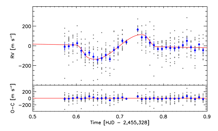
Figure 1.— The spectroscopic transit of WASP-17b. Top.—Radial velocity variation observed on the night of 2010 May 11-12, along with the best-fitting model. The small gray points are the order-by-order radial velocities that were fitted. The larger blue points are averages of the results from all orders. Bottom.—Residuals between the data and the best-fitting model.

To calculate $\delta(t)$, we assumed a linear limb-darkening law with a fixed coefficient of 0.7, and used the analytic formulas of Mandel & Agol (2002), as implemented by Pál (2008). The parameters of the photometric model were the planet-to-star radius ratio $R_{p}/R_{\star}$, orbital inclination $i$, and normalized stellar radius $R_{\star}/a$ (where $a$ is the orbital distance). Some of the transit characteristics are more tightly constrained by previous observations of photometric transits than by the radial velocity data presented here. Hence, we used Gaussian priors for the transit depth $(R_{p}/R_{\star})^{2}$, total duration $t_{\rm IV}-t_{\rm I}$, partial duration $t_{\rm IV}-t_{\rm III}$, orbital period $P$, and time of transit $T_{c}$, based on the results presented by Anderson et al. (2010) (see their Table 4, case 3). We also used those results to set a Gaussian prior for $K$, the orbital velocity semi-amplitude, since our coverage of the spectroscopic orbit is sparse.

All together there are 11 adjustable parameters in our model fit, of which 7 are mainly determined by our new radial velocity data: $\lambda$, $v\sin i$, $c_{0}$, $c_{1}$, $c_{2}$, $c_{3}$, and the time of conjunction $T_{c}$. The other 4 parameters, $R_{p}/R_{\star}$, $i$, $R_{\star}/a$, and $K$, are controlled mainly by the priors. We determined the best-fitting parameter values and their 68.3% confidence limits with a Monte Carlo Markov Chain (MCMC) algorithm that we have described elsewhere (see, e.g., Winn et al. (2007)). The likelihood was taken to be $\exp(-\chi^{2}/2)$ with

$$\chi^{2}=\sum_{i=1}^{33}\sum_{n=1}^{13}\left[\frac{v_{\rm obs}(t_{i},n)-v_{\rm calc}(t_{i},n)}{\sigma}\right]^{2},$$ (3)

where $v_{\rm obs}(t_{i},n)$ is the radial velocity measured at time $t_{i}$ in echelle order $n$, and $v_{\rm calc}(t_{i},n)$ are the calculated radial velocities. We found that the choice $\sigma=92$ m s^-1 gave $\chi^{2}=N_{\rm dof}$ for the best-fitting model, and is also approximately equal to the scatter observed in the residuals to the best-fitting model, so we used this value in the MCMC analysis.

Table 2 gives the resulting best-fit parameter values. Figure 1 shows the airmass-corrected radial velocities as a function of time, along with the best-fitting model and the residuals. Figure 2 illustrates the airmass correction for three separate echelle orders. Figure 3 displays the marginalized, joint a posteriori probability distributions involving $\lambda$ and the other model parameters.

Figure 2.— Illustration of airmass correction. The radial velocities for echelle orders 61, 59, and 57 (from top to bottom), along with the best-fitting model that includes both an airmass correction and the Rossiter-McLaughlin effect. Central wavelengths of the orders are indicated on the plot. The lower panel shows the time dependence of the airmass.

The radial velocity data clearly exhibit an “upside-down” Rossiter-McLaughlin effect: an anomalous blueshift for the first half of the transit, followed by an anomalous redshift for the second half. Our result for the projected stellar rotation velocity, $v\sin i_{\star}=8.61\pm 0.45$ km s^-1, is in agreement with the results of Anderson et al. (2010) and Triaud et al. (2010). However, our finding of $\lambda=167.4\pm 11.2$ deg does not agree with either of the previously reported results. Anderson et al. (2010) found $\lambda=210.7^{+11.5}_{-8.9}$ deg, although this result was based on only 3 data points. More significant is the result by Triaud et al. (2010) of $\lambda=212.7^{+5.5}_{-5.9}$ deg, based on two data sets densely sampling the transit. The difference between our result for $\lambda$ and that of Triaud et al. (2010) is $45\pm 13$ deg, or 3.5$\sigma$ away from zero.

We do not know the reason for the discrepancy. We have sparser coverage of the spectroscopic orbit than did Triaud et al. (2010), but this did not bias our results: we used the results of Anderson et al. (2010) to set a prior for $K$, and also found that the results for $K$ and $\lambda$ are uncorrelated. We also checked to see if the gap in our time coverage when WASP-17 was at zenith has biased our results: we fitted fake data with $\lambda=210\fdg 7$ and the same time coverage and velocity errors as our MIKE data, and found $\lambda=206^{\circ}\pm 9^{\circ}$, i.e., the result was not biased. We also fitted the Triaud et al. (2010) data ourselves and found $\lambda=208^{\circ}\pm 12^{\circ}$. Although this reduces the discrepancy in results to 2.5$\sigma$, it indicates that the differences in $\lambda$ values cannot be attributed solely to differences in fitting procedures. An important step in our data analysis was fitting and removing the airmass trend in our radial velocity data. We fitted for the airmass terms simultaneously with the Rossiter-McLaughlin model, and therefore our results do take into account any correlations between the airmass parameters and the other parameters including $\lambda$. However, these errors are internal to the choice of our model, which is linear in airmass and order number. This model seems reasonable and provides a satisfactory fit to the data; however it is impossible to exclude the possibility that the true dependence is more subtle and that this has altered the shape of the Rossiter-McLaughlin effect.

According to the ephemeris of Anderson et al. (2010), the predicted time of conjunction for the event we observed is HJD 2,455,328.6814$~{}\pm 0.0017$, which is earlier by $15\pm 5$ min than the time we measured. Either the transits are nonperiodic, or the uncertainties in at least some of the transit times were underestimated. A straight-line fit to the epochs and transit times in Table 5 of Anderson et al. (2010) gives $\chi^{2}=36$ with 11 degrees of freedom, i.e., statistically different than random. For this reason, it is likely that the true uncertainty in the period is larger than the previously reported uncertainty, by a factor of about $\sqrt{36/11}$ or 1.8.

Consequently, we conclude that our timing offset from the ephemeris of Anderson et al. (2010) is at most a 1.5$\sigma$ discrepancy. The uncertainty in the time of conjunction would be best addressed in the future by obtaining high-quality photometric data simultaneously with spectroscopic observations. However we note that this ephemeris discrepancy cannot account for the difference between our result for $\lambda$ and that of Triaud et al. (2010).

Our result for $\lambda$ is consistent with a retrograde orbit, but it must be remembered that $\lambda$ is a sky-projected quantity. The true angle $\psi$ between the vectors is given by

$$\cos\psi=\cos i_{\star}\cos i+\sin i_{\star}\sin i\cos\lambda,$$ (4)

where $i$ and $i_{\star}$ are the line-of-sight inclinations of the orbital and stellar angular momentum vectors, respectively. Using $i=86.95_{-0.63}^{+0.87}$ deg from Anderson et al. (2010), and supposing $i_{\star}$ to be drawn from an “isotropic” distribution (uniform in $\cos i_{\star}$), we find $\psi>92\fdg 6$ with 99.73% confidence. In this sense, the WASP-17b orbit is very likely to be retrograde ($\psi>90^{\circ}$), although nearly pole-on configurations ($\psi\approx 90^{\circ}$) are possible.

The assumption of an isotropic distribution in $i_{\star}$ neglects our prior knowledge that main-sequence stars have somewhat predictable rotation rates, and therefore that the measured value of $v\sin i_{\star}$ also bears information about $i_{\star}$. Recently, Schlaufman (2010) used this insight to seek evidence for small values of $\sin i_{\star}$ (and therefore large spin-orbit misalignments along the line of sight) among all the transit hosts. He did not identify WASP-17 as one of the systems with a likely small value of $\sin i_{\star}$. In light of this analysis, our observation of a large $\lambda$ favors a more nearly retrograde orbits over polar orbits.

Figure 3.— Results for the model parameters, based on our MCMC analysis of the radial velocity data, for parameters which show a degree of correlation with $\lambda$. The contours represent 68%, 95%, and 99.73% confidence limits. The quantity $\Delta T_{c}$ is defined as $T_{c}$ minus the optimized value of HJD 2,455,328.6918.

4. Discussion

It is now ten years since the first reported detection of the Rossiter-McLaughlin effect due to a transiting planet (Queloz et al., 2000). As with many other properties of extrasolar planets, the Rossiter-McLaughlin effect observations have thrown up surprises, with systems that appear very different from those in our own Solar System. The Hot Jupiter HAT-P-7b was found to be on a polar or retrograde orbit, by independent measurements of Narita et al. (2009) and Winn et al. (2009). Similarly WASP-17b has now been confirmed to be in a retrograde orbit by two independent groups (Triaud et al., 2010, this work). It now seems that at least a fraction of Hot Jupiters are migrating by mechanisms other than disk migration, or that proto-planetary disks are frequently misaligned with their stars.

The work of Fabrycky & Winn (2009) suggested that we may be seeing two different populations of Hot Jupiters that have migrated via different mechanisms. The results of this work adds weight to that suggestion, however a larger statistical sample will be needed before this can be robustly confirmed. Only a larger sample of planets with known $\lambda$ values will allow correlations with parameters such as planetary mass, planetary radius, metallicity, and stellar mass to be robustly tested. Winn et al. (2010) have proposed that misaligned Hot Jupiters occur preferentially around hot stars ($T_{\rm eff}>6250$ K), of which WASP-17 is a supporting example. Fortunately the discovery rate of transiting planets orbiting bright stars is set to rise due to large-scale ground-based surveys such as SuperWASP Cameron et al. (2007) and HAT-South (Bakos et al., 2009), and proposed space-based projects such as TESS (Deming et al., 2009) and PLATO (Catala & PLATO Consortium, 2008).

Table 1WASP-17 Radial Velocities (order averaged)

Time	Radial	Radial velocity
HJD	velocity (m s-1)	uncertainty (m s-1)
$2455328.57331$	$-9.88$	$38.75$
$2455328.58273$	$-4.73$	$32.47$
$2455328.59219$	$9.70$	$27.08$
$2455328.60194$	$26.88$	$27.51$
$2455328.61135$	$-49.67$	$37.43$
$2455328.62035$	$-87.48$	$24.96$
$2455328.62971$	$-68.18$	$20.08$
$2455328.63921$	$-110.63$	$40.87$
$2455328.64876$	$-141.71$	$30.59$
$2455328.65817$	$-124.57$	$35.23$
$2455328.66761$	$-92.68$	$27.30$
$2455328.67700$	$-135.62$	$27.72$
$2455328.68633$	$-42.40$	$34.15$
$2455328.69570$	$-13.34$	$24.05$
$2455328.70557$	$50.30$	$23.05$
$2455328.71481$	$37.16$	$15.00$
$2455328.74077$	$164.59$	$17.62$
$2455328.75012$	$86.38$	$23.37$
$2455328.75939$	$86.77$	$38.93$
$2455328.76863$	$31.27$	$30.88$
$2455328.77785$	$6.61$	$39.38$
$2455328.78711$	$-32.55$	$18.04$
$2455328.79641$	$-30.80$	$24.08$
$2455328.80593$	$-15.31$	$24.74$
$2455328.81546$	$-23.01$	$32.34$
$2455328.82536$	$-25.39$	$32.21$
$2455328.83495$	$-18.66$	$20.94$
$2455328.84430$	$6.76$	$26.41$
$2455328.85358$	$50.02$	$32.97$
$2455328.86289$	$-15.15$	$25.22$
$2455328.87214$	$-45.57$	$30.49$
$2455328.88145$	$13.95$	$15.26$
$2455328.89069$	$-44.50$	$24.20$

Table 2Model Parameters for WASP-17b

Parameter	Value
Parameters determined mainly by the
new radial velocity data
Projected spin-orbit angle, $\lambda$ [deg]	$167.6\pm 11.4$
Projected stellar rotation rate, $v\sin i_{\star}$ [km s-1]	$8.61\pm 0.45$
Radial velocity offset, $c_{0}$ [m s-1]	$-0.267\pm 0.074$
Order dependence of radial velocity offset, $c_{1}$ [m s-1 order-1]	$-0.79\pm 0.11$
Airmass term, $c_{2}$ [m s-1 airmass-1]	$0.233\pm 0.061$
Order dependence of airmass term, $c_{3}$ [m s-1 airmass-1 order-1]	$0.738\pm 0.093$
Parameters determined mainly by priors
Velocity semi-amplitude, $K$ [m s-1]	$55.9\pm 5.0$
Time of conjunction, $T_{c}$ [HJD-2,450,000]	$5,328.6919\pm 0.0027$
Transit depth, $(R_{p}/R_{\star})^{2}$	$0.01676\pm 0.00027$
Total transit duration, $t_{\rm IV}-t_{\rm I}$ [hr]	$4.368\pm 0.037$
Partial transit duration, $t_{\rm IV}-t_{\rm III}$ [hr]	$0.566\pm 0.039$

References

- Albrecht et al. (2009) Albrecht, S., Reffert, S., Snellen, I. A. G., & Winn, J. N. 2009, Nature, 461, 373
- Anderson et al. (2010) Anderson, D. R., et al. 2010, ApJ, 709, 159
- Bakos et al. (2009) Bakos, G., et al. 2009, in IAU Symp. 253, Transiting Planets, ed. F. Pont, D. D. Sasselov, & M. J. Holman (Cambridge: Cambridge Univ. Press), 354
- Bate et al. (2010) Bate, M. R., Lodato, G., & Pringle, J. E. 2010, MNRAS, 401, 1505
- Cameron et al. (2007) Cameron, A. C., et al. 2007, MNRAS, 375, 951
- Catala & PLATO Consortium (2008) Catala, C., & PLATO Consortium. 2008, Journal of Physics Conference Series, 118, 012040
- Collier Cameron et al. (2010) Collier Cameron, A., Bruce, V. A., Miller, G. R. M., Triaud, A. H. M. J., & Queloz, D. 2010, MNRAS, 403, 151
- Deming et al. (2009) Deming, D., et al. 2009, PASP, 121, 952
- Fabrycky & Winn (2009) Fabrycky, D. C., & Winn, J. N. 2009, ApJ, 696, 1230
- Figueira et al. (2010) Figueira, P., Pepe, F., Lovis, C., & Mayor, M. 2010, arXiv1003.0541
- Gaudi & Winn (2007) Gaudi, B. S., & Winn, J. N. 2007, ApJ, 655, 550
- Giménez (2006) Giménez, A. 2006, ApJ, 650, 408
- Hirano et al. (2010) Hirano, T., Suto, Y., Taruya, A., Narita, N., Sato, B., Johnson, J. A., & Winn, J. N. 2010, ApJ, 709, 458
- Ida & Lin (2004) Ida, S., & Lin, D. N. C. 2004, ApJ, 616, 567
- Lin et al. (1996) Lin, D. N. C., Bodenheimer, P., & Richardson, D. C. 1996, Nature, 380, 606
- Mandel & Agol (2002) Mandel, K., & Agol, E. 2002, ApJ, 580, L171
- McLaughlin (1924) McLaughlin, D. B. 1924, ApJ, 60, 22
- Nagasawa et al. (2008) Nagasawa, M., Ida, S., & Bessho, T. 2008, ApJ, 678, 498
- Narita et al. (2009) Narita, N., Sato, B., Hirano, T., & Tamura, M. 2009, PASJ, 61, L35
- Ohta et al. (2005) Ohta, Y., Taruya, A., & Suto, Y. 2005, ApJ, 622, 1118
- Pál (2008) Pál, A. 2008, MNRAS, 390, 281
- Queloz et al. (2000) Queloz, D., Eggenberger, A., Mayor, M., Perrier, C., Beuzit, J. L., Naef, D., Sivan, J. P., & Udry, S. 2000, A&A, 359, L13
- Rossiter (1924) Rossiter, R. A. 1924, ApJ, 60, 15
- Schlaufman (2010) Schlaufman, K. C. 2010, arXiv1006.2851
- Triaud et al. (2010) Triaud, A. H. M. J., et al. 2010 arXiv1008.2353
- Winn et al. (2010) Winn, J. N., Fabrycky, D., Albrecht, S., & Johnson, J. A. 2010, ApJ, 718, L145
- Winn et al. (2007) Winn, J. N., Holman, M. J., & Fuentes, C. I. 2007, AJ, 133, 11
- Winn et al. (2009) Winn, J. N., Johnson, J. A., Albrecht, S., Howard, A. W., Marcy, G. W., Crossfield, I. J., & Holman, M. J. 2009, ApJ, 703, L99
- Winn et al. (2005) Winn, J. N., et al. 2005, ApJ, 631, 1215