Quantum dots (electronic transport) Spin polarized transport in semiconductors Current-driven spin pumping

Pulse-pumped double quantum dot with spin-orbit coupling.

Abstract

We consider the full driven quantum dynamics of a qubit realized as spin of electron in a one-dimensional double quantum dot with spin-orbit coupling. The driving perturbation is taken in the form of a single half-period pulse of electric field. Spin-orbit coupling leads to a nontrivial evolution in the spin and charge densities making the dynamics in both quantities irregular. As a result, the charge density distribution becomes strongly spin-dependent. The transition from the field-induced tunneling to the strong coupling regime is clearly seen in the charge and spin channels. These results can be important for the understanding of the techniques for the spin manipulation in nanostructures.

Short title: Pulse-pumped double quantum dot

Introduction. Driven qubits (quantum two-level systems) attract attention due to the richness of phenomena occurring in different regimes of coupling to external field [1] and possible applications for quantum information devices. Spins of electrons in semiconductor quantum dots (QDs) are widely expected as a possible realization of qubits.[2] In the presence of spin-orbit (SO) coupling even simple systems such as the single-electron QDs show a rich dynamics in coupled charge and spin channels. The spin dynamics in relatively weak electric fields in a single QD is well understood in terms of the electric dipole spin resonance (EDSR). In this process the electric field at the frequency matching the Zeeman resonance for electron spin in magnetic field drives the orbital motion, and as a result, causes a spin-flip. This coupling is in the core of the proposal by Rashba and Efros [3, 4] for a new technique to manipulate the spin states by an external electric field. The EDSR spin-flip rate is orders of magnitude greater than the rate of the transitions due to the magnetic component of electromagnetic field. The efficiency of EDSR for GaAs QDs has been proven experimentally in Ref.[5] where the electric-field induced spin Rabi oscillations have been observed, demonstrating the abilities of a coherent spin manipulation. Another approach was employed in Ref.[6], where the electric field was used for driving electrons in a nonuniform magnetic field, thus causing a spin dynamics. The coherent spin responce shows that the problem with the spin dephasing in GaAs QDs, also arising due to the SO coupling,[7, 8] can be overcome.

A generic system to study the driven behavior is a single parabolic one-dimensional QD where the electron states are the states of the harmonic oscillator. The coordinate and momentum can be expressed with the ladder operators satisfying known commutation relations. As a result, well-known selection rules for coordinate and momentum matrix elements can be employed and the consideration can be sufficiently simplified. However, completely isolated QDs cannot be used for quantum information applications since an interdot interaction is necessary to produce and manipulate many-body states and a large scale of the system is required to make it work. Moreover, the experiments necessarily use at least a double QD [5, 6] to detect the driven spin state relative to the spin of the reference electron, and the role of the induced interdot tunneling on the spin Rabi oscillations has been noticed.[5] This “photon-induced” tunneling can put a limitation on the abilities to manipulate the spins.

The information on the coupled quantum dynamics of orbital and spin degrees of freedom when both are nontrivial, is, however, scarce. Here we make a step forward and address full driven spin/charge quantum dynamics in a one-dimensional double QD [9, 10, 11, 12] by considering a pumped motion of electron. These systems lavished attention due to their deceptive simplicity, where despite a well-established Hamiltonian, the rich variety of phenomena can be observed. In the classical regime, where only over-the-barrier motion can occur, the dynamics was studied in Ref.[13] and revealed interesting coupled irregular behavior of the spin and charge motion. In the more experimentally interesting quantum regime, the tunneling between single QDs plays the crucial role in the low-energy states, while the higher-energy ones are extended at a larger spatial scale. In the presence of SO coupling the electron states and the interdot tunneling become spin-dependent. For the driven systems this spin-dependence will be seen below. Nonlinear systems driven by a time-dependent field can show a strongly irregular chaos-like behavior.[14, 15, 16] However, the existence of the quantum chaos, in contrast to the classical one, is disputed due to a finite set of energy eigenstates of the system. At the same time, the interplay of irregularities for spin and charge degrees of freedom is important for the entire system dynamics: the driven motion being not chaotic, is, however, strongly irregular. These irregularities, both in the orbital and the spin motion, limiting the abilities of the spin manipulations, will be also of our interest in this paper.

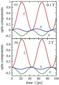
Figure 1: Free evolution of $\sigma_{R}^{i}(t)$ for all spin components, as marked near the plots for the initial spin-up case: (a) for weak field $H_{z}=0.1$ T (here we use $\alpha=1.0\cdot 10^{-9}$ eVcm, $\beta=0$), (b)-relatively strong field $H_{z}=2$ T. The probability to find the electron in the right dot $w_{R}(t)$ almost coincides with $\sigma_{R}^{z}(t)$, and only a slight spin deviation from the initial value due to SO coupling is observed.

Hamiltonian and time evolution. We describe a one-dimensional double QD by the Hamiltonian, similar to suggested in Ref.[17], for the particle with mass $m$ in a quartic potential

$$U(x)=U_{0}(-2(x/d)^{2}+(x/d)^{4}),$$ (1)

where the minima located at $d$ and $-d$ are separated by a barrier of height $U_{0}$. We assume that the barrier is opaque enough to ensure that the ground state is close to the even linear combination of the oscillator states located near the minima. The frequency of the single-dot harmonic oscillator is determined by $\omega_{0}=2\sqrt{2U_{0}}/d\sqrt{m}$ and the corresponding oscillator length $a_{0}=\sqrt{\hbar/m\omega_{0}}$. The interdot semiclassical tunneling probability in the ground state:

$$w_{t}=\exp\left[-\frac{8\sqrt{2}}{3}\frac{\sqrt{mU_{0}}d}{\hbar}\right]$$ (2)

is small. The tunneling splits the ground state with the energy close to $-U_{0}+\hbar\omega_{0}/2$ by $\Delta E_{g}$ of the order of $\hbar\omega_{0}w_{t}.$ The high-energy states with the orbital quantum number $n\gg 1$ can be treated semiclassically for the potential $U(x)=U_{0}(x/d)^{4},$ yielding the eigenenergy:

$$E_{n}=\left(\frac{3\Gamma^{2}(3/4)}{2\sqrt{2\pi}}\right)^{4/3}n^{4/3}\hbar\omega_{0}\left(\frac{\hbar\omega_{0}}{U_{0}}\right)^{1/3},$$ (3)

where $\Gamma$ is the gamma function. Correspondingly, the maximum semiclassical momentum achieved when the electron passes the vicinity of the $x=0$ point, is $p_{n}^{\max}\sim\sqrt{2mE_{n}}\sim n^{2/3}\left(\hbar\omega/U_{0}\right)^{1/6}\hbar/a_{0}.$

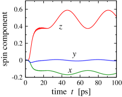
Figure 2: Evolution of the spin components (as marked near the plots) for initial spin-up state in a weak magnetic field $H=0.1$ T, where the spin is influenced only by the SO coupling. As in fig.1(a), here we use $\alpha=1.0\cdot 10^{-9}$ eVcm, $\beta=0$. The external field is weak, $f=1/8$, and the pulse duration $T=25$ ps.

For the system in a static magnetic field $H_{z}$ and driven by an external electric field $\mathcal{E}(t)$ directed along the $x$-axis, the Hamiltonian is the sum of three terms $H=H_{0}+H_{\mathrm{so}}+\widetilde{V}$ with:

$$H_{0} = \frac{p_{x}^{2}}{2m}+U(x)+\frac{g}{2}\mu_{B}\sigma_{z}H_{z}$$ (4)

$$H_{\mathrm{so}} = \left(\beta\sigma_{x}+\alpha\sigma_{y}\right)p_{x},\qquad\widetilde{V}=-e\mathcal{E}(t)x,$$ (5)

where $e$ is the electron charge, and $\sigma_{i}$ are the Pauli matrices. The effect of $H_{z}$ is described by the Zeeman term only, where $g$ is the Landé factor. The SO interaction is the sum of bulk-originated Dresselhaus $\left(\beta\right)$ and structure-related Rashba $\left(\alpha\right)$ terms. The corresponding velocity operator

$$v\equiv\dot{x}=\frac{{\rm i}}{\hbar}[H_{0}+H_{\mathrm{so}},x]={p_{x}}/{m}+\beta\sigma_{x}+\alpha\sigma_{y}.$$ (6)

is spin-dependent.

To describe the driven motion we use the following approach. First, we diagonalize exactly the Hamiltonian $H_{0}+H_{\rm so}$ in the truncated basis of spinors $\psi_{n}(x)\left|\sigma\right>$ with corresponding eigenvalues $E_{n\sigma}$ and obtain the new basis set $\left|\psi_{\mathbf{n}}\right>$ where bold $\mathbf{n}$ incorporates the corresponding spin index. The first four low-energy states are then defined as: $\left|\psi_{\mathbf{1}}\right>=\psi_{1}(x)\left|\uparrow\right>$, $\left|\psi_{\mathbf{2}}\right>=\psi_{1}(x)\left|\downarrow\right>$, $\left|\psi_{\mathbf{3}}\right>=\psi_{2}(x)\left|\uparrow\right>$, and $\left|\psi_{\mathbf{4}}\right>=\psi_{2}(x)\left|\downarrow\right>$.

Since the energy $E_{ns}$ increases as $n^{4/3}$, the truncated basis is sufficient for the purposes we consider below. Then, we build in this basis the matrix of the Hamiltonian $\widetilde{V}$ and study the full dynamics with the wavefunctions in the form:

$$\left|\Psi\right\rangle=\sum_{\mathbf{n}}\xi_{\mathbf{n}}(t)e^{-{\rm i}E_{\mathbf{n}}t/\hbar}\left|\psi_{\mathbf{n}}\right\rangle.$$ (7)

The time dependence of $\xi_{\mathbf{n}}(t)$ with $\widetilde{V}=-e\mathcal{E}(t)x$ is calculated as:

$$\frac{d}{dt}\xi_{\mathbf{n}}(t)={\rm i}\frac{e}{\hbar}\mathcal{E}(t)\sum\xi_{\mathbf{m}}(t)x_{\mathbf{nm}}e^{-{\rm i}\left(E_{\mathbf{m}}-E_{\mathbf{n}}\right)t/\hbar},$$ (8)

where $x_{\mathbf{nm}}\equiv\left\langle\psi_{\mathbf{n}}\right|\widehat{x}\left|\psi_{\mathbf{m}}\right\rangle$. Since we do not assume a periodic driving field, we do not resort to the Floquet method [12, 18], but use the direct numerical calculation instead. Taking into account that we are interested in a relatively short-term dynamics, we neglect momentum relaxation. This approximation is allowed at low temperatures and low excitation energies.

The spin-dependence of the matrix element of coordinate responsible for the spin dynamics can be seen from expression ${\rm i}({E_{\mathbf{n}}-E_{\mathbf{m}}})x_{\mathbf{nm}}$ $={\hbar}\left\langle\psi_{\mathbf{n}}\right|\widehat{v}\left|\psi_{\mathbf{m}}\right\rangle,$ and the spin-dependent terms in the velocity in (6).

Observables and results. Our main goal is to calculate the probability-

$$\rho(x,t)=\Psi^{\dagger}(x,t)\Psi(x,t)$$ (9)

and spin-

$$S_{i}(x,t)=\Psi^{\dagger}(x,t)\sigma_{i}\Psi(x,t),$$ (10)

density using (8). With these distributions we find the gross quantities for the right QD:

$$w_{R}(t) = \int_{0}^{\infty}\rho(x,t)dx,$$ (11)

$$\sigma_{R}^{i}(t) = \int_{0}^{\infty}S_{i}(x,t)dx,$$ (12)

where $w_{R}(t)$ is the probability to find electron and $\sigma_{R}^{i}(t)$ is the expectation value of spin component. As the electron wavefunction at $t=0$ we take linear combinations of four low-energy states. The initial state is localized in the left QD, and we choose combinations: $\xi_{\mathbf{1}}=\xi_{\mathbf{3}}=1/\sqrt{2}$ for the spin-up, and $\xi_{\mathbf{2}}=\xi_{\mathbf{4}}=1/\sqrt{2}$ for the spin-down states.

We consider a structure with $d=25\sqrt{2}$ nm and $U_{0}=10$ meV, with the corresponding oscillator length $a_{0}=23$ nm. The four lowest spin-degenerate energy levels are $E_{1}=3.938$ meV, $E_{2}=4.030$ meV, $E_{3}=9.782$ meV, $E_{4}$=11.590 meV counted from the bottom of a single QD. The tunneling splitting $\Delta E_{g}=E_{2}-E_{1}=0.092$ meV. The parameters of the SO coupling are assumed to be $\alpha=1.0\cdot 10^{-9}$ eVcm, $\beta=0.3\cdot 10^{-9}$ eVcm. We assume the magnetic field $H_{z}=2$ T, which produces the Zeeman spin splitting of the levels $\Delta_{z}=E_{n\downarrow}-E_{n\uparrow}=0.054$ meV for the Landé-factor of electron in GaAs $g=-0.45$.

In numerical calculations the basis of 20 states with the energies up to 42 meV was employed. We consider the period of time evolution $0\leq t\leq 100$ ps tracking the system in the transient and following stationary processes.

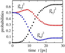
Figure 3: Evolution of the components of the wave function (as marked near the plots) for initial spin-down state. The external field is characterized by $f=1/2$, and the pulse duration $T=25$ ps.

We begin with the analysis of the free evolution, where $\widetilde{V}=0$. The results are presented in fig.1 for two magnetic fields. One can see the free tunneling Rabi oscillations with the period $T_{R}$ of approximately 50 ps and the corresponding spin oscillations. Figure 1 shows that no spin flip can be achieved in the tunneling at this system parameters. Moreover, $w_{R}(t)$ (not shown in the figure) and $\sigma_{R}^{z}(t)$ almost coincide, confirming that tunneling by itself does not lead to a considerable spin dynamics. The similarity of the free motion pictures for $H_{z}=0.1$ and $H_{z}=2$ T shows that the $z-$axis field, even producing the Zeeman splitting comparable with the tunneling splitting of the ground state, does not modify the tunneling. In the tunneling, spin precession mainly around the $y$-axis due to the Rashba SO term is observed. The precession angle defined for this case as $\phi={\rm atan}\left(\sigma_{R}^{y}/\sigma_{R}^{z}\right)$ achieves the maximum $\phi_{\max}\approx 0.25$ at $t=T_{R}/2$. This number should be compared with the precession angle for the classical motion, where displacement of electron by the distance $l$ leads to the precession angle $\phi_{\rm cl}(l)=2ml\alpha/\hbar^{2}$. For given geometry of the structure with $l=2d$, one obtains $\phi_{\rm cl}(2d)=1.2$, considerably larger than $\phi_{\max}$. This implies that combination of tunneling and SO coupling cannot be treated semiclassically being strongly different from what can be expected. Namely, due to the enhanced role of the tunneling the precession angle becomes considerably smaller. Here a general remark is appropriate. It was suggested [19] and analyzed [20, 21] how to use the Larmor spin precession in magnetic field as the measure of the time electron spends inside a barrier. In the presence of SO coupling every electron has an associated momentum-dependent magnetic field acting on the spin. Whether the spin precession in this field can be used as a measure of tunneling time is an interesting question.

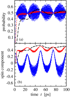
Figure 4: Evolution of the probabilities $w_{R}(t)$ (a) and $\sigma_{R}^{i}(t)$ (b) under the electric field pulse with $f=1/8$, $f=1/2$, and $f=2$ for the initial spin-up state. The pulse durations $T=25$ ps. Dashed line shows the $f=1/8$ regime. With the increase in the pulse field, the motion becomes less regular, and more high-energy component contribute into the dynamics.

As the external perturbation we consider half-period electric field pulses in the form $\mathcal{E}(t)=\mathcal{E}_{0}\sin(\pi t/T)$ for $0<t<T$. For the pulse duration we assume $T=T_{R}/2.$ The spectral width of the pulse covers both the spin and the tunneling splitting of the ground states, thus, driving the spin and orbital dynamics simultaneously. Chosen pulse duration satisfies the condition $T\omega_{0}\gg 1$, that is the corresponding frequencies are much less than the energy difference between the orbital levels corresponding to a single dot, and, therefore, the high energy states follow the perturbation adiabatically. The field strength is characterized by parameter $f$ such that $e\mathcal{E}_{0}\equiv f\times U_{0}/2d$. For the coupling we consider three regimes: (i) a relatively weak field ($f\ll 1$) where the shape of the quartic potential remains almost intact, and the tunneling is still crucially important, (ii) intermediate filed, and (iii) strong field $f>1$, where the perturbation already considerably changes the low-energy part the spectum.

As the first example, we consider the pulse-driven evolution in a weak magnetic field $H_{z}=0.1$ T, where the spin dynamics is determined mainly by the SO coupling. The dynamics is shown in fig.2. Even a weak field strongly changes the observables: in the rich transient dynamics it quickly almost equilazes the probabilities to find electron in the right and left dot, and the subsequent oscillations of probability around 0.5 value occur. Same behavior is demonstrated by the spin components - they weakly oscillate around mean value since the electron travels a shorter distance during the density oscillations, however, a similar to fig.1 spin polarization $\sigma_{R}^{i}(t)/w_{R}(t)$ is achieved.

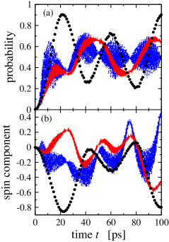
Figure 5: Evolution of the probabilities $w_{R}(t)$ (a) and $\sigma_{R}^{i}(t)$ (b) under the electric field pulse with $f=1/8$, $f=1/2$, and $f=2$ for the initial spin-down state. Circle symbol line corresponds to the $f=1/8$ regime. The pulse durations $T=25$ ps. Similarly to fig.4, with the increase in the pulse field, the motion becomes less regular, and more high-energy component contribute into the dynamics. However, the dynamics is much richer here. For the $f=1/2$ case the main underlying $|\xi_{\mathbf{n}}|^{2}$ are shown in fig.3.

We present driven dynamics in the Hilbert space with the coefficients $\xi_{\mathbf{n}}$ for $f=1/2$ in fig.3. This picture shows only the largest remaining after the end of the pulse components, demonstrating the orbital and spin dynamics, equilibrating the probably density as $|\xi_{\mathbf{4}}|^{2}$ decreases with respect to $|\xi_{\mathbf{2}}|^{2}$, and causing the spin evolution by increasing $|\xi_{\mathbf{1}}|^{2}$.

The observables for the pulses with different ${\mathcal{E}}_{0}$ are shown in fig.4 and fig.5 for the initial spin-up and spin-down states. Comparison of fig.4 and fig.5 shows that the time-dependence of the spin density, and, more important, of the probability is quite different for different initial spin states despite the fact that in both cases the dynamics consists of low- frequency motion corresponding to the spectrum of the four low-energy states superimposed by the set of very-high frequency oscillations due to the involvement of the higher-energy states. For the spin-up initial state, the weak and moderate external field just equalizes the probability for the electron to occupy the left and the right dots, and then only high-frequency oscillations occur. For the initial spin-down state, the dynamics is much richer: the low-frequency oscillations with a large amplitude are clearly seen at long times. In both cases the amplitude of the fast oscillations increases with the increase in the field. The difference between these two regimes is non-trivial and can be understood as follows. The coupled spin-charge dynamics is considerably determined by the difference in the energy of the nearest spin up and spin down states with opposite parity. The larger is the distance, the less efficient is the SO coupling for the coupled dynamics both in the low- and high-frequency domains. For the low-energy spin-up states it is $\left|E_{\mathbf{4}}-E_{\mathbf{1}}\right|=\Delta E_{g}+\Delta_{z}$, while for the initial spin-down state it is $\left|E_{\mathbf{3}}-E_{\mathbf{2}}\right|=\Delta E_{g}-\Delta_{z}$. For $H_{z}=2$ T, $\left(\Delta E_{g}-\Delta_{z}\right)/\left(\Delta E_{g}+\Delta_{z}\right)\approx 0.25$, making the spin flip at the given spectrum of the pulse, for the latter case easier, and the spin dynamics richer.

To have a better insight into the evolution of the spin density, we illustrate the dynamics by a plot of $S_{z}(x,t)$ in fig.6 for pulse durations $T=12$ and $T=25$ ps, $f=2$ and the initial spin-down state. The figure shows that for the shorter $T=12$ ps pulse, the $S_{z}$ component in the right dot $(x=d)$ is positive at most of the time after the end of the pulse, illustrating the controlled spin flip accompanying the electron transfer. By moving along the time axis at $x=d$ we follow oscillations of the $S_{z}$ component consistent with the free tunneling on the scale of $T_{R}$. As for the evolution under the longer pulse $T=25$ ps shown in the lower panel of fig.6, the shape of $S_{z}(x,t)$ remains qualitatively the same, however the details of the distribution in the right dot are different. Namely, the dominating parts of the profile correspond to the negative $S_{z}$ at all times at $x\approx d$. This remarkable difference between the results for two pulse durations provides a good illustration for the interplay of a driven spin-and-charge motion and the tunneling occurring simultaneously. Namely, the stronger and the longer the electric pulse is, the more overall changes it provides for the coupled charge and spin dynamics. Since the spin evolution is the rotation, a too short (or a too weak) electric pulse may ”under-rotate” the spin with respect to the desirable state, as we have seen earlier for the weak pulses. A too strong (or a too long) electric pulse can ”over-rotate” the spin, which may pass the desired flipped state in the neighboring dot. This observation illustrated in fig.6 suggests to carefully control and adjust both the strength and duration of the electric pulses required for the controlled spin manipulation in heterostructures with significant SO coupling.

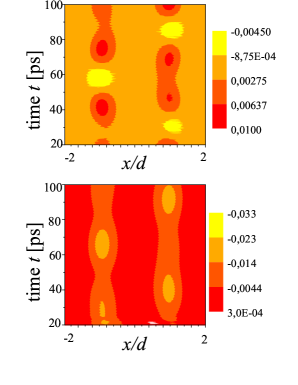
Figure 6: Evolution of the spin densities under the strong electric field $f=2$ pulse for two pulse durations $T=12$ ps (upper panel) and $T=25$ ps (lower panel). The variation in the pulse duration leads to the different outcome for the dominating final $S_{z}$ of the transferred electron.

Conclusions. We have studied the full driven quantum spin and charge dynamics of a spin qubit in one-dimensional double single-electron QD with SO coupling. Equations of motion in a pulsed electric field have been solved numerically exactly in a finite basis set in the regimes of relatively weak, moderate, and relatively strong coupling. The dynamics is strongly determined by the pulse amplitude and duration. The results show that the time dependence of the spin and charge distributions are strongly irregular with the spin-dependent evolution in the charge density pattern. Electron spin flip can be achieved at certain pulse durations and amplitudes. These conclusions emphasize the importance of the SO coupling which should be taken into account in experimental and technological realizations of spin-based qubits.

D.V.K. is supported by the RNP Program of Ministry of Education and Science RF (Grants No. 2.1.1.2686, 2.1.1.3778, 2.2.2.2/4297, 2.1.1/2833), by the RFBR (Grant No. 09-02-1241-a), by the USCRDF (Grant No. BP4M01), by ”Researchers and Teachers of Russia” FZP Program NK-589P, and by the President of RF Grant No. MK-1652.2009.2. EYS is supported by the University of Basque Country UPV/EHU grant GIU07/40 and MCI of Spain grant FIS2009-12773-C02-01. The authors are grateful to L.V. Gulyaev for technical assistance.

References

- [1] Kohler S., Lehmann J., and Hänggi P., Physics Reports 406, (2005) 379.
- [2] Burkard G., Loss D., and DiVincenzo D. P., Phys. Rev. B 59, (1999), 2070.
- [3] Rashba E. I. and Efros Al. L., Phys. Rev. Lett. 91, (2003) 126405.
- [4] E. I. Rashba and Al. L. Efros, Appl. Phys. Lett. 83, (2003) 5295.
- [5] Nowack K.C., Koppens F.H.L., Nazarov Yu.V., and Vandersypen L.M.K., Science 318, (2007) 1430.
- [6] Pioro-Ladriere M., Obata T., Tokura Y., Shin Y.-S., Kubo T., Yoshida K., Taniyama T., and Tarucha S., Nature Physics 4, (2008) 776.
- [7] Semenov Y. G. and Kim K. W., Phys. Rev. Lett. 92, (2004) 026601; Semenov Y. G. and Kim K. W., Phys. Rev. B 75, (2007) 195342.
- [8] Stano P. and Fabian J., Phys. Rev. Lett. 96, (2006) 186602; Stano P. and Fabian J., Phys. Rev. B 72, (2005) 155410; Stano P. and Fabian J., Phys. Rev. B 74, (2006) 045320.
- [9] Sánchez D. and Serra L., Phys. Rev. B 74, (2006) 153313; Crisan M., Sánchez D., López R., Serra L., and Grosu I., Phys. Rev. B 79, (2009) 125319.
- [10] Lü C., Zülicke U., and Wu M. W., Phys. Rev. B 78, (2008) 165321.
- [11] Romano C.L., Tamborenea P.I., and Ulloa S.E., Phys. Rev. B 74, (2006) 155433.
- [12] Jiang J. H. and Wu M. W., Phys. Rev. B 75, (2007) 035307; Jiang J. H., Wu M. W., and Zhou Y., Phys. Rev. B 78, (2008) 125309.
- [13] Khomitsky D. V. and Sherman E. Ya., Phys. Rev. B 79, (2009) 245321.
- [14] Lin W.A. and Ballentine L.E., Phys. Rev. Lett. 65, (1990) 2927; Lin W.A. and Ballentine L.E., Phys. Rev. A 45, (1992) 3637.
- [15] Tameshtit A. and Sipe J. E., Phys. Rev. E 51, (1995) 1582; Tameshtit A. and Sipe J. E., Phys. Rev. A 47, (1993) 1697.
- [16] Murgida G. E., Wisniacki D. A., and Tamborenea P. I., Journal of Modern Optics 56, (2009) 799; Villas-Boas J. M., Ulloa S. E., and Studart N., Phys. Rev. B 70, (2004) 041302(R).
- [17] Romano C. L., Ulloa S. E., and Tamborenea P. I., Phys. Rev. B 71, (2005) 035336.
- [18] Shirley J. H., Phys. Rev. 138, (1965) B979.
- [19] Baz A.I., Sov. Journ. Nucl. Phys. 5, (1967) 161.
- [20] Büttiker M., Phys. Rev. B 27, (1983) 27.
- [21] Sokolovski D. and Baskin L.M., Phys. Rev. A 36, (1987) 4604; Sokolovski D. and Connor J.N.L., Phys. Rev. A 47, (1993) 4677.