Bulk File Download Throughput in a Single Station WLAN with Nonzero Propagation Delay

Abstract

We analyze TCP-controlled bulk file transfers in a single station (STA) WLAN with nonzero propagation delay between the file server and the WLAN. Our approach is to model the flow of packets as a closed queueing network (BCMP network) with 3 service centres, one each for the Access Point (AP) and the STA, and the third for the propagation delay. The service rates of the first two are obtained by analyzing the WLAN MAC. Simulations show a very close match with the theory.

I Introduction

We consider an infrastructure wireless network employing the IEEE 802.11 DCF mechanism and carrying TCP-controlled file downloads. In this paper, we study analytical models for evaluating the performance of TCP-controlled downloads with non zero round trip propagation delays. In the literature, many works address the analysis of TCP flows in wireless networks. However very few consider non negligible round trip propagation delays in their models.

Our approach can be summarized as follows. First, we consider only two nodes in the network -an AP and an STA. We obtain expressions for AP and STA throughput in the absence of propagation delays. We consider that all the wireless medium specific proprieties of the system are encapsulated in these expressions. Next, we include the effect of RTPD by using a closed queueing network. We validate our model by comparison with various simulated quantities, such as mean number of packets in the AP, STA and in flight. Our numerical results of model matches with maximum error of 1.87 % error.

Outline of the paper: Section II outlines related work. In Section III we We summarize out modelling assumption with the system model. In Section IV we provide analysis for throughputs in case of two contending nodes. In Section V, we validate model by comparing with the results obtained from the Qualnet network simulator. In Section VI we discuss the results and conclude the paper.

II Related Work

Numerous models and analyses have been proposed for wireless networks with TCP-controlled traffic, but very few consider propagation delays. In [5], RTT is considered for modelling the TCP traffic in WLAN, but the authors’ interest was in providing analysis supporting the service differentiation feature in 802.11e. The authors ensured fairness among TCP data packets and TCP ACKs by utilizing the different Access Categories in 802.11e, and their analysis exploited this fairness to show that service differentiation is possible.

A detailed analysis and modelling of the aggregate throughput of TCP flows in WLANs for a single rate access point is given in [1] and [8] by assuming negligible or zero round trip time (RTT). Similarly, the performance of the AP is evaluated in the multi rate case in [2], [3] and [4]. However these works also ignore the RTT.

An extension of this model in [2] considers two rates of association with long file uploads from STAs to a local server. The multirate case is considered in [3], and arbitrary TCP windows are allowed in [4]. [9] and [10] present another analysis of a scenario of TCP-controlled upload and download file transfers, with UDP traffic. They ignored the RTT effect on the behaviour of the network. The letter [11] gives the average value analysis of TCP performance with upload and download traffic with out considering RTT. In [12], a finite buffer AP with TCP traffic in both upload and download directions is analysed with delayed and undelayed ACK cases. They consider server system located on the Ethernet to which the AP is connected and hence number of packets “in flight” outside the WLAN is ignored.

[13] and [14] provide models in finite load conditions by approximating the packet arrival precess at the STAs as a Poisson process. [13] extended saturated model proposed in [15] to non saturated model by introducing a term for probability of queue being empty. [14] models every STA with M/G/1 queue considers the propagation delay as the delay in transmission of packet in wireless medium, and not the time spent in reaching the WLAN from the server.

[16] provides an analysis for a given number of STAs and maximum TCP receive window size by using the well known $p$ persistent model proposed in [7]. However, both [16] and [7] consider no RTT effect in the traffic.

[17] considers HTTP traffic. A queuing model is proposed to compute the mean session delay in the presence of short-lived TCP flows and the impact of TCP maximum congestion window size on this delay is studied. The analysis is extended to consider delayed ACKs asw well.

III System Model

We consider a WLAN in which an STA is associated with an AP as shown in Figure 1. We consider long-lived TCP connections having bulk data to send. That is, we focus on large file transfers. The server is far away from the LAN. Hence, there is propagation delay between the AP and the server. Every packet experiences this delay. Figure 1 shows the direction of TCP flow. The STA has a single TCP connection to download long files from the server. Further, because of bulk transfer scenario, we can assume that the TCP flow is in the steady state. We assume that the application at the receiver reads data from the socket receive buffer at the rate at which it is received from the network. Hence, the TCP ACK packets always advertise the maximal TCP receive window size. Therefore, TCP startup transients can be ignored. Also, TCP timeouts do not occur.

The AP and the STA contend for the channel using the DCF mechanism. We assume that there are no link errors. Packets in the medium are lost only due to collisions between transmission attempts of AP and STA. Further, we assume that all the nodes use the RTS-CTS mechanism while sending packets, and use basic access to send ACK packets. As soon as the station receives a data packet, it generates an ACK packet without any delay and it is enqueued at the MAC layer for transmission. We assume that all the nodes have sufficiently large buffers, so that packets are not lost due to buffer overflow.

Figure 1: The network and traffic configurations. An STA is downloading a long file from a server through an AP.

IV Analysis

Because two entities, i.e., the AP and the STA, are contending for the channel, we can consider probability of attempt as $\beta_{2}$, as in [6]. This amounts to assuming that both AP ans STA are backlogged permanently, i.e., that saturation conditions apply. Current TCP implementations use very large windows (window scaling option), and with these, our assumption is justifiable.

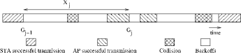
Figure 3: An example of activities in a channel.Here, $G_{j}$ are random time instants at which successful transmissions complete for a packet. Random duration $X_{k}$ denotes the $j^{th}$ contention cycle $[G_{j-1},G_{j})$. Each contention cycle consists of one or more back off periods and collisions but ends with a successful transmission.

Figure 3 shows one possible sample path of events on the wireless channel in the WLAN with an AP and an STA. The random epochs $G_{j}$ indicate the end of the $j^{th}$ successful transmission from either the AP or the STA.

Let $T_{s}AP$ be the time taken by the AP to transmit one packet TCP packet including MAC and PHY headers. This can be obtained by using parameter shown in Table I. We have

$$\begin{split}TsAP&=T_{p}+T_{PHY}+\frac{L_{RTS}}{r_{c}}+T_{SIFS}\\ &+T_{p}+T_{PHY}+\frac{L_{CTS}}{r_{c}}+T_{SIFS}+T_{p}+T_{PHY}\\ &+\frac{L_{MAC}+L_{IPH}+L_{TCPH}+L_{TCP}}{r_{d}}+T_{SIFS}\\ &+T_{p}+T_{PHY}+\frac{L_{ACK}}{r_{c}}+T_{DIFS}\end{split}$$ (1)

As data transmission follows an RTS-CTS exchange, the lengths of the RTS and CTS packets, as well as $T_{SIFS}$, are used in (1)

Parameter	Symbol	Value
PHY data rate	$r_{d}$	11 Mbps
Control rate	$r_{c}$	2 Mbps
PLCP preamble time	$T_{p}$	$144\mu s$
PHY Header time	$T_{PHY}$	$48\mu s$
MAC Header size	$L_{MAC}$	34 bytes
RTS Header size	$L_{RTS}$	20 bytes
CTS Header size	$L_{CTS}$	14 bytes
MAC ACK Header size	$L_{ACK}$	14 bytes
IP Header size	$L_{IPH}$	20 bytes
TCP Header size	$L_{TCPH}$	20 bytes
TCP ACK Packet size	$L_{TCP-ACK}$	20 bytes
TCP data payload size	$L_{TCP}$	1460 bytes
System slot time	$\delta$	$20\mu s$
DIFS time	$T_{DIFS}$	$50\mu s$
SIFS time	$T_{SIFS}$	$10\mu s$
EIFS time	$T_{EIFS}$	$364\mu s$
Min. Contention Window	$CW_{min}$	31
Max. Contention Window	$CW_{max}$	1023

TABLE I: Values of Parameters used in Analysis and Simulation

We note that whenever there is a collision between RTS packet from the AP and a TCP-ACK packet from the STA, the channel time wasted is that due to the TCP-ACK packet. This is because the RTS packet is smaller than a TCP-ACK packet as given in I. Let $T_{c}$ be the time spent in collision.

$$\begin{split}T_{c}=T_{p}+T_{PHY}+\frac{L_{MAC}+L_{IPH}+L_{TCP-ACK}+L_{TCP}}{r_{d}}\\ +T_{EIFS}\end{split}$$ (2)

In the above expressions, we have considered that TCP data packets are larger than the RTS threshold and hence the AP uses the RTS-CTS access mechanism. Since TCP-ACKs are smaller, the STA uses the basic access mechanism. Let $T_{sSTA}$ be the time taken by the STA to transmit one TCP ACK packet, including MAC and PHY overhead. We have

$$\begin{split}T_{sSTA}&=T_{p}+T_{PHY}\\ &+\frac{L_{MAC}+L_{IPH}+L_{TCPH}+L_{TCP-ACK}}{r_{d}}\\ &+T_{SIFS}+T_{P}+T_{PHY}+\frac{L_{ACK}}{r_{c}}+T_{DIFS}\end{split}$$ (3)

The probability that the AP wins the contention in the first attempt is $\beta_{2}(1-\beta_{2})$; let this be denoted as $\alpha_{2}$.

Let the mean back-off length at $i^{th}$ attempt be

$$EB^{i}=\frac{2^{i}CW_{min}+1}{2}$$

Let $s_{sAP}^{k}$ be the mean time taken by AP to transmit a TCP data packet after $k$ collisions. This can be obtained as

$$s_{AP}^{k}=\sum_{i=1}^{k+1}EB^{i}+kT_{c}+T_{sAP}$$ (4)

which is mean weighted sum of conditional means. In the above Equation, if the back-off window reaches $CW_{max}$, it stays fixed at $CW_{max}$.

Also the probability of $k$ times collisions and the success at $(k+1)^{th}$ is $(1-\alpha_{2})^{k}\alpha_{2}$.

Hence the mean service time at the AP, with the STA is also contending for the channel is given by

$$s_{AP}=\sum_{i=1}^{\infty}s_{AP}^{k}(1-\alpha_{2})^{k}\alpha_{2}$$ (5)

Similarly, the time taken by the STA to transmit a TCP-ACK packet after $k$ collision is

$$s_{STA}^{k}=\sum_{i=1}^{k+1}EB^{i}+kT_{c}+T_{sSTA}$$ (6)

and the mean service time at the STA is

$$s_{STA}=\sum_{i=1}^{\infty}s_{STA}^{k}(1-\alpha_{2})^{k}\alpha_{2}$$ (7)

IV-A BCMP network

Having obtained the service rate of the AP and STA, we can model the scenario shown in Figure 1 as a BCMP closed queueing network with three service centers [18]. The queues in this network representing the AP and STA are First Come First Served queues (FCFS), which are ‘Type 1’ service centres in the terminology of [18]. Similarly, the queue representing round trip propagation delay (RTPD) is an infinite server queue with deterministic service time, which is a ‘Type 3’ service center.

Let us consider $W$ packets in this network. Let $w_{1}$ packets to be at center 1; that is, $w_{1}$ among $W$ packets are at the AP. Also, let $w_{2}$ out of $W$ packets be at center 2, which is an STA. Similarly, the remaining packets, say $w_{3}$, are in the delay center. The state of the network can be represented by $S=(x_{1},x_{2},x_{3})$, as in [18]. The definitions of $x_{1},x_{2}$ and $x_{3}$ depend on the type of the service center and are given in [18].

Every transition is both a departure from one center and an arrival at another center. For every $i$, let $e_{i}$ be the fraction of transitions that are arrivals at (departures from) center $i$. Let $v_{i^{\prime},i}$ be the probability that a customer at center $i^{\prime}$ goes to center $i$. We have $v_{1,2}=v_{1,2}=v_{1,2}=1$. From [19], $e_{i}$ unique solution (that sums to 1) of the following system of equation

$$e_{i}=\sum_{i}(e_{i^{\prime}})v_{i^{\prime},i}$$ (8)

Hence, $e_{i}=\frac{1}{3}$. Every packet moves from one service center to another.

Figure 2: An equivalent BCMP closed queueing network model for the scenario given in Figure 1 considering packets as customers. Total number of customers is equal to the maximum receive window advertised by TCP receiver

By the BCMP theorem [18], the equilibrium probabilities are given by

$$P(S=x_{1},x_{2},x_{3})=Cd(S)f_{1}(x_{1})f_{2}(x_{2})f_{2}(x_{3})$$ (9)

where $C$ is the normalizing constant chosen to make the equilibrium state probabilities sum to 1. $d(S)$ is a function of the number of customers in the system, and $f_{i}$ is a function that depends on the type of service center $i$.

From [18], for the FCFS server, i.e., AP, center 1,

$$f_{1}(x_{1})=\left(s_{AP}\right)^{n_{1}}e_{1}$$ (10)

for the FCFS server STA, center 2,

$$f_{2}(x_{2})=\left(s_{STA}\right)^{n_{2}}e_{2}$$ (11)

and for the infinite server, delay model, center 3, is represented by cascading of $c$ number of exponential servers in $c$ stages with service rate $\frac{1}{c\times t_{RTPD}}$ method in [20] (by considering large value of $c$) gives

$$f_{3}(x_{3})=\Pi_{l=1}^{c}\left(\frac{e_{3}}{c\times\tau_{RTPD}}\right)^{n_{3,l}}(1/n_{3,l}!)$$ (12)

For a closed network, $d(S)=1$.

The average number of packets at the AP, $n_{AP}$, the average number of packets at the STA, $n_{STA}$, and the average number of packets in propagation, $n_{RTPD}$ can be obtained by finding the marginal distributions from (9).

From Figure 2 the total number of packets is distributed among the three service centers.

$$n_{AP}+n_{STA}+n_{RTPD}=W$$

Let the throughput in the closed network of Figure 2 be $t_{H}$. Then, applying Little’s Theorem to service center 3, we have

$$n_{RTPD}=t_{H}\times t_{RTPD}$$ (13)

V Evaluation

In this section, we compare the numerical results obtained from our analysis with those obtained from simulation using the the Qualnet 4.5 network simulator [21]. The parameters used were taken from the IEEE 802.11b standard and are given in Table I. The error bars in the simulation curves denote 95% confidence intervals. We have taken the STA to be associated at rate 11 Mbps, with control packet transmission rate at 2 Mbps. RTPD is varied from 10ms to 90ms in step of 10ms. TCP Receive window is taken as 70 packets.

In Table II, the average number of packets in the AP obtained from analysis and simulations are shown.

	Analysis	Simulation
RTPD(ms)	Packets	Mean	Max	Min
10	34.75	34.77	37.40	32.14
20	29.89	29.93	33.05	26.81
30	31.52	31.58	33.47	29.66
40	28.85	28.90	30.68	27.12
50	26.92	26.97	28.79	25.14
60	26.78	26.84	28.22	25.46
70	23.84	23.89	25.19	22.59
80	22.34	22.40	23.46	21.33
90	20.51	20.56	21.45	19.67
100	19.27	19.32	19.94	18.71

TABLE II: Number of packets in AP buffer at rate 11Mbps for different values of RTPD.

	Analysis	Simulation
RTPD(ms)	Packets	Mean	Max	Min
10	3.19	3.19	3.21	3.18
20	6.37	6.361	6.39	6.33
30	9.55	9.536	9.59	9.48
40	12.74	12.723	12.78	12.66
50	15.92	15.89	15.96	15.82
60	19.06	19.02	19.12	18.92
70	22.22	22.168	22.31	22.03
80	25.44	25.381	25.52	25.25
90	28.57	28.492	28.61	28.37
100	31.65	31.557	31.71	31.4

TABLE III: Number of packets in “in flight” for different values of RTPD.

	Analysis	Simulation
RTPD(ms)	Packets	Mean	Max	Min
10	32.07	33.40	36.8	30.00
20	33.74	33.14	35.46	30.82
30	28.93	27.95	29.88	26.03
40	28.40	28.55	30.17	26.94
50	27.16	27.99	29.99	25.98
60	24.16	24.12	25.44	22.79
70	23.94	23.36	24.69	22.03
80	22.22	22.59	23.69	21.47
90	20.93	20.21	21.42	18.99
100	19.09	19.41	20.04	18.78

TABLE IV: Number of packets in STAs buffer at rate 11 Mbps for different values of RTPD.

	Analysis		Simulation
RTPD(ms)	packets/s	Mean	Max	Min
10	320.26	320.34	321.47	319.21
20	319.54	319.75	320.97	318.54
30	319.45	319.64	321	318.29
40	319.38	319.57	321.2	317.95
50	319.07	319.15	320.46	317.86
60	318.85	319.11	320.55	317.68
70	318.49	318.75	320.34	317.17
80	318.41	318.56	319.81	317.33
90	318.32	318.45	319.71	317.21
100	318.3	318.53	320.01	317.06

TABLE V: Throughput of the AP with a single STA at rate 11 Mbps for different values of RTPD. TCP window = 100 packets

Figure 4: TCP throughput vs RTPD for TCP window 40 and 70 packets

Figure 5: TCP throughput vs TCP window for RTPD of 10 ms

Figure 6: Number of Packets in AP buffer. TCP window = 100 packets.

Figure 7: Number of Packets In Flight. TCP window = 100 packets.

In Tables V and Figures 4, 5, 6 and 7 comparisons between analytical and simulation values are given for 11Mbps to illustrate the accuracy of the analytical model.

VI Conclusion

In this paper we developed a simple analytical framework to obtain accurate closed-form expressions for the performance of the AP and STAs with persistent TCP connections in the presence of round trip propagation delay. We verified the accuracy of the analytical model with the simulation results.We consider that TCP in its steady state, the TCP advertised window is smaller than the TCP congestion window.

References

- [1] G. Kuriakose, S. Harsha, A. Kumar, and V. Sharma, “Analytical models for capacity estimation of IEEE 802.11 WLANs using DCF for Internet applications,” Wireless Networks, 2006.
- [2] Krusheel M and J. Kuri, “Performance Analysis of TCP Uploads in WLANs with Multiple Rates,” In Proceeding of National Conference on Communications 2009.
- [3] Pradeepa BK and J. Kuri, “ Aggregate Download Throughput for TCP-controlled long file transfers in a WLAN with multiple STA-AP association rates” http://arxiv.org/abs/1007.3229
- [4] Pradeepa BK and J. Kuri, “Aggregate AP Throughputs for Long File Transfers in a WLAN controlled by Inhomogeneous TCP Connections,” http://arxiv.org/abs/1009.0919
- [5] D. Leith, and P. Clifford, “Modelling TCP dynamics in wireless networks,” in Proceedings of Wirelesscom, 2005, pp. 906-911 vol.902.
- [6] A. Kumar, E. Altman, D. Miorandi, and M. Goyal, “New insights from a fixed point analysis of single cell IEEE 802.11 WLANs,” IEEE/ACM Transaction On Networking, Vol. 15, No 3, pp. 588-601, June 2007.
- [7] F. Cali, M. Conti, and E. Gregori, “Dynamic Tuning of the IEEE 802.11 protocol to achieve a Theoretical Throughput Limit,” IEEE/ACM Transaction On Networking, vol. 8 no. 6 pp. 785-799, Dec 2000
- [8] R. Bruno, M. Conti, and E. Gregori, “Throughput Analysis of TCP clients in Wi-Fi Hot Spot Networks,” Networking 2004, LNCS 2042, pages 626-637, 2004
- [9] R. Bruno, M. Conti, and E. Gregori, “Throughput Analysis and Measurements in IEEE 802.11 WLANs with TCP and UDP Traffic flows,” IEEE Transaction on Mobile Computing, vol.7, no.2, pp. 171-186, Feb. 2008.
- [10] R. Bruno , M. Conti, and E. Gregori, “An Accurate Closed-form formula for the throughput of long-lived TCP connections in IEEE 802.11 WLANs,” Computer Networks, vol. 52, pages. 199-212, 2008
- [11] R Bruno, M Conti, and E Gregori, “Average Value Analysis of 802.11 WLANs with Persistent TCP flows,” IEEE Communication Letters, vol.13, no.4, Apr. 2009.
- [12] O. Bhardwaj, G. V. V. Sharma, M. Panda, and A. Kumar, “Modeling finite buffer effects on tcp traffic over an ieee 802.11 infrastructure wlan,” Computer Networks, vol. 53, pages. 2855–2869, Nov 2009
- [13] K. Duffy, D. Malone, and D. J. Leith, “Modelling 802.11 Wireless Links,” In CDC-ECC ’05, volume 3, pages 6952-6957, 12-15 Dec 2005.
- [14] J.V. Sudarev, L.B. White, and S. Perreau, “Performance Analysis of 802.11 CSMA/CA for Infrastructure Networks under Finite Load Conditions,” In Local and Metropolitan Area Networks, 2005. volume 3, pages 1-6, 18-21 Sept 2005
- [15] G. Bianchi, “Performance analysis of the IEEE 802.11 distributed co- ordination function,” IEEE Journal on Selected Areas in Communications, Volume 18, Issue 3, March 2000, pp. 535-547
- [16] J. Yu, S. Choi, “Modeling and Analysis of TCP dynamics over IEEE 802.11 WLAN,” Proc. of the IFIP WONS,, pp. 154-161 Obergurgl, Austria, 2007.
- [17] D. Miorandi, A. Kherani, E. Altman, “A queueing model for HTTP traffic over IEEE 802. 11 WLANs,” Computer Networks, vol. 50, no. 1, pp. 63-79, 2006.
- [18] Baskett. F, Chandy. K. Mani, Muntz. R.R., Palacios, F.G. (1975). “Open, closed and mixed networks of queues with different classes of customers.” Journal of the ACM 22: 248–260. 1975.
- [19] Ronald W. Wolff, “Stochastic Modeling and the Theory of Queues,” Prentice Hall 1989.
- [20] Arnold O. Allen, “Probability, Statistics, and Queueing Theory with Computer Science Applications. Computer Science and Scientific Computing,” Academic Press, Inc., 2nd edition, 1990.
- [21] Qualnet Simulator, www.scalable-networks.com.