Doubly Exponential Solutions for Randomized Load Balancing Models with Markovian Arrival Processes and Phase-Type Service Times

Abstract

In this paper, we provide a novel matrix-analytic approach for studying doubly exponential solutions of randomized load balancing models (also known as supermarket models) with Markovian arrival processes (MAPs) and phase-type (PH) service times. We describe the supermarket model as a system of differential vector equations by means of density dependent jump Markov processes, and obtain a closed-form solution with a doubly exponential structure to the fixed point of the system of differential vector equations. Based on this, we show that the fixed point can be decomposed into the product of two factors inflecting arrival information and service information, and further find that the doubly exponential solution to the fixed point is not always unique for more general supermarket models. Furthermore, we analyze the exponential convergence of the current location of the supermarket model to its fixed point, and apply the Kurtz Theorem to study density dependent jump Markov process given in the supermarket model with MAPs and PH service times, which leads to the Lipschitz condition under which the fraction measure of the supermarket model weakly converges the system of differential vector equations. This paper gains a new understanding of how workload probing can help in load balancing jobs with non-Poisson arrivals and non-exponential service times.

Keywords: Randomized load balancing, supermarket model, matrix-analytic approach, doubly exponential solution, density dependent jump Markov process, Markovian Arrival Process (MAP), phase-type (PH) distribution, fixed point, exponential convergence, Lipschitz condition.

1 Introduction

Randomized load balancing, where a job is assigned to a server from a small subset of randomly chosen servers, is very simple to implement, and can surprisingly deliver better performance (for example reducing collisions, waiting times, backlogs) in a number of applications, such as data centers, hash tables, distributed memory machines, path selection in networks, and task assignment at web servers. One useful model extensively used to study randomized load balancing schemes is the supermarket model. In the supermarket model, a key result by Vvedenskaya, Dobrushin and Karpelevich [42] indicated that when each Poisson arriving job is assigned to the shortest one of $d\geq 2$ randomly chosen queues with exponential service times, the equilibrium queue length can decay doubly exponentially in the limit as the population size $n\rightarrow\infty$, and the stationary fraction of queues with at least $k$ customers is $\rho^{\frac{d^{k}-1}{d-1}}$, which indicates a substantially exponential improvement over the case for $d=1$, where the tail of stationary queue length in the corresponding M/M/1 queue is $\rho^{k}$. At the same time, the exponential improvement is also illustrated by another key work in which Luczak and McDiarmid [21] studied the maximum queue length in the supermarket model with Poisson arrivals and exponential service times.

The distributed load balancing strategies in which individual job decisions are based on information on a limited number of other processors, have been studied by analytical methods in Eager, Lazokwska and Zahorjan [9, 10, 11] and by trace-driven simulations in Zhou [47]. Based on this, the supermarket models can be developed by using either queueing theory or Markov processes. Most of recent research deals with a simple supermarket model with Poisson arrivals and exponential service times by means of density dependent jump Markov processes. The methods used in the recent literature are based on determining the behavior of the supermarket model as its population size grows to infinity, and its behavior is naturally described as a system of differential equations whose fixed point leads to a closed-form solution with a doubly exponential structure. Readers may refer to, such as, Azar, Broder, Karlin and Upfal [3], Vvedenskaya, Dobrushin and Karpelevich [42] and Mitzenmacher [26, 27].

Certain generalizations of the supermarket models have been explored, for example, in studying simple variations by Mitzenmacher and Vöcking [34], Mitzenmacher [28, 29, 32], Vöcking [41], Mitzenmacher, Richa, and Sitaraman [33] and Vvedenskaya and Suhov [43]; in discussing load information by Mirchandaney, Towsley, and Stankovic [35], Dahlin [7] and Mitzenmacher [31, 33]; and in mathematical analysis by Graham [12, 13, 14], Luczak and Norris [23] and Luczak and McDiarmid [21, 22]. Using fast Jackson networks, Martin and Suhov [25], Martin [24], Suhov and Vvedenskaya [40] studied supermarket mall models, where each node in a Jackson network is replaced by $N$ parallel servers, and a job joins the shortest of $d$ randomly chosen queues at the node to which it is directed. For non-Poisson arrivals or for non-exponential service times, Li, Lui and Wang [19] discussed the supermarket model with Poisson arrivals and PH service times, and indicated that the fixed point decreases doubly exponentially, where the stationary phase-type environment is shown to be a crucial factor. Bramson, Lu and Prabhakar [4] provided a modularized program based on ansatz for treating the supermarket model with Poisson arrivals and general service times, and Li [18] further discussed this supermarket model by means of a system of integral-differential equations, and illustrated that the fixed point decreases doubly exponentially and that the heavy-tailed service times do not change the doubly exponential solution to the fixed point.

For the PH distribution, readers may refer to Neuts [36, 37] and Li [17]. The MAP is a useful mathematical model, for example, for describing bursty traffic, self similarity and long-range dependence in modern computer networks, e.g., see Adler, Feldman and Taqqu [1]. For detail information of the MAP, readers may refer to Chapter 5 in Neuts [37], Lucantoni [20], Chapter 1 in Li [17], and three excellent overviews by Neuts [39], Chakravarthy [5] and Cordeiro and Kharoufeh [6]. In computer networks, Andersen and Nielsen [2] applied the MAP to describe long-range dependence, and Yoshihara, Kasahara and Takahashi [46] analyzed self-similar traffic by means of a Markov-modulated Poisson process.

It is interesting to answer whether or how non-Poisson arrivals or non-exponential service times can disrupt doubly exponential solutions to the fixed points in supermarket models. To that end, this paper studies a supermarket model with MAPs and PH service times, and shows that there still exists a doubly exponential solution to the fixed point. The main contributions of the paper are threefold. The first one is to provide a novel matrix-analytic approach to study the supermarket model with MAPs and PH service times. Based on density dependent jump Markov processes, the supermarket model is described as a system of differential vector equations whose fixed point has a closed-form solution with a doubly exponential structure. The second one is to obtain a crucial result that the fixed point can be decomposed into the product of two factors inflecting arrival information and service information, which indicates that the doubly exponential solution to the fixed point can exist extensively, but it is not always unique for more general supermarket models. The third one is to analyze exponential convergence of the current location of the supermarket model to its fixed point. Not only does the exponential convergence indicate the existence of the fixed point, but it also shows that such a convergent process is very fast. To study the limit behavior of the supermarket model as its population size goes to infinity, this paper applies the Kurtz Theorem to study density dependent jump Markov process given in the supermarket model with MAPs and PH service times, which leads to the Lipschitz condition under which the fraction measure of the supermarket model weakly converges the system of differential vector equations.

The remainder of this paper is organized as follows. In Section 2, we first describe a supermarket model with MAPs and PH service times. Then the supermarket model is described as a systems of differential vector equations in terms of density dependent jump Markov processes. In Section 3, we first introduce a fixed point of the system of differential vector equations, and set up a system of nonlinear equations satisfied by the fixed point. Then we provide a closed-form solution with a doubly exponential structure to the fixed point, and show that the fixed point can be decomposed into the product of two factors inflecting arrival information and service information. In Section 4, we provide an important observation in which the doubly exponential solution to the fixed point is not always unique for more general supermarket models. In Section 5, we study exponential convergence of the current location of the supermarket model to its fixed point. In Section 6, we apply the Kurtz Theorem to study density dependent jump Markov process given in the supermarket model with MAPs and PH service times, which leads to the Lipschitz condition under which the fraction measure of the supermarket model weakly converges the system of differential vector equations. Some concluding remarks are given in Section 7.

2 Supermarket Model Description

In this section, we first provide a supermarket model with MAPs and PH service times. Then the supermarket model is described as a system of differential vector equations based on density dependent jump Markov processes.

We first introduce some notation as follows. Let $A\otimes B$ be the Kronecker product of two matrices $A=(a_{i,j})$ and $B=(b_{i,j})$, that is, $A\otimes B=(a_{i,j}B)$; $A\oplus B$ the Kronecker sum of $A$ and $B$, that is, $A\oplus B=A\otimes I+I\otimes B$. We denote by $A\odot B$ the Hadamard Product of $A$ and $B$ as follows:

$$A\odot B=\left(a_{i,j}b_{i,j}\right).$$

Specifically, for $k\geq 2$, we have

$$A^{\odot k}=\underset{k\text{ matrix }A}{\underbrace{A\odot A\odot\cdots\odot A}}.$$

For a vector $a=\left(a_{1},a_{2},\ldots,a_{m}\right)$, we write

$$a^{\odot\frac{1}{d}}=\left(a_{1}^{\frac{1}{d}},a_{2}^{\frac{1}{d}},\ldots,a_{m}^{\frac{1}{d}}\right).$$

Now, we describe the supermarket model, which is abstracted as a multi-server multi-queue queueing system. Customers arrive at a queueing system of $n>1$ servers as a MAP with an irreducible matrix descriptor $\left(nC,nD\right)$ of size $m_{A}$. Let $\gamma$ be the stationary probability vector of the irreducible Markov chain $C+D$. Then the stationary arrival rate of the MAP is given by $n\lambda=n\gamma De$, where $e$ is a column vector of ones with a suitable size. The service time of each customer is of phase type with an irreducible representation $\left(\alpha,T\right)$ of order $m_{B}$, where the row vector $\alpha$ is a probability vector whose $j$th entry is the probability that a service begins in phase $j$ for $1\leq j\leq m_{B}$; $T$ is an $m_{B}\times m_{B}$ matrix whose $\left(i,j\right)^{th}$ entry is denoted by $t_{i,j}$ with $t_{i,i}<0$ for $1\leq i\leq m_{B}$, and $t_{i,j}\geq 0$ for $1\leq i,j\leq m_{B}$ and $i\neq j$. Let $T^{0}=-Te\gvertneqq 0$. When a PH service time is in phase $i$, the transition rate from phase $i$ to phase $j$ is $t_{i,j}$, the service completion rate is $t_{i}^{0}$, and the output rate from phase $i$ is $\mu_{i}=-t_{i,i}$. At the same time, the expected service time is given by $1/\mu=-\alpha T^{-1}e$. Each arriving customer chooses $d\geq 1$ servers independently and uniformly at random from the $n$ servers, and waits for service at the server which currently contains the fewest number of customers. If there is a tie, servers with the fewest number of customers will be chosen randomly. All customers in every server will be served in the first-come-first service (FCFS) manner. We assume that all the random variables defined above are independent, and that this system is operating in the region $\rho=\lambda/\mu<1$. Please see Figure 1 for an illustration of such a supermarket model.

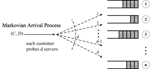
Figure 1: The supermarket model wherein each customer can probe $d$ servers

The following lemma, which is stated without proof, provides an intuitively sufficient condition under which the supermarket model is stable. Note that this proof can be given by a simple comparison argument with the queueing system in which each customer queues at a random server (i.e., where $d=1$). When $d=1$, each server acts like a MAP/PH/1 queue which is stable if $\rho=\lambda/\mu<1$, see chapter 5 in Neuts [37]. The comparison argument is similar to those in Winston [45] and Weber [44], thus we can obtain two useful results: (1) the shortest queue is optimal due to the assumptions on MAPs and PH service times; and (2) the size of the longest queue in the supermarket model is stochastically dominated by the size of the longest queue in a set of $n$ independent MAP/PH/1 queues.

Lemma 1

The supermarket model with MAPs and PH service times is stable if $\rho=\lambda/\mu<1.$

We define $n_{k}^{\left(i,j\right)}\left(t\right)$ as the number of queues with at least $k$ customers who include the customer in service, the MAP in phase $i$ and the PH service time in phase $j$ at time $t\geq 0$. Clearly, $0\leq n_{k}^{\left(i,j\right)}\left(t\right)\leq n$ for $1\leq i\leq m_{A}$, $1\leq j\leq m_{B}$ and $k\geq 0$. Let

$$x_{n}^{\left(i\right)}\left(0,t\right)=\frac{n_{0}^{\left(i\right)}\left(t\right)}{n}$$

and for $k\geq 1$

$$x_{n}^{\left(i,j\right)}\left(k,t\right)=\frac{n_{k}^{\left(i,j\right)}\left(t\right)}{n},$$

which is the fraction of queues with at least $k$ customers, the MAP in phase $i$ and the PH service time in phase $j$ at time $t\geq 0$. Using the lexicographic order we write

$$X_{n}\left(0,t\right)=\left(x_{n}^{\left(1\right)}\left(0,t\right),x_{n}^{\left(2\right)}\left(0,t\right),\ldots,x_{n}^{\left(m_{A}\right)}\left(0,t\right)\right)$$

and for $k\geq 1$

$$X_{n}\left(k,t\right)= (x_{n}^{\left(1,1\right)}\left(k,t\right),x_{n}^{\left(1,2\right)}\left(k,t\right),\ldots,x_{n}^{\left(1,m_{B}\right)}\left(k,t\right);\ldots;$$

$$x_{n}^{\left(m_{A},1\right)}\left(k,t\right),x_{n}^{\left(m_{A},2\right)}\left(k,t\right),\ldots,x_{n}^{\left(m_{A},m_{B}\right)}\left(k,t\right)),$$

$$X_{n}\left(t\right)=\left(X_{n}\left(0,t\right),X_{n}\left(1,t\right),X_{n}\left(2,t\right),\ldots\right).$$

The state of the supermarket model may be described by the vector $X_{n}\left(t\right)$ for $t\geq 0$. Since the arrival process to the queueing system is a MAP and the service time of each customer is of phase type, the stochastic process $\left\{X_{n}\left(t\right),t\geq 0\right\}$ describing the state of the supermarket model is a Markov process whose state space is given by

$$\Omega_{n}= \{\left(g_{n}^{\left(0\right)},g_{n}^{\left(1\right)},g_{n}^{\left(2\right)}\ldots\right):g_{n}^{\left(0\right)}\text{ is a probability vector, }g_{n}^{\left(k-1\right)}\geq g_{n}^{\left(k\right)}\geq 0$$

$$\text{ for }k\geq 2\text{,}\text{ and }ng_{n}^{\left(l\right)}\text{ is a vector of nonnegative integers for }l\geq 0\}.$$

Let

$$s_{0}^{\left(i\right)}\left(n,t\right)=E\left[x_{0}^{\left(i\right)}\left(n,t\right)\right]$$

and $k\geq 1$

$$s_{k}^{\left(i,j\right)}\left(n,t\right)=E\left[x_{k}^{\left(i,j\right)}\left(n,t\right)\right].$$

Using the lexicographic order we write

$$S_{0}\left(n,t\right)=\left(s_{0}^{\left(1\right)}\left(n,t\right),s_{0}^{\left(2\right)}\left(n,t\right),\ldots,s_{0}^{\left(m_{A}\right)}\left(n,t\right)\right)$$

and for $k\geq 1$

$$S_{k}\left(n,t\right)= (s_{k}^{\left(1,1\right)}\left(n,t\right),s_{k}^{\left(1,2\right)}\left(n,t\right),\ldots,s_{k}^{\left(1,m_{B}\right)}\left(n,t\right);\ldots;$$

$$s_{k}^{\left(m_{A},1\right)}\left(n,t\right),s_{k}^{\left(m_{A},2\right)}\left(n,t\right),\ldots,s_{k}^{\left(m_{A},m_{B}\right)}\left(n,t\right)),$$

$$S\left(n,t\right)=\left(S_{0}\left(n,t\right),S_{1}\left(n,t\right),S_{2}\left(n,t\right),\ldots\right).$$

As shown in Martin and Suhov [25] and Luczak and McDiarmid [21], the Markov process $\left\{X_{n}\left(t\right),t\geq 0\right\}$ is asymptotically deterministic as $n\rightarrow\infty$. Thus the limits $\lim_{n\rightarrow\infty}E\left[x_{0}^{\left(i\right)}\left(n,t\right)\right]$ and $\lim_{n\rightarrow\infty}E\left[x_{k}^{\left(i,j\right)}\left(n,t\right)\right]$ always exist by means of the law of large numbers. Based on this, we write

$$S_{0}\left(t\right)=\lim_{n\rightarrow\infty}S_{0}\left(n,t\right),$$

for $k\geq 1$

$$S_{k}\left(t\right)=\lim_{n\rightarrow\infty}S_{k}\left(n,t\right),$$

and

$$S\left(t\right)=\left(S_{0}\left(t\right),S_{1}\left(t\right),S_{2}\left(t\right),\ldots\right).$$

Note that $S_{0}\left(t\right)$ and $S_{k}\left(t\right)$ are two row vectors of order $m_{A}$ and $m_{A}m_{B}$, respectively. Let $X\left(t\right)=\lim_{n\rightarrow\infty}X_{n}\left(t\right)$. Then it is easy to see from the MAPs and the PH service times that $\left\{X\left(t\right),t\geq 0\right\}$ is also a Markov process whose state space is given by

$$\Omega=\left\{\left(g^{\left(0\right)},g^{\left(1\right)},g^{\left(2\right)},\ldots\right):g^{\left(0\right)}\text{ is a probability vector},g^{\left(k-1\right)}\geq g^{\left(k\right)}\geq 0\right\}.$$

If the initial distribution of the Markov process $\left\{X_{n}\left(t\right),t\geq 0\right\}$ approaches the Dirac delta-measure concentrated at a point $g\in$ $\Omega$, then the limit $X\left(t\right)=\lim_{n\rightarrow\infty}X_{n}\left(t\right)$ is concentrated on the trajectory $S_{g}=\left\{S\left(t\right):t\geq 0\right\}$. This indicates a law of large numbers for the time evolution of the fraction of queues of different lengths. Furthermore, the Markov process $\left\{X_{n}\left(t\right),t\geq 0\right\}$ converges weakly to the fraction vector $S\left(t\right)=\left(S_{0}\left(t\right),S_{1}\left(t\right),S_{2}\left(t\right),\ldots\right)$ as $n\rightarrow\infty$, or for a sufficiently small $\varepsilon>0$,

$$\lim_{n\rightarrow\infty}P\left\{||X_{n}\left(t\right)-S\left(t\right)||\geq\varepsilon\right\}=0,$$

where $||a||$ is the $L_{\infty}$-norm of vector $a$.

The following proposition shows that the sequence $\left\{S_{k}\left(t\right),k\geq 0\right\}$ is monotone decreasing, while its proof is easy by means of the definition of $S\left(t\right)$.

Proposition 1

For $1\leq k<l$

$$S_{l}\left(t\right)<S_{k}\left(t\right)$$

and

$$S_{l}\left(t\right)e<S_{k}\left(t\right)e<S_{0}\left(t\right)e=1.$$

In what follows we set up a system of differential vector equations satisfied by the fraction vector $S\left(t\right)$ by means of density dependent jump Markov processes.

We first provide an example to indicate how to derive the differential vector equations. Consider the supermarket model with $n$ servers, and determine the expected change in the number of queues with at least $k$ customers over a small time period of length d$t$. The probability vector that an arriving customer joins a queue of size $k-1$ during this time period is given by

$$\left[S_{k-1}^{\odot d}\left(n,t\right)\left(D\otimes I\right)+S_{k}^{\odot d}\left(n,t\right)\left(C\otimes I\right)\right]\cdot n\text{d}t,$$

since each arriving customer chooses $d\geq 1$ servers independently and uniformly at random from the $n$ servers, and waits for service at the server which currently contains the fewest number of customers. Similarly, the probability vector that a customer leaves a server queued by $k$ customers during this time period is given by

$$\left[S_{k}\left(n,t\right)\left(I\otimes T\right)+S_{k+1}\left(n,t\right)\left(I\otimes T^{0}\alpha\right)\right]\cdot n\text{d}t.$$

Therefore, we can obtain

$$\text{d}E\left[n_{k}\left(n,t\right)\right]= \left[S_{k-1}^{\odot d}\left(n,t\right)\left(D\otimes I\right)+S_{k}^{\odot d}\left(n,t\right)\left(C\otimes I\right)\right]\cdot n\text{d}t$$

$$+\left[S_{k}\left(n,t\right)\left(I\otimes T\right)+nS_{k+1}\left(n,t\right)\left(I\otimes T^{0}\alpha\right)\right]\cdot n\text{d}t,$$

which leads to

$$\frac{\text{d}S_{k}\left(n,t\right)}{\text{d}t}= S_{k-1}^{\odot d}\left(n,t\right)\left(D\otimes I\right)+S_{k}^{\odot d}\left(n,t\right)\left(C\otimes I\right)$$

$$+S_{k}\left(n,t\right)\left(I\otimes T\right)+S_{k+1}\left(n,t\right)\left(I\otimes T^{0}\alpha\right).$$ (1)

Using a similar analysis for Equation (1), we can obtain a system of differential vector equations for the fraction vector $S\left(n,t\right)=\left(S_{0}\left(n,t\right),S_{1}\left(n,t\right),S_{2}\left(n,t\right),\ldots\right)$ as follows:

$$S_{0}\left(n,t\right)e=1,$$ (2)

$$\frac{\mathtt{d}}{\text{d}t}S_{0}\left(n,t\right)=S_{0}^{\odot d}\left(n,t\right)C+S_{1}\left(n,t\right)\left(I\otimes T^{0}\right),$$ (3)

$$\frac{\mathtt{d}}{\text{d}t}S_{1}\left(n,t\right)= S_{0}^{\odot d}\left(n,t\right)\left(D\otimes\alpha\right)+S_{1}^{\odot d}\left(n,t\right)\left(C\otimes I\right)$$

$$+S_{1}\left(n,t\right)\left(I\otimes T\right)+S_{2}\left(n,t\right)\left(I\otimes T^{0}\alpha\right),$$ (4)

and for $k\geq 2$

$$\frac{\text{d}S_{k}\left(n,t\right)}{\text{d}t}= S_{k-1}^{\odot d}\left(n,t\right)\left(D\otimes I\right)+S_{k}^{\odot d}\left(n,t\right)\left(C\otimes I\right)$$

$$+S_{k}\left(n,t\right)\left(I\otimes T\right)+S_{k+1}\left(n,t\right)\left(I\otimes T^{0}\alpha\right).$$ (5)

Noting that the limit $\lim_{n\rightarrow\infty}S_{k}\left(n,t\right)$ exists for $k\geq 0$ and taking $n\rightarrow\infty$ in the both sides of the system of differential vector equations (2) to (5), we can easily obtain a system of differential vector equations for the fraction vector $S\left(t\right)=\left(S_{0}\left(t\right),S_{1}\left(t\right),S_{2}\left(t\right),\ldots\right)$ as follows:

$$S_{0}\left(t\right)e=1,$$ (6)

$$\frac{\mathtt{d}}{\text{d}t}S_{0}\left(t\right)=S_{0}^{\odot d}\left(t\right)C+S_{1}\left(t\right)\left(I\otimes T^{0}\right),$$ (7)

$$\frac{\mathtt{d}}{\text{d}t}S_{1}\left(t\right)= S_{0}^{\odot d}\left(t\right)\left(D\otimes\alpha\right)+S_{1}^{\odot d}\left(t\right)\left(C\otimes I\right)$$

$$+S_{1}\left(t\right)\left(I\otimes T\right)+S_{2}\left(t\right)\left(I\otimes T^{0}\alpha\right),$$ (8)

and for $k\geq 2$,

$$\frac{\text{d}S_{k}\left(t\right)}{\text{d}t}= S_{k-1}^{\odot d}\left(t\right)\left(D\otimes I\right)+S_{k}^{\odot d}\left(t\right)\left(C\otimes I\right)$$

$$+S_{k}\left(t\right)\left(I\otimes T\right)+S_{k+1}\left(t\right)\left(I\otimes T^{0}\alpha\right).$$ (9)

Remark 1

(a) For the supermarket model, many papers, such as Mitzenmacher [26] and Luczak and McDiarmid [21], assumed that the arrival process is Poisson with rate $n\lambda$. As a direct generalization of the Poisson arrivals with rate $n\lambda$, this paper uses a MAP with an irreducible matrix descriptor $\left(nC,nD\right)$ of size $m_{A}$ whose stationary arrival rate is given by $n\lambda=n\gamma De$.

(b) When there are $n$ servers in the supermarket model, we may use a more general MAP with an irreducible matrix descriptor $\left(C_{n},D_{n}\right)$ of size $m_{A}$, where

$$\lim_{n\rightarrow\infty}\frac{C_{n}}{n}=C,\text{ \ }\lim_{n\rightarrow\infty}\frac{D_{n}}{n}=D,$$

and $\left(C,D\right)$ is also the irreducible matrix descriptor of a MAP. It is easy to see from the above analysis that we can also obtain the system of differential vector equations (6) to (9) with respect to the more general MAP.

3 Doubly Exponential Solution

In this section, we provide a novel matrix-analytic approach for computing the fixed point of the system of differential vector equations (6) to (9), and give a closed-form solution with a doubly exponential structure to the fixed point.

A row vector $\pi=\left(\pi_{0},\pi_{1},\pi_{2},\ldots\right)$ is called a fixed point of the fraction vector $S\left(t\right)$ if $\lim_{t\rightarrow+\infty}S\left(t\right)=\pi$. In this case, it is easy to see that

$$\lim_{t\rightarrow+\infty}\left[\frac{\mathtt{d}}{\text{d}t}S\left(t\right)\right]=0.$$

Therefore, as $t\rightarrow+\infty$ the system of differential vector equations (6) to (9) can be simplified as a system of nonlinear equations as follows:

$$\pi_{0}e=1,$$ (10)

$$\pi_{0}^{\odot d}C++\pi_{1}\left(I\otimes T^{0}\right)=0,$$ (11)

$$\pi_{0}^{\odot d}\left(D\otimes\alpha\right)+\pi_{1}^{\odot d}\left(C\otimes I\right)+\pi_{1}\left(I\otimes T\right)+\pi_{2}\left(I\otimes T^{0}\alpha\right)=0,$$ (12)

and for $k\geq 2$,

$$\pi_{k-1}^{\odot d}\left(D\otimes I\right)+\pi_{k}^{\odot d}\left(C\otimes I\right)+\pi_{k}\left(I\otimes T\right)+\pi_{k+1}\left(I\otimes T^{0}\alpha\right)=0.$$ (13)

It is very challenging to solve the system of nonlinear equations (10) to (13). Here, our goal is to derive a closed-form solution with a doubly exponential structure to the fixed point $\pi=(\pi_{0},\pi_{1},\pi_{2},...)$ through a novel matrix-analytic approach.

It follows from Equations (12) and (13) that

$$\left(\pi_{1}^{\odot d},\pi_{2}^{\odot d},\pi_{3}^{\odot d},\ldots\right)\left(\begin{array}[c]{ccccc}C\otimes I&D\otimes I&&&\\ &C\otimes I&D\otimes I&&\\ &&C\otimes I&D\otimes I&\\ &&&\ddots&\ddots\end{array}\right)$$ (18)

$$+ \left(\pi_{1},\pi_{2},\pi_{3},\ldots\right)\left(\begin{array}[c]{cccc}I\otimes T&&&\\ I\otimes T^{0}\alpha&I\otimes T&&\\ &I\otimes T^{0}\alpha&I\otimes T&\\ &&\ddots&\ddots\end{array}\right)$$ (23)

$$=-\left(\pi_{0}^{\odot d}\left(D\otimes\alpha\right),0,0,\ldots\right).$$ (24)

Let

$$A=\left(\begin{array}[c]{cccc}I\otimes T&&&\\ I\otimes T^{0}\alpha&I\otimes T&&\\ &I\otimes T^{0}\alpha&I\otimes T&\\ &&\ddots&\ddots\end{array}\right).$$

Then it is easy to check that the matrix $A$ is invertible, and

$$-A^{-1}=\left(\begin{array}[c]{ccccc}I\otimes\left(-T\right)^{-1}&&&&\\ I\otimes\left[e\alpha\left(-T\right)^{-1}\right]&I\otimes\left(-T\right)^{-1}&&&\\ I\otimes\left[e\alpha\left(-T\right)^{-1}\right]&I\otimes\left[e\alpha\left(-T\right)^{-1}\right]&I\otimes\left(-T\right)^{-1}&&\\ I\otimes\left[e\alpha\left(-T\right)^{-1}\right]&I\otimes\left[e\alpha\left(-T\right)^{-1}\right]&I\otimes\left[e\alpha\left(-T\right)^{-1}\right]&I\otimes\left(-T\right)^{-1}&\\ \vdots&\vdots&\vdots&\vdots&\ddots\end{array}\right),$$

$$\left(\begin{array}[c]{ccccc}C\otimes I&D\otimes I&&&\\ &C\otimes I&D\otimes I&&\\ &&C\otimes I&D\otimes I&\\ &&&\ddots&\ddots\end{array}\right)\left(-A^{-1}\right)=\left(\begin{array}[c]{ccccc}R&V&&&\\ W&R&V&&\\ W&W&R&V&\\ \vdots&\vdots&\vdots&\vdots&\ddots\end{array}\right),$$

and

$$\left(\pi_{0}^{\odot d}\left(D\otimes\alpha\right),0,0,\ldots\right)\left(-A^{-1}\right)=\left(\pi_{0}^{\odot d}D\otimes\left[\alpha\left(-T\right)^{-1}\right],0,0,\ldots\right),$$

where

$$V=D\otimes\left(-T\right)^{-1},$$

$$W=\left(C+D\right)\otimes\left[e\alpha\left(-T\right)^{-1}\right]$$

and

$$R=C\otimes\left(-T\right)^{-1}+D\otimes\left[e\alpha\left(-T\right)^{-1}\right].$$

Thus it follows from (24) that

$$\left(\pi_{1},\pi_{2},\pi_{3},\ldots\right)= \left(\pi_{1}^{\odot d},\pi_{2}^{\odot d},\pi_{3}^{\odot d},\ldots\right)\left(\begin{array}[c]{ccccc}R&V&&&\\ W&R&V&&\\ W&W&R&V&\\ \vdots&\vdots&\vdots&\vdots&\ddots\end{array}\right)$$ (29)

$$+\left(\pi_{0}^{\odot d}D\otimes\left[\alpha\left(-T\right)^{-1}\right],0,0,\ldots\right),$$ (30)

which leads to a new system of nonlinear equations as follows:

$$\pi_{1}=\pi_{0}^{\odot d}D\otimes\left[\alpha\left(-T\right)^{-1}\right]+\pi_{1}^{\odot d}R+\sum_{j=2}^{\infty}\pi_{j}^{\odot d}W$$ (31)

and for $k\geq 2$,

$$\pi_{k}=\pi_{k-1}^{\odot d}V+\pi_{k}^{\odot d}R+\sum_{j=k+1}^{\infty}\pi_{j}^{\odot d}W.$$ (32)

Now, we need to omit the two terms $\pi_{l}^{\odot d}R$ for $l\geq 1$ and $\sum_{j=k}^{\infty}\pi_{j}^{\odot d}W$ for $k\geq 2$ in Equations (31) and (32). Note that the Markov chain $C+D$ is positive recurrent, we assume that the system of nonlinear equations (31) and (32) has a closed-form solution

$$\pi_{0}=\theta\gamma^{\odot\frac{1}{d}}$$ (33)

and for $k\geq 1$

$$\pi_{k}=r\left(k\right)\left(\gamma^{\odot\frac{1}{d}}\otimes\alpha^{\odot\frac{1}{d}}\right),$$ (34)

where $\theta=1/\gamma^{\odot\frac{1}{d}}e$, and $r\left(k\right)$ is a positive constant for $k\geq 1$. Then it follows from (31), (32) and (34) that

$$r\left(1\right)\left(\gamma^{\odot\frac{1}{d}}\otimes\alpha^{\odot\frac{1}{d}}\right)= \pi_{0}^{\odot d}D\otimes\left[\alpha\left(-T\right)^{-1}\right]+r^{d}\left(1\right)\left(\gamma\otimes\alpha\right)R$$

$$+\sum_{j=2}^{\infty}r^{d}\left(j\right)\left(\gamma\otimes\alpha\right)W;$$ (35)

and for $k\geq 2$,

$$r\left(k\right)\left(\gamma^{\odot\frac{1}{d}}\otimes\alpha^{\odot\frac{1}{d}}\right)= r^{d}\left(k-1\right)\left(\gamma\otimes\alpha\right)V+r^{d}\left(k\right)\left(\gamma\otimes\alpha\right)R$$

$$+\sum_{j=k+1}^{\infty}r^{d}\left(j\right)\left(\gamma\otimes\alpha\right)W.$$ (36)

Note that

$$\left(\gamma\otimes\alpha\right)W =\left(\gamma\otimes\alpha\right)\left\{\left(C+D\right)\otimes\left[e\alpha\left(-T\right)^{-1}\right]\right\}$$

$$=\gamma\left(C+D\right)\otimes\alpha\left[e\alpha\left(-T\right)^{-1}\right]$$

and

$$\gamma\left(C+D\right)=0,$$

it is clear that

$$\left(\gamma\otimes\alpha\right)W=0.$$

Similarly, we can compute

$$\left(\gamma\otimes\alpha\right)R =\left(\gamma\otimes\alpha\right)\left\{C\otimes\left(-T\right)^{-1}+D\otimes\left[e\alpha\left(-T\right)^{-1}\right]\right\}$$

$$=\gamma\left(C+D\right)\otimes\alpha\left(-T\right)^{-1}=0.$$

It follows from (35) and (36) that

$$\pi_{1}=\pi_{0}^{\odot d}D\otimes\left[\alpha\left(-T\right)^{-1}\right]$$ (37)

or

$$r\left(1\right)\left(\gamma^{\odot\frac{1}{d}}\otimes\alpha^{\odot\frac{1}{d}}\right)=\pi_{0}^{\odot d}D\otimes\left[\alpha\left(-T\right)^{-1}\right];$$ (38)

and for $k\geq 2$

$$\pi_{k}=\pi_{k-1}^{\odot d}\left(D\otimes\left(-T\right)^{-1}\right)$$ (39)

or

$$r\left(k\right)\left(\gamma^{\odot\frac{1}{d}}\otimes\alpha^{\odot\frac{1}{d}}\right)=r^{d}\left(k-1\right)\left(\gamma\otimes\alpha\right)\left(D\otimes\left(-T\right)^{-1}\right).$$ (40)

Let $\omega=1/\alpha^{\odot\frac{1}{d}}e$. Then $0<\theta,\omega<1$ due to $\gamma^{\odot\frac{1}{d}}e>1$ and $\alpha^{\odot\frac{1}{d}}e>1$. Note that $\pi_{0}=\theta\gamma^{\odot\frac{1}{d}}$, $\lambda=\gamma De$, $1/\mu=\alpha\left(-T\right)^{-1}e$ and $\rho=\lambda/\mu$, it follows from (38) and (40) that

$$r\left(1\right)=\theta^{d}\left(\theta\omega\rho\right)$$ (41)

and for $k\geq 2$

$$r\left(k\right) =r^{d}\left(k-1\right)\theta\omega\rho$$

$$=\left[r\left(1\right)\right]^{d^{k-1}}\left(\theta\omega\rho\right)^{d^{k-2}+d^{k-3}+\cdots+1}$$

$$=\theta^{d^{k}}\left(\theta\omega\rho\right)^{d^{k-1}+d^{k-2}+\cdots+1}$$

$$=\theta^{d^{k}}\left(\theta\omega\rho\right)^{\frac{d^{k}-1}{d-1}}.$$ (42)

It is easy to see from (33), (34) and (42) that

$$\pi_{0}=\theta\cdot\gamma^{\odot\frac{1}{d}}$$ (43)

and for $k\geq 1$

$$\pi_{k}=\theta^{d^{k}}\left(\theta\omega\rho\right)^{\frac{d^{k}-1}{d-1}}\cdot\gamma^{\odot\frac{1}{d}}\otimes\alpha^{\odot\frac{1}{d}}.$$ (44)

Now, we use (43) and (44) to check Equations (11) and (37) that

$$\left\{\begin{array}[c]{l}\pi_{0}^{\odot d}C+\pi_{1}\left(I\otimes T^{0}\right)=0,\\ \pi_{1}=\pi_{0}^{\odot d}D\otimes\left[\alpha\left(-T\right)^{-1}\right],\end{array}\right.$$

which leads to

$$\pi_{0}^{\odot d}\left(C+D\right)=0.$$ (45)

Obviously, $\pi_{0}=\theta\cdot\gamma^{\odot\frac{1}{d}}$ is a non-zero nonnegative solution to Equation (45), and $\pi_{0}e=1$.

Summarizing the above analysis, the following theorem describes a closed-form solution with a doubly exponential structure to the fixed point.

Theorem 1

The fixed point $\pi=\left(\pi_{0},\pi_{1},\pi_{2},\ldots\right)$ is given by

$$\pi_{0}=\theta\cdot\gamma^{\odot\frac{1}{d}},$$

and for $k\geq 1,$

$$\pi_{k}=\theta^{d^{k}}\left(\theta\omega\rho\right)^{\frac{d^{k}-1}{d-1}}\cdot\gamma^{\odot\frac{1}{d}}\otimes\alpha^{\odot\frac{1}{d}}.$$

The following corollary indicates that the fixed point can be decomposed into the product of two factors inflecting arrival information and service information. Based on this, it is easy to see the role played by the arrival and service processes in the fixed point.

Corollary 2

The fixed point $\pi=\left(\pi_{0},\pi_{1},\pi_{2},\ldots\right)$ can be decomposed into the product of two factors inflecting arrival information and service information

$$\pi_{k}=\left\{\theta^{\frac{d^{k+1}-1}{d-1}}\lambda^{\frac{d^{k}-1}{d-1}}\cdot\gamma^{\odot\frac{1}{d}}\right\}\otimes\left\{\left(\frac{\omega}{\mu}\right)^{\frac{d^{k}-1}{d-1}}\cdot\alpha^{\odot\frac{1}{d}}\right\},\text{ \ }k\geq 0.$$

Remark 2

We consider a supermarket model with Poisson arrivals with rate $\lambda$ and exponential service times with rate $\mu$, which has been extensively analyzed in the literature. Obviously, $\pi_{0}=1$. It follows from (24) that

$$\left(\pi_{1}^{\odot d},\pi_{2}^{\odot d},\pi_{3}^{\odot d},\ldots\right)\left(\begin{array}[c]{ccccc}-\lambda&\lambda&&&\\ &-\lambda&\lambda&&\\ &&-\lambda&\lambda&\\ &&&\ddots&\ddots\end{array}\right)\newline$$

$$+ \left(\pi_{1},\pi_{2},\pi_{3},\ldots\right)\left(\begin{array}[c]{cccc}-\mu&&&\\ \mu&-\mu&&\\ &\mu&-\mu&\\ &&\ddots&\ddots\end{array}\right)=-\left(\lambda,0,0,\ldots\right),$$

which leads to

$$\left(\pi_{1},\pi_{2},\pi_{3},\ldots\right)=\left(\pi_{1}^{\odot d},\pi_{2}^{\odot d},\pi_{3}^{\odot d},\ldots\right)\left(\begin{array}[c]{ccccc}0&\rho&&&\\ &0&\rho&&\\ &&0&\rho&\\ &&&\ddots&\ddots\end{array}\right)+\left(\rho,0,0,\ldots\right).$$

Thus we obtain

$$\pi_{1}=\rho$$

and for $k\geq 2$,

$$\pi_{k}=\rho\pi_{k-1}^{\odot d}=\rho^{d^{k-1}+d^{k-2}+\cdots+1}=\rho^{\frac{d^{k}-1}{d-1}},$$

which is the same as Lemma 3.2 in Mitzenmacher [27].

Based on Theorem 1, we now compute the expected sojourn time $T_{d}$ that a tagged arriving customer spends in the supermarket model. For the PH service time $X$ with an irreducible representation $\left(\alpha,T\right)$, the residual time $X_{R}$ of $X$ is also of phase type with an irreducible representation $\left(\tau,T\right)$, where $\tau$ is the stationary probability vector of the Markov chain $T+T^{0}\alpha$. Thus, we have

$$E\left[X\right]=\alpha\left(-T\right)^{-1}e=\frac{1}{\mu},\text{ \ }E\left[X_{R}\right]=\tau\left(-T\right)^{-1}e.$$

For the PH service times, a tagged arriving customer is the $k$th customer in the corresponding queue with probability $\pi_{k-1}^{\odot d}e-\pi_{k}^{\odot d}e$. Thus it is easy to see that the expected sojourn time of the tagged arriving customer is given by

$$E\left[T_{d}\right] =\left(\pi_{0}^{\odot d}e-\pi_{1}^{\odot d}e\right)E\left[X\right]+\sum_{k=1}^{\infty}\left(\pi_{k}^{\odot d}e-\pi_{k+1}^{\odot d}e\right)\left[E\left[X_{R}\right]+kE\left[X\right]\right]$$

$$=\left\{E\left[X_{R}\right]-E\left[X\right]\right\}\pi_{1}^{\odot d}e+E\left[X\right]\sum_{k=0}^{\infty}\pi_{k}^{\odot d}e$$

$$=\theta^{d^{2}}\left(\theta\omega\rho\right)^{d}\left(\tau-\alpha\right)\left(-T\right)^{-1}e+\frac{1}{\mu}\sum_{k=0}^{\infty}\theta^{d^{k+1}}\left(\theta\omega\rho\right)^{\frac{d^{k+1}-d}{d-1}}.$$

When the arrival process and the service time distribution are Poisson and exponential, respectively, it is clear that $\alpha=\tau=1$ and $\theta=\omega=1$, thus we have

$$E\left[T_{d}\right]=\frac{1}{\mu}\sum_{k=0}^{\infty}\rho^{\frac{d^{k+1}-d}{d-1}},$$

which is the same as Corollary 3.8 in Mitzenmacher [27].

In what follows we provide an example to indicate how the expected sojourn time $E[T_{d}]$ depends on the choice number $d$. We assume that $m=2$ and

$$C=\left(\begin{array}[c]{cc}-10&7\\ 4&-9\end{array}\right),\ \ D=\left(\begin{array}[c]{cc}1&2\\ 3&2\end{array}\right),$$

and the service times are exponential with service rate $\mu=5,10,20$, respectively. It is seen from Figure 2 that the expected sojourn time $E[T_{d}]$ decreases very fast as the choice number $d$ increases.

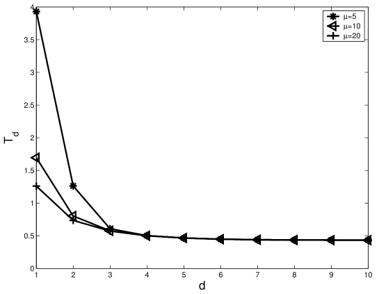
Figure 2: $E[T_{d}]$ vs $d$ for the MAP

4 An Important Observation

In this section, we analyze a special supermarket model with Poisson arrivals an PH service times, and obtain two different doubly exponential solutions to the fixed point. Based on this, we give an important observation, namely that the doubly exponential solution to the fixed point is not always unique for more general supermarket models.

When the arrival process is Poisson, it follows from (10) to (13) that

$$\pi_{0}=1,$$ (46)

$$-\lambda+\pi_{1}T^{0}=0,$$ (47)

$$\lambda\alpha-\lambda\pi_{1}^{\odot d}+\pi_{1}T+\pi_{2}T^{0}\alpha=0,$$ (48)

and for $k\geq 2$,

$$\lambda\pi_{k-1}^{\odot d}\left(t\right)-\lambda\pi_{k}^{\odot d}\left(t\right)+\pi_{k}\left(t\right)T+\pi_{k+1}\left(t\right)T^{0}\alpha=0.$$ (49)

For the system of nonlinear equations (46) to (49), we can provide two different doubly exponential solutions to the fixed point $\pi=\left(\pi_{0},\pi_{1},\pi_{2},\ldots\right)$.

4.1 The first doubly exponential solution

The first doubly exponential solution has been given in Section 3. Here, we simply list the crucial derivations for the special supermarket model.

It follows from (24) that

$$\left(\pi_{1}^{\odot d},\pi_{2}^{\odot d},\pi_{3}^{\odot d},\ldots\right)\left(\begin{array}[c]{ccccc}-\lambda&\lambda&&&\\ &-\lambda&\lambda&&\\ &&-\lambda&\lambda&\\ &&&\ddots&\ddots\end{array}\right)+\left(\pi_{1},\pi_{2},\pi_{3},\ldots\right)\left(\begin{array}[c]{cccc}T&&&\\ T^{0}\alpha&T&&\\ &T^{0}\alpha&T&\\ &&\ddots&\ddots\end{array}\right)$$

$$=-\left(\lambda\alpha,0,0,\ldots\right),$$

which leads to

$$\left(\pi_{1},\pi_{2},\pi_{3},\ldots\right)= \left(\pi_{1}^{\odot d},\pi_{2}^{\odot d},\pi_{3}^{\odot d},\ldots\right)\left(\begin{array}[c]{ccccc}R&V&&&\\ &R&V&&\\ &&R&V&\\ &&&\ddots&\ddots\end{array}\right)$$

$$+\left(\lambda\alpha\left(-T\right)^{-1},0,0,\ldots\right),$$

where

$$V=\lambda\left(-T\right)^{-1}$$

and

$$R=\lambda\left(-I+e\alpha\right)\left(-T\right)^{-1}.$$

Thus we obtain

$$\pi_{1}=\lambda\alpha\left(-T\right)^{-1}+\pi_{1}^{\odot d}\left[\lambda\left(-I+e\alpha\right)\left(-T\right)^{-1}\right]$$ (50)

and for $k\geq 2$

$$\pi_{k}=\pi_{k-1}^{\odot d}\left[\lambda\left(-T\right)^{-1}\right]+\pi_{k}^{\odot d}\left[\lambda\left(-I+e\alpha\right)\left(-T\right)^{-1}\right].$$ (51)

To omit the term $\pi_{k}^{\odot d}\left[\lambda\left(-I+e\alpha\right)\left(-T\right)^{-1}\right]$ for $k\geq 1$, we assume that $\left\{\pi_{k},k\geq 1\right\}$ has the following expression

$$\pi_{k}=r\left(k\right)\alpha^{\odot\frac{1}{d}}.$$

In this case, we have

$$\pi_{k}^{\odot d}\left[\lambda\left(-I+e\alpha\right)\left(-T\right)^{-1}\right]=r^{d}\left(k\right)\alpha\left[\lambda\left(-I+e\alpha\right)\left(-T\right)^{-1}\right]=0,$$

thus it follows from (50) and (51) that

$$\pi_{1}=\lambda\alpha\left(-T\right)^{-1}$$ (52)

and for $k\geq 2$

$$\pi_{k}=\pi_{k-1}^{\odot d}\left[\lambda\left(-T\right)^{-1}\right].$$ (53)

It follows from (52) that

$$r\left(1\right)\alpha^{\odot\frac{1}{d}}=\lambda\alpha\left(-T\right)^{-1},$$

which follows that

$$r\left(1\right)=\omega\rho.$$

It follows from (53) that

$$r\left(k\right)\alpha^{\odot\frac{1}{d}}=r^{d}\left(k-1\right)\alpha\left[\lambda\left(-T\right)^{-1}\right]$$

which follows that

$$r\left(k\right)=r^{d}\left(k-1\right)\omega\rho=\left(\omega\rho\right)^{\frac{d^{k}-1}{d-1}}.$$

Therefore, we can obtain

$$\pi_{0}=1$$

and for $k\geq 1$

$$\pi_{k}=\left(\omega\rho\right)^{\frac{d^{k}-1}{d-1}}\cdot\alpha^{\odot\frac{1}{d}}.$$ (54)

4.2 The second doubly exponential solution

The second doubly exponential solution was given in Li, Lui and Wang [19], thus we provide some crucial computational steps.

It follows from (47) that

$$\pi_{1}T^{0}=\lambda.$$ (55)

To solve Equation (55), we denote by $\tau$ the stationary probability vector of the irreducible Markov chain $T+T^{0}\alpha$. Obviously, we have

$$\tau T^{0}=\mu,$$

$$\frac{\lambda}{\mu}\tau T^{0}=\lambda.$$ (56)

Thus, we obtain

$$\pi_{1}=\frac{\lambda}{\mu}\tau=\rho\cdot\tau.$$

Using $\pi_{0}=1$ and $\pi_{1}=\rho\cdot\tau$, it follows from Equation (48) that

$$\lambda\alpha-\lambda\rho^{d}\cdot\tau^{\odot d}+\rho\cdot\tau T+\pi_{2}T^{0}\alpha=0,$$

which leads to

$$\lambda-\lambda\rho^{d}\cdot\tau^{\odot d}e+\rho\cdot\tau Te+\pi_{2}T^{0}=0.$$

Note that $\tau Te=-\mu$ and $\rho=\lambda/\mu$, we obtain

$$\pi_{2}T^{0}=\lambda\rho^{d}\tau^{\odot d}e.$$

Let $\psi=\tau^{\odot d}e$. Then it is easy to see that $\psi\in\left(0,1\right)$, and

$$\pi_{2}T^{0}=\lambda\psi\rho^{d}.$$

Using similar analysis on Equation (55), we have

$$\pi_{2}=\frac{\lambda\psi\rho^{d}}{\mu}\tau=\psi\rho^{d+1}\cdot\tau.$$

Based on $\pi_{1}=\rho\cdot\tau$ and $\pi_{2}=\psi\rho^{d+1}\cdot\tau$, it follows from Equation (49) that for $k=2$,

$$\lambda\rho^{d}\cdot\tau^{\odot d}-\lambda\psi^{d}\rho^{d^{2}+d}\cdot\tau^{\odot d}+\psi\rho^{d+1}\cdot\tau T+\pi_{3}T^{0}\alpha=0,$$

which leads to

$$\lambda\psi\rho^{d}-\lambda\psi^{d+1}\rho^{d^{2}+d}+\psi\rho^{d+1}\cdot\tau Te+\pi_{3}T^{0}=0,$$

thus we obtain

$$\pi_{3}T^{0}=\lambda\psi^{d+1}\rho^{d^{2}+d}.$$

Using a similar analysis on Equation (55), we have

$$\pi_{3}=\frac{\lambda\psi^{d+1}\rho^{d^{2}+d}}{\mu}\tau=\psi^{d+1}\rho^{d^{2}+d+1}\cdot\tau.$$

Now, we assume that $\pi_{k}=\psi^{\frac{d^{k-1}-1}{d-1}}\rho^{\frac{d^{k}-1}{d-1}}\cdot\tau$ is correct for the cases with $l=k$. Then for $l=k+1$ we have

$$\lambda \psi^{d^{k-2}+d^{k-3}+\cdots+d}\rho^{d^{k-1}+d^{k-2}+\cdots+d}\cdot\tau^{\odot d}-\lambda\psi^{d^{k-1}+d^{k-2}+\cdots+d}\rho^{d^{k}+d^{k-1}+\cdots+d}\cdot\tau^{\odot d}$$

$$+\psi^{d^{k-2}+d^{k-3}+\cdots+1}\rho^{d^{k-1}+d^{k-2}+\cdots+1}\cdot\tau T+\pi_{k+1}T^{0}\alpha=0,$$

which leads to

$$\lambda \psi^{d^{k-2}+d^{k-3}+\cdots+d+1}\rho^{d^{k-1}+d^{k-2}+\cdots+d}-\lambda\psi^{d^{k-1}+d^{k-2}+\cdots+d+1}\rho^{d^{k}+d^{k-1}+\cdots+d}$$

$$+\psi^{d^{k-2}+d^{k-3}+\cdots+1}\rho^{d^{k-1}+d^{k-2}+\cdots+1}\cdot\tau Te+\pi_{k+1}T^{0}=0,$$

thus we obtain

$$\pi_{k+1}T^{0}=\lambda\psi^{d^{k-1}+d^{k-2}+\cdots+d+1}\rho^{d^{k}+d^{k-1}+\cdots+d}.$$

By a similar analysis to (55) and (56), we have

$$\pi_{k+1} =\frac{\lambda\psi^{d^{k-1}+d^{k-2}+\cdots+d+1}\rho^{d^{k}+d^{k-1}+\cdots+d}}{\mu}\tau$$

$$=\psi^{d^{k-1}+d^{k-2}+\cdots+d+1}\rho^{d^{k}+d^{k-1}+\cdots+d+1}\cdot\tau.$$

Therefore, by induction we can obtain

$$\pi_{0}=1,$$

and for $k\geq 1$

$$\pi_{k}=\psi^{\frac{d^{k-1}-1}{d-1}}\rho^{\frac{d^{k}-1}{d-1}}\cdot\tau.$$ (57)

4.3 An important observation

Now, we have given two expressions (54) and (57) for the fixed point. In what follows we provide some examples to indicate that the two expressions may be different from each other.

Example one: When the PH service time is exponential, it is easy to see that $\alpha=\tau=1$, which leads to that $\omega=\psi=1$. Thus the fixed point is given by

$$\pi_{k}=\rho^{\frac{d^{k}-1}{d-1}},k\geq 1.$$

In this case, (54) is the same as (57).

Example two: When the service time is an $m$-order Erlang distribution with an irreducible representation $(\alpha,T)$, where

$$\alpha=\left(1,0,\ldots,0\right)$$

and

$$T=\left(\begin{array}[c]{ccccc}-\eta&\eta&&&\\ &-\eta&\eta&&\\ &&\ddots&\ddots&\\ &&&-\eta&\eta\\ &&&&-\eta\end{array}\right),\text{ \ \ }T^{0}=\left(\begin{array}[c]{c}0\\ 0\\ \vdots\\ 0\\ \eta\end{array}\right).$$

We have

$$\alpha^{\odot\frac{1}{d}}=\left(1,0,\ldots,0\right)$$

and

$$\omega=\frac{1}{\alpha^{\odot\frac{1}{d}}e}=1.$$

Thus the first doubly exponential solution is given by

$$\pi_{k}^{\left(\text{F}\right)}=\rho^{\frac{d^{k}-1}{d-1}}\cdot\left(1,0,\ldots,0\right),\text{ \ }k\geq 1.$$ (58)

It is clear that

$$T+T^{0}\alpha=\left(\begin{array}[c]{ccccc}-\eta&\eta&&&\\ &-\eta&\eta&&\\ &&\ddots&\ddots&\\ &&&-\eta&\eta\\ \eta&&&&-\eta\end{array}\right),$$

which leads to the stationary probability vector of the Markov chain $T+T^{0}\alpha$ as follows:

$$\tau=\left(\frac{1}{m},\frac{1}{m},\ldots,\frac{1}{m}\right),$$

$$\mu=\tau T^{0}=\frac{\eta}{m},$$

$$\rho=\frac{\lambda}{\mu}=\frac{m\lambda}{\eta}$$

and

$$\psi=m\left(\frac{1}{m}\right)^{d}=m^{1-d}.$$

Thus the second doubly exponential solution is given by

$$\pi_{k}^{\left(\text{S}\right)} =\psi^{\frac{d^{k-1}-1}{d-1}}\rho^{\frac{d^{k}-1}{d-1}}\left(\frac{1}{m},\frac{1}{m},\ldots,\frac{1}{m}\right)$$

$$=\rho^{\frac{d^{k}-1}{d-1}}\cdot\left(m^{-d^{k-1}},m^{-d^{k-1}},\ldots,m^{-d^{k-1}}\right),\text{ \ }k\geq 1.$$ (59)

It is clear that (58) and (59) are different from each other for $k,m,d\geq 2$, and

$$\frac{\pi_{k}^{\left(\text{F}\right)}e}{\pi_{k}^{\left(\text{S}\right)}e}=m^{d^{k-1}-1}.$$

It is clear that $\pi_{k}^{\left(\text{F}\right)}e\neq\pi_{k}^{\left(\text{S}\right)}e$ for $k,m,d\geq 2$.

Remark 3

For the supermarket model with Poisson arrivals and PH service times, we have obtained two different doubly exponential solutions to the fixed point. It is interesting but difficult to be able to find another new doubly exponential solution to the fixed point. Furthermore, we believe that it is an open problem how to give all doubly exponential solutions to the fixed point for more general supermarket models.

5 Exponential Convergence

In this section, we provide an upper bound for the current location $S\left(t\right)$ of the supermarket model, and study exponential convergence of the current location $S\left(t\right)$ to its fixed point $\pi$.

For the supermarket model, the initial point $S\left(0\right)$ can affect the current location $S\left(t\right)$ for each $t>0$, since the arrival and service processes are under a unified structure through a sample path comparison. To explain this, it is necessary to provide some notation for comparison of two vectors. Let $a=\left(a_{1},a_{2},a_{3},\ldots\right)$ and $b=\left(b_{1},b_{2},b_{3},\ldots\right)$. We write $a\prec b$ if $a_{k}<b_{k}$ for some $k\geq 1$ and $a_{l}\leq b_{l}$ for $l\neq k,l\geq 1$; and $a\preceq b$ if $a_{k}\leq b_{k}$ for all $k\geq 1$.

Now, we can easily obtain the following useful proposition, while the proof is clear by means of a sample path analysis, and thus is omitted here.

Proposition 2

If $S\left(0\right)\preceq\widetilde{S}\left(0\right)$, then $S\left(t\right)\preceq\widetilde{S}\left(t\right)$ for $t>0$.

Based on Proposition 2, the following theorem shows that the fixed point $\pi$ is an upper bound of the current location $S\left(t\right)$ for all $t\geq 0$.

Theorem 3

For the supermarket model, if there exists some $k$ such that $S_{k}\left(0\right)=0$, then the sequence $\left\{S_{k}\left(t\right)\right\}$ for all $t\geq 0$ has an upper bound sequence $\left\{\pi_{k}\right\}$ which decreases doubly exponentially, that is, $S\left(t\right)\preceq\pi$ for all $t\geq 0$.

Proof:  Let

$$\widetilde{S}_{k}\left(0\right)=\pi_{k},\text{ \ }k\geq 0.$$

Then for each $k\geq 0$, $\widetilde{S}_{k}\left(t\right)=\widetilde{S}_{k}\left(0\right)=\pi_{k}$ for all $t\geq 0$, since

$$\widetilde{S}\left(0\right)=\left(\widetilde{S}_{0}\left(0\right),\widetilde{S}_{1}\left(0\right),\widetilde{S}_{2}\left(0\right),\ldots\right)=\pi$$

is a fixed point for the supermarket model. If $S_{k}\left(0\right)=0$ for some $k$, then $S_{k}\left(0\right)\prec\widetilde{S}_{k}\left(0\right)$. Again, if $S_{j}\left(0\right)\preceq\widetilde{S}_{j}\left(0\right)$ for all $j\neq k$, then $S\left(0\right)\preceq\widetilde{S}\left(0\right)$. It is easy to see from Proposition 2 that $S_{k}\left(t\right)\preceq\widetilde{S}_{k}\left(t\right)=\pi_{k}$ for all $k\geq 0$ and $t\geq 0$. Thus we obtain that for all $k\geq 0$ and $t\geq 0$

$$S_{k}\left(t\right)\leq\pi_{k}=\theta^{d^{k}}\left(\theta\omega\rho\right)^{\frac{d^{k}-1}{d-1}}\cdot\gamma^{\odot\frac{1}{d}}\otimes\alpha^{\odot\frac{1}{d}}.$$

Since $0<\theta,\omega,\rho<1$, $\left\{\pi_{k}\right\}$ decreases doubly exponentially. This completes the proof.  

To show exponential convergence, we define a Lyapunov function $\Phi\left(t\right)$ as

$$\Phi\left(t\right)=\sum_{k=0}^{\infty}w_{k}\left(\pi_{k}-S_{k}\left(t\right)\right)e,$$ (60)

where $\left\{w_{k}\right\}$ is a positive scalar sequence with $w_{k}\geq w_{k-1}\geq w_{0}=1$ for $k\geq 2$.

The following theorem measures the distance of the current location $S\left(t\right)$ to the fixed point $\pi$ for $t\geq 0$, and illustrates that this distance will quickly come close to zero with exponential convergence. Hence, it shows that from any suitable starting point, the supermarket model can be quickly close to the fixed point, that is, there always exists a fixed point in the supermarket model.

Theorem 4

For $t\geq 0$,

$$\Phi\left(t\right)\leq c_{0}e^{-\delta t},$$

where $c_{0}$ and $\delta$ are two positive constants. In this case, the Lyapunov function $\Phi\left(t\right)$ is exponentially convergent.

Proof:  It is seen from (60) that

$$\frac{d}{dt}\Phi\left(t\right)=-\sum_{k=0}^{\infty}w_{k}\frac{d}{dt}S_{k}\left(t\right)e.$$

It follows from Equations (6) to (9) that

$$\frac{d}{dt}\Phi\left(t\right)= -w_{0}\left[S_{0}^{\odot d}\left(t\right)C+S_{1}\left(t\right)\left(I\otimes T^{0}\right)\right]e$$

$$-w_{1}[S_{0}^{\odot d}\left(t\right)\left(D\otimes\alpha\right)+S_{1}^{\odot d}\left(t\right)\left(C\otimes I\right)$$

$$+S_{1}\left(t\right)\left(I\otimes T\right)+S_{2}\left(t\right)\left(I\otimes T^{0}\alpha\right)]e$$

$$-\sum_{k=2}^{\infty}w_{k}[S_{k-1}^{\odot d}\left(t\right)\left(D\otimes I\right)+S_{k}^{\odot d}\left(t\right)\left(C\otimes I\right)$$

$$+S_{k}\left(t\right)\left(I\otimes T\right)+S_{k+1}\left(t\right)\left(I\otimes T^{0}\alpha\right)]e.$$

By means of $Ce=-De$ and $Te=-T^{0}$, we can obtain

$$\frac{d}{dt}\Phi\left(t\right)= -w_{0}\left[S_{0}^{\odot d}\left(t\right)\left(-De\right)+S_{1}\left(t\right)\left(e\otimes T^{0}\right)\right]$$

$$-w_{1}[S_{0}^{\odot d}\left(t\right)\left(De\right)+S_{1}^{\odot d}\left(t\right)\left(\left(-De\right)\otimes e\right)$$

$$+S_{1}\left(t\right)\left(e\otimes\left(-T^{0}\right)\right)+S_{2}\left(t\right)\left(e\otimes T^{0}\right)]$$

$$-\sum_{k=2}^{\infty}w_{k}[S_{k-1}^{\odot d}\left(t\right)\left(\left(De\right)\otimes e\right)+S_{k}^{\odot d}\left(t\right)\left(\left(-De\right)\otimes e\right)$$

$$+S_{k}\left(t\right)\left(e\otimes\left(-T^{0}\right)\right)+S_{k+1}\left(t\right)\left(e\otimes T^{0}\right)].$$ (61)

Let

$$S_{0}^{\odot d}\left(t\right)\left(De\right)=c_{0}\left(t\right)\cdot\left[\pi_{0}-S_{0}\left(t\right)\right]e,$$

for $k\geq 1$

$$S_{k}^{\odot d}\left(t\right)\left(\left(De\right)\otimes e\right)=c_{k}\left(t\right)\cdot\left[\pi_{k}-S_{k}\left(t\right)\right]e$$

and

$$S_{k}\left(t\right)\left(e\otimes T^{0}\right)=d_{k}\left(t\right)\cdot\left[\pi_{k}-S_{k}\left(t\right)\right]e.$$

Then it follows from (61) that

$$\frac{d}{dt}\Phi\left(t\right) =-\left(w_{1}-w_{0}\right)c_{0}\left(t\right)\cdot\left[\pi_{0}-S_{0}\left(t\right)\right]e$$

$$-\sum_{k=1}^{\infty}\left[w_{k+1}c_{k}\left(t\right)-w_{k}\left(c_{k}\left(t\right)+d_{k}\left(t\right)\right)+w_{k-1}d_{k}\left(t\right)\right]\cdot\left[\pi_{k}-S_{k}\left(t\right)\right]e.$$

Let

$$w_{0}=1,$$

$$\left(w_{1}-w_{0}\right)c_{0}\left(t\right)\geq\delta w_{0}$$

and

$$w_{k+1}c_{k}\left(t\right)-w_{k}\left(c_{k}\left(t\right)+d_{k}\left(t\right)\right)+w_{k-1}d_{k}\left(t\right)\geq\delta w_{k}.$$

Then

$$w_{1}\geq 1+\frac{\delta}{c_{0}\left(t\right)},$$

$$w_{2}\geq w_{1}+\frac{\delta w_{1}}{c_{1}\left(t\right)}+\frac{d_{1}\left(t\right)}{c_{1}\left(t\right)}\left(w_{1}-1\right)$$

and for $k\geq 2$

$$w_{k+1}\geq w_{k}+\frac{\delta w_{k}}{c_{k}\left(t\right)}+\frac{d_{k}\left(t\right)}{c_{k}\left(t\right)}\left(w_{k}-w_{k-1}\right).$$

Thus we have

$$\frac{d}{dt}\Phi\left(t\right)\leq-\delta\sum_{k=0}^{\infty}w_{k}\left[\pi_{k}-S_{k}\left(t\right)\right]e.$$

It follows from (60) that

$$\frac{d}{dt}\Phi\left(t\right)\leq-\delta\Phi\left(t\right),$$

which can leads to

$$\Phi\left(t\right)\leq c_{0}e^{-\delta t}.$$

This completes the proof.  

Remark 4

We have provided an algorithm for computing the positive scalar sequence $\left\{w_{k}\right\}$ with $1=w_{0}\leq w_{k-1}<w_{k}$ for $k\geq 2$ as follows:

Step one:

$$w_{0}=1.$$

Step two:

$$w_{1}=1+\frac{\delta}{c_{0}\left(t\right)}$$

and

$$w_{2}=w_{1}+\frac{\delta w_{1}}{c_{1}\left(t\right)}+\frac{d_{1}\left(t\right)}{c_{1}\left(t\right)}\left(w_{1}-1\right)$$

Step three: for $k\geq 2$

$$w_{k+1}=w_{k}+\frac{\delta w_{k}}{c_{k}\left(t\right)}+\frac{d_{k}\left(t\right)}{c_{k}\left(t\right)}\left(w_{k}-w_{k-1}\right).$$

This illustrates that $w_{k}$ is a function of time $t$ for $k\geq 1$. Note that $\lambda,\delta,c_{k}\left(t\right),d_{l}\left(t\right)>0$, it is clear that for $k\geq 2$

$$1=w_{0}\leq w_{k-1}<w_{k}.$$

6 A Lipschitz Condition

In this section, we apply the Kurtz Theorem to study density dependent jump Markov process given in the supermarket model with MAPs and PH service times, which leads to the Lipschitz condition under which the fraction measure of the supermarket model weakly converges the system of differential vector equations.

The supermarket model can be analyzed by a density dependent jump Markov process, where the density dependent jump Markov process is a Markov process with a single parameter $n$ which corresponds to the population size. Kurtz’s work provides a basis for density dependent jump Markov processes in order to relate infinite-size systems of differential equations to corresponding finite-size systems of differential equations. Readers may refer to Kurtz [16] for more details.

In the supermarket model, when the population size is $n$, we write

$$\text{Level }0:\text{ \ }E_{0}^{n}=\left\{\left(0,i\right):1\leq i\leq m_{A}\right\}$$

and for $k\geq 1$

$$\text{Level }k:\text{ \ }E_{k}^{n}=\left\{\left(k,i,j\right):1\leq i\leq m_{A},1\leq j\leq m_{B}\right\},$$

$$E_{n}=\bigcup\limits_{k=0}^{n}\left\{\text{Level }k\right\}=\bigcup\limits_{k=0}^{n}\left\{E_{k}^{n}\right\}.$$

In the state space $E_{n}$, the density dependent jump Markov process for the supermarket model with MAPs and PH service times contains four classes of state transitions as follows:

Class one $E_{k}^{n}$ $\underrightarrow{a}$ $E_{k}^{n}$: $\left(0,i\right)\rightarrow\left(0,i^{\ast}\right)$ or $\left(k,i,j\right)\rightarrow\left(k,i^{\ast},j\right)$, where $1\leq i,i^{\ast}\leq m_{A}$;

Class two $E_{k}^{n}$ $\underrightarrow{s}$ $E_{k}^{n}$: $\left(k,i,j\right)\rightarrow\left(k,i,j^{\ast}\right)$, where $1\leq j,j^{\ast}\leq m_{B}$;

Class three $E_{k}^{n}$ $\underrightarrow{a}$ $E_{k+1}^{n}$: $\left(0,i\right)\rightarrow\left(1,i,j\right)$ or $\left(k,i,j\right)\rightarrow\left(k+1,i,j\right)$; and

Class four $E_{k}^{n}$ $\underrightarrow{s}$ $E_{k-1}^{n}$: $\left(1,i,j\right)\rightarrow\left(0,i\right)$ or $\left(k,i,j\right)\rightarrow\left(k-1,i,j\right)$.

Note that the transitions $\underrightarrow{a}$ and $\underrightarrow{s}$ express arrival transition and service transition, respectively.

We write

$$s_{0}^{\left(i\right)}\left(n\right)=\left(\frac{0}{n},i\right),$$

$$S_{0}\left(n\right)=\left(s_{0}^{\left(1\right)}\left(n\right),s_{0}^{\left(2\right)}\left(n\right),\ldots,s_{0}^{\left(m_{A}\right)}\left(n\right)\right);$$

and for $k\geq 1$

$$s_{k}^{\left(i,j\right)}\left(n\right)=\left(\frac{k}{n},i,j\right)$$

and

$$S_{k}\left(n\right)=\left(s_{k}^{\left(1,1\right)}\left(n\right),s_{k}^{\left(1,2\right)}\left(n\right),\ldots,s_{k}^{\left(1,m_{B}\right)}\left(n\right);\ldots;s_{k}^{\left(m_{A},1\right)}\left(n\right),s_{k}^{\left(m_{A},2\right)}\left(n\right),\ldots,s_{k}^{\left(m_{A},m_{B}\right)}\left(n\right)\right).$$

Note that the states of the density dependent jump Markov process can be normalized and interpreted as measuring population densities

$$S\left(n\right)=\left\{S_{0}\left(n\right),S_{1}\left(n\right),S_{2}\left(n\right),\ldots\right\},$$

the transition rates of the Markov process depend only on these densities.

Let $\left\{\widehat{X}_{n}\left(t\right):t\geq 0\right\}$ be a density dependent jump Markov process on the state space $E_{n}$ whose transition rates corresponding to the above four cases are given by

$$q_{\left(0,i\right)\rightarrow\left(0,i^{\ast}\right)}^{\left(n\right)}=n\beta_{i\rightarrow i^{\ast}}\left(\frac{0}{n},i\right)=n\beta_{i\rightarrow i^{\ast}}\left(s_{0}^{\left(i\right)}\left(n\right)\right),$$

$$q_{\left(k,i,j\right)\rightarrow\left(k,i^{\ast},j\right)}^{\left(n\right)}=n\beta_{i\rightarrow i^{\ast}}\left(\frac{k}{n},i,j\right)=n\beta_{i\rightarrow i^{\ast}}\left(s_{k}^{\left(i,j\right)}\left(n\right)\right);$$

$$q_{\left(k,i,j\right)\rightarrow\left(k,i,j^{\ast}\right)}^{\left(n\right)}=n\beta_{j\rightarrow j^{\ast}}\left(\frac{k}{n},i,j\right)=n\beta_{j\rightarrow j^{\ast}}\left(s_{k}^{\left(i,j\right)}\left(n\right)\right);$$

$$q_{\left(0,i\right)\rightarrow\left(1,i,j\right)}^{\left(n\right)}=n\beta_{0\rightarrow 1}\left(\frac{0}{n},i;j\right)=n\beta_{0\rightarrow 1}\left(s_{0}^{\left(i\right)}\left(n\right),j\right),$$

$$q_{\left(k,i,j\right)\rightarrow\left(k+1,i,j\right)}^{\left(n\right)}=n\beta_{k\rightarrow k+1}\left(\frac{k}{n},i,j\right)=n\beta_{k\rightarrow k+1}\left(s_{k}^{\left(i,j\right)}\left(n\right)\right);$$

$$q_{\left(1,i,j\right)\rightarrow\left(0,i\right)}^{\left(n\right)}=n\beta_{1\rightarrow 0}\left(\frac{1}{n},i,j\right)=n\beta_{1\rightarrow 0}\left(s_{1}^{\left(i,j\right)}\left(n\right)\right),$$

$$q_{\left(k,i,j\right)\rightarrow\left(k-1,i,j\right)}^{\left(n\right)}=n\beta_{k\rightarrow k-1}\left(\frac{k}{n},i,j\right)=n\beta_{k\rightarrow k-1}\left(s_{k}^{\left(i,j\right)}\left(n\right)\right).$$

Let

$$Q_{0}^{\left(n\right)}=\left(\beta_{i\rightarrow i^{\ast}}\left(s_{0}^{\left(i\right)}\left(n\right)\right)\right)_{1\leq i,i^{\ast}\leq m_{A}},$$

$$Q_{a,k}^{\left(n\right)}=\left(\beta_{i\rightarrow i^{\ast}}\left(s_{k}^{\left(i,j\right)}\left(n\right)\right)\right)_{1\leq i,i^{\ast}\leq m_{A},1\leq j\leq m_{B}};$$

$$Q_{s,k}^{\left(n\right)}=\left(\beta_{j\rightarrow j^{\ast}}\left(s_{k}^{\left(i,j\right)}\left(n\right)\right)\right)_{1\leq i\leq m_{A},1\leq j,j^{\ast}\leq m_{B}};$$

$$Q_{0}^{\left(n\right)}\left(A\right)=\left(\beta_{0\rightarrow 1}\left(s_{0}^{\left(i\right)}\left(n\right),j\right)\right)_{1\leq i\leq m_{A},1\leq j\leq m_{B}},$$

$$Q_{k}^{\left(n\right)}\left(A\right)=\left(\beta_{k\rightarrow k+1}\left(s_{k}^{\left(i,j\right)}\left(n\right)\right)\right)_{1\leq i\leq m_{A},1\leq j\leq m_{B}};$$

$$Q_{1}^{\left(n\right)}\left(S\right)=\left(\beta_{1\rightarrow 0}\left(s_{1}^{\left(i,j\right)}\left(n\right)\right)\right)_{1\leq i\leq m_{A},1\leq j\leq m_{B}},$$

$$Q_{k}^{\left(n\right)}\left(S\right)=\left(\beta_{k\rightarrow k-1}\left(s_{k}^{\left(i,j\right)}\left(n\right)\right)\right)_{1\leq i\leq m_{A},1\leq j\leq m_{B}}.$$

In the supermarket model, $\widehat{X}_{n}\left(t\right)$ is an unscaled process which records the number of servers with at least $k$ customers for $0\leq k\leq n$. We write

$$Q^{\left(n\right)}=\left(\begin{array}[c]{ccccc}Q_{0}^{\left(n\right)}&Q_{0}^{\left(n\right)}\left(A\right)&&&\\ Q_{1}^{\left(n\right)}\left(S\right)&Q_{a,1}^{\left(n\right)}+Q_{s,1}^{\left(n\right)}&Q_{1}^{\left(n\right)}\left(A\right)&&\\ &Q_{2}^{\left(n\right)}\left(S\right)&Q_{a,2}^{\left(n\right)}+Q_{s,2}^{\left(n\right)}&Q_{2}^{\left(n\right)}\left(A\right)&\\ &&\ddots&\ddots&\ddots\end{array}\right),$$

where

$$Q_{0}^{\left(n\right)}=\gamma^{T}\left[S_{0}\left(n\right)\right]^{\odot d}C,$$

$$Q_{a,k}^{\left(n\right)}=\left(\gamma\otimes\tau\right)^{T}\left[S_{k}\left(n\right)\right]^{\odot d}\left(C\otimes I\right);$$

$$Q_{s,k}^{\left(n\right)}=\left(\gamma\otimes\tau\right)^{T}S_{k}\left(n\right)\left(I\otimes T\right);$$

$$Q_{0}^{\left(n\right)}\left(A\right)=\gamma^{T}\left[S_{0}\left(n\right)\right]^{\odot d}\left(D\otimes\alpha\right),$$

$$Q_{k}^{\left(n\right)}\left(A\right)=\left(\gamma\otimes\tau\right)^{T}\left[S_{k}\left(n\right)\right]^{\odot d}\left(D\otimes I\right);$$

$$Q_{1}^{\left(n\right)}\left(S\right)=\left(\gamma\otimes\tau\right)^{T}S_{1}\left(n\right)\left(I\otimes T^{0}\right),$$

$$Q_{k}^{\left(n\right)}\left(S\right)=\left(\gamma\otimes\tau\right)^{T}S_{k}\left(n\right)\left(I\otimes T^{0}\alpha\right).$$

Using Chapter 7 in Kurtz [16] or Subsection 3.4.1 in Mitzenmacher [27], the Markov process $\left\{\widehat{X}_{n}\left(t\right):t\geq 0\right\}$ with transition rate matrix $\mathcal{Q}^{\left(n\right)}=$ $nQ^{\left(n\right)}$ is given by

$$\widehat{X}_{n}\left(t\right)=\widehat{X}_{n}\left(0\right)+\sum_{b\in\mathbb{E}}l_{b}Y_{b}\left(n\int_{0}^{t}\beta_{l}\left(\frac{\widehat{X}_{n}\left(u\right)}{n}\right)\text{d}u\right),$$ (62)

where $Y_{b}\left(x\right)$ for $b\in\mathbb{E}$ are independent standard Poisson processes, $l_{b}$ is a positive integer with $l_{b}\leq\Re<+\infty$, and

$$\mathbb{E}= \{\left(0,i\right)\rightarrow\left(0,i^{\ast}\right),\left(k,i,j\right)\rightarrow\left(k,i^{\ast},j\right),\left(k,i,j\right)\rightarrow\left(k,i,j^{\ast}\right);\left(0,i\right)\rightarrow\left(1,i,j\right),$$

$$\left(k,i,j\right)\rightarrow\left(k+1,i,j\right)\text{ for }k\geq 1;\left(1,i,j\right)\rightarrow\left(0,i\right),\left(l,i,j\right)\rightarrow\left(l-1,i,j\right)\text{ for }l\geq 2\}$$

Clearly, the jump Markov process in Equation (62) at time $t$ is determined by the starting point and the transition rates which are integrated over its history.

Let

$$F\left(y\right)=\sum_{b\in\mathbb{E}\left(y\right)}l_{b}\beta_{b}\left(y\right),$$ (63)

where

$$\mathbb{E}\left(y\right)=\left\{b\in\mathbb{E}:\text{ the transition }b\text{ begins from state }y\right\}.$$

Taking $X_{n}\left(t\right)=n^{-1}\widehat{X}_{n}\left(t\right)$ which is an appropriate scaled process, we have

$$X_{n}\left(t\right)=X_{n}\left(0\right)+\sum_{b\in\mathbb{E}}l_{b}n^{-1}\widehat{Y}_{b}\left(n\int_{0}^{t}\beta_{b}\left(X_{n}\left(u\right)\right)\text{d}u\right)+\int_{0}^{t}F\left(X_{n}\left(u\right)\right)\text{d}u,$$ (64)

where $\widehat{Y}_{b}\left(y\right)=Y_{b}\left(y\right)-y$ is a Poisson process centered at its expectation.

Let $X\left(t\right)=\lim_{n\rightarrow\infty}X_{n}\left(t\right)$ and $x_{0}=\lim_{n\rightarrow\infty}X_{n}\left(0\right)$, we obtain

$$X\left(t\right)=x_{0}+\int_{0}^{t}F\left(X\left(u\right)\right)\text{d}u,\text{ \ }t\geq 0,$$ (65)

due to the fact that

$$\lim_{n\rightarrow\infty}\frac{1}{n}\widehat{Y}_{b}\left(n\int_{0}^{t}\beta_{b}\left(X_{n}\left(u\right)\right)\text{d}u\right)=0$$

by means of the law of large numbers. In the supermarket model, the deterministic and continuous process $\left\{X\left(t\right),t\geq 0\right\}$ is described by the infinite-size system of differential vector equations (6) to (9), or simply,

$$\frac{d}{dt}X\left(t\right)=F\left(X\left(t\right)\right)$$ (66)

with the initial condition

$$X\left(0\right)=x_{0}.$$ (67)

Now, we consider the uniqueness of the limiting deterministic process $\left\{X\left(t\right),t\geq 0\right\}$ with (66) and (67), or the uniqueness of the solution to the infinite-size system of differential vector equations (6) to (9). To that end, a sufficient condition is Lipschitz, that is, for some constant $M>0,$

$$|F\left(y\right)-F\left(z\right)|\leq M||y-z||.$$

In general, the Lipschitz condition is standard and sufficient for the uniqueness of the solution to the finite-size system of differential vector equations; while for the countable infinite-size case, readers may refer to Theorem 3.2 in Deimling [8] and Subsection 3.4.1 in Mitzenmacher [27] for some useful generalization.

To check the Lipschitz condition, by means of the law of large numbers we have

$$\pi_{k}=\lim_{n\rightarrow\infty}S_{k}\left(n\right),\text{ \ \ }k\geq 0,$$

which leads to

$$Q=\left(\begin{array}[c]{ccccc}Q_{0}&Q_{0}\left(A\right)&&&\\ Q_{1}\left(S\right)&Q_{a,1}+Q_{s,1}&Q_{1}\left(A\right)&&\\ &Q_{2}\left(S\right)&Q_{a,2}+Q_{s,2}&Q_{2}\left(A\right)&\\ &&\ddots&\ddots&\ddots\end{array}\right),$$ (68)

where

$$Q_{0}=\gamma^{T}\pi_{0}^{\odot d}C,$$

$$Q_{a,k}=\left(\gamma\otimes\tau\right)^{T}\pi_{k}^{\odot d}\left(C\otimes I\right);$$

$$Q_{s,k}=\left(\gamma\otimes\tau\right)^{T}\pi_{k}\left(I\otimes T\right);$$

$$Q_{0}\left(A\right)=\gamma^{T}\pi_{0}^{\odot d}\left(D\otimes\alpha\right),$$

$$Q_{k}\left(A\right)=\left(\gamma\otimes\tau\right)^{T}\pi_{k}^{\odot d}\left(D\otimes I\right);$$

$$Q_{1}\left(S\right)=\left(\gamma\otimes\tau\right)^{T}\pi_{1}\left(I\otimes T^{0}\right),$$

$$Q_{k}\left(S\right)=\left(\gamma\otimes\tau\right)^{T}\pi_{k}\left(I\otimes T^{0}\alpha\right).$$

Let

$$\zeta_{0}=\frac{\pi_{0}^{\odot d}De}{\pi_{0}e}$$

and for $k\geq 1$

$$\zeta_{k}=\frac{\pi_{k}^{\odot d}\left(De\otimes e\right)}{\pi_{k}e},$$

$$\eta_{k}=\frac{\pi_{k}\left(I\otimes T^{0}\alpha\right)}{\pi_{k}e}.$$

Then $\zeta_{k},\eta_{k}>0$ for $k\geq 1$.

The following theorem shows that the supermarket model with MAPs and PH service times satisfies the Lipschitz condition for analyzing the uniqueness of the solution to the infinite-size system of differential vector equations (6) to (9).

Theorem 5

The supermarket model with MAPs and PH service times satisfies the Lipschitz condition.

Proof  Let the state space of the Markov process $\left\{X\left(t\right),t\geq 0\right\}$ be

$$\Omega=\left\{\pi_{k}:k\geq 0\right\}.$$

For two arbitrary entries $y,z\in\Omega$, we have

$$|F\left(y\right)-F\left(z\right)|\leq\sum_{a\in\mathbb{E}\left(y\right)\cap\mathbb{E}\left(z\right)}l_{a}|\beta_{a}\left(y\right)-\beta_{a}\left(z\right)|\leq\Re\sum_{a\in\mathbb{E}\left(y\right)\cap\mathbb{E}\left(z\right)}|\beta_{a}\left(y\right)-\beta_{a}\left(z\right)|.$$

Note that $a$ expresses either an arrival transition or a service transition in the above four cases. When $a$ expresses an arrival transition, we can analyze the function $\beta_{a}\left(y\right)$ from the two cases of arrival transitions; while when $b$ expresses a service transition, the function $\beta_{b}\left(y\right)$ can similarly be dealt with from the two cases of service transitions.

When $a$ expresses an arrival transition, we analyze the function $\beta_{a}\left(y\right)$ based on $a\in\mathbb{E}\left(y\right)\cap\mathbb{E}\left(z\right)$ from the following two cases.

Case one: $y=\pi_{0},z=\pi_{1}$. In this case, we have

$$|\beta_{a}\left(y\right)-\beta_{a}\left(z\right)| =|\pi_{0}^{\odot d}Ce-\pi_{0}^{\odot d}\left(D\otimes\alpha\right)e-\pi_{1}^{\odot d}\left(C\otimes I\right)e|$$

$$=|-\pi_{0}^{\odot d}De-\pi_{0}^{\odot d}De+\pi_{1}^{\odot d}\left(De\otimes e\right)|$$

$$=|2\zeta_{0}\pi_{0}e-\zeta_{1}\pi_{1}e|$$

$$=|2\zeta_{0}-\zeta_{1}\pi_{1}e|.$$

Taking

$$M_{a}\left(0,1\right)\geq\frac{|2\zeta_{0}-\zeta_{1}\pi_{1}e|}{1-\pi_{1}e},$$

it is clear that

$$|\beta_{a}\left(y\right)-\beta_{a}\left(z\right)|\leq M_{a}\left(0,1\right)\left(1-\pi_{1}e\right)=M_{a}\left(0,1\right)\left(\pi_{0}e-\pi_{1}e\right).$$

Note that $\pi_{0}$ and $\pi_{1}$ are two row vectors of sizes $m_{A}$ and $m_{A}m_{B}$, respectively, in this case we write

$$||y-z||=\pi_{0}e-\pi_{1}e.$$

Thus we have

$$|\beta_{a}\left(y\right)-\beta_{a}\left(z\right)|\leq M_{a}\left(0,1\right)||y-z||.$$

Case two: $y=\pi_{k-1},z=\pi_{k}$ for $k\geq 2$. In this case, we have

$$|\beta_{a}\left(y\right)-\beta_{a}\left(z\right)|= |\pi_{k-2}^{\odot d}\left(D\otimes I\right)e+\pi_{k-1}^{\odot d}\left(C\otimes I\right)e$$

$$-\pi_{k-1}^{\odot d}\left(t\right)\left(D\otimes I\right)e-\pi_{k}^{\odot d}\left(C\otimes I\right)e|$$

$$= |\pi_{k-2}^{\odot d}\left(t\right)\left(De\otimes e\right)-\pi_{k-1}^{\odot d}\left(De\otimes e\right)$$

$$-\pi_{k-1}^{\odot d}\left(De\otimes e\right)+\pi_{k}^{\odot d}\left(De\otimes e\right)|$$

$$= |\zeta_{k-2}\pi_{k-2}e-2\zeta_{k-1}\pi_{k-1}e+\zeta_{k}\pi_{k}e|.$$

Let

$$M_{a}\left(k-1,k\right)\geq\frac{|\zeta_{k-2}\pi_{k-2}e-2\zeta_{k-1}\pi_{k-1}e+\zeta_{k}\pi_{k}e|}{||\pi_{k-1}-\pi_{k}||}.$$

Then

$$|\beta_{a}\left(y\right)-\beta_{a}\left(z\right)|\leq M_{a}\left(k-1,k\right)||\pi_{k-1}-\pi_{k}||.$$

Based on the above two cases, taking

$$M_{a}=\sup\left\{M_{a}\left(0,1\right),M_{a}\left(k-1,k\right):k\geq 2\right\},$$

we obtain that for two arbitrary entries $y,z\in\Omega,$

$$|\beta_{a}\left(y\right)-\beta_{a}\left(z\right)|\leq M_{a}||y-z||.$$ (69)

Similarly, when $b$ expresses a service transition, we can choose a positive number $M_{b}$ such that for two arbitrary entries $y,z\in\Omega,$

$$|\beta_{b}\left(y\right)-\beta_{b}\left(z\right)|\leq M_{b}||y-z||.$$ (70)

Let $M=\Re\max\left\{M_{a},M_{b}\right\}$. Then it follows from (69) and (70) that for two arbitrary entries $y,z\in\Omega,$

$$|F\left(y\right)-F\left(z\right)|\leq M||y-z||.$$

This completes the proof.  

Based on Theorem 5, the following theorem easily follows from Theorem 3.13 in Mitzenmacher [27].

Theorem 6

In the supermarket model with MAPs and PH service times, $\left\{X_{n}\left(t\right)\right\}$ and $\left\{X\left(t\right)\right\}$ are respectively given by (64) and (65), we have

$$\lim_{n\rightarrow\infty}\sup_{u\leq t}|X_{n}\left(u\right)-X\left(u\right)|=0,\text{ \ }a.s.$$

Proof  It has been shown that in the supermarket model with MAPs and PH service times, the function $F\left(y\right)$ for $y\in\Omega$ satisfies the Lipschitz condition. At the same time, it is easy to take a subset $\Omega^{\ast}\subset\Omega$ such that

$$\left\{X\left(u\right):u\leq t\right\}\subset\Omega^{\ast}$$

and

$$\sup_{\begin{subarray}{c}y\in\Omega^{\ast}\\ a\in\mathbb{E}\left(y\right)\end{subarray}}\beta_{a}\left(y\right)+\sup_{\begin{subarray}{c}y\in\Omega^{\ast}\\ b\in\mathbb{E}\left(y\right)\end{subarray}}\beta_{b}\left(y\right)<+\infty,$$

where $a$ and $b$ express an arrival transition and a service transition, respectively. Thus, this proof can easily be completed by means of Theorem 3.13 in Mitzenmacher [27]. This completes the proof.  

Using Theorem 3.11 in Mitzenmacher [27] and Theorem 6, the following theorem for the expected sojourn time that an arriving tagged customer spends in an initially empty supermarket model with MAPs and PH service times over the time interval $\left[0,t\right]$.

Theorem 7

In the supermarket model with MAPs and PH service times, the expected sojourn time that an arriving tagged customer spends in an initially empty system over the time interval $\left[0,t\right]$ is bounded above by

$$\theta^{d^{2}}\left(\theta\omega\rho\right)^{d}\left(\tau-\alpha\right)\left(-T\right)^{-1}e+\frac{1}{\mu}\sum_{k=0}^{\infty}\theta^{d^{k+1}}\left(\theta\omega\rho\right)^{\frac{d^{k+1}-d}{d-1}}+o\left(1\right),$$

where $o\left(1\right)$ is understood as $n\rightarrow\infty$.

7 Concluding remarks

In this paper, we provide a novel matrix-analytic approach for studying doubly exponential solutions of the supermarket models with MAPs and PH service times. We describe the supermarket model as a system of differential vector equations, and obtain a closed-form solution with a doubly exponential structure to the fixed point of the system of differential vector equations. Based on this, we shows that the fixed point can be decomposed into the product of two factors inflecting arrival information and service information, and indicate that the doubly exponential solution to the fixed point is not always unique for more general supermarket models. Furthermore, we analyze the exponential convergence of the current location of the supermarket model to its fixed point, and apply the Kurtz Theorem to study density dependent jump Markov process given in the supermarket model with MAPs and PH service times, which leads to the Lipschitz condition under which the fraction measure of the supermarket model weakly converges the system of differential vector equations. Therefore, we gain a new and crucial understanding of how the workload probing can help in load balancing jobs with either non-Poisson arrivals or non-exponential service times.

Our approach given in this paper is useful in the study of load balancing in data centers and multi-core servers systems. We expect that this approach will be applicable to the study of other randomized load balancing schemes, for example, analyzing a renewal arrival process or a general service time distribution, discussing retrial service discipline and processor-sharing discipline, and studying supermarket networks.

References

• [1] R. Adler, R. Feldman and M.S. Taqqu (1998). A Practical Guide to Heavy Tails: Statistical Techniques for Analyzing Heavy Tailed Distributions. Birkhäuser: Boston.
• [2] A.T. Andersen and B.F. Nielsen (1998). A Markovian approach for modeling packet traffic with long-range dependence. IEEE Journal on Selected Areas in Communications 16, 719–732.
• [3] Y. Azar, A.Z. Broder, A.R. Karlin and E. Upfal (1999). Balanced allocations. SIAM Journal on Computing 29, 180–200.
• [4] M. Bramson, Y. Lu and B. Prabhakar (2010). Randomized load balancing with general service time distributions. In Proceedings of the ACM SIGMETRICS international conference on Measurement and modeling of computer systems, pages 275–286.
• [5] S.R. Chakravarthy (2000). The Batch Markovian Arrival Process: A Review and Future Work. In Advances in Probability Theory and Stochastic Processes, A. Krishnamoorthy, N. Raju and V. Ramaswami (eds), Notable Publications: New Jersey, pages 21–39.
• [6] J.D. Cordeiro and J.P. Kharoufeh (2009). Batch Markovian Arrival Processes (BMAP). Research Report.
• [7] M. Dahlin (1999). Interpreting stale load information. IEEE Transactions on Parallel and Distributed Systems 11, 1033–1047.
• [8] K. Deimling (1977). Ordinary Differential Equations in Banach Spaces. Springer-Verlag.
• [9] D.L. Eager, E.D. Lazokwska and J. Zahorjan (1986). Adaptive load sharing in homogeneous distributed systems. IEEE Transactions on Software Engineering 12, 662–675.
• [10] D.L. Eager, E.D. Lazokwska and J. Zahorjan (1986). A comparison of receiver-initiated and sender-initiated adaptive load sharing. Performance Evaluation Review 6, 53–68.
• [11] D.L. Eager, E.D. Lazokwska and J. Zahorjan (1988). The limited performance benefits of migrating active processes for load sharing. Performance Evaluation Review 16, 63–72.
• [12] C. Graham (2000). Kinetic limits for large communication networks. In Modelling in Applied Sci-ences, N. Bellomo and M. Pulvirenti (eds.), Birkhäuser: Boston, pages. 317–370.
• [13] Graham, C. (2000). Chaoticity on path space for a queueing network with selection of the shortest queue among several. Journal of Applied Probabability 37, 198–201.
• [14] Graham, C. (2004). Functional central limit theorems for a large network in which customers join the shortest of several queues. Probability Theory Related Fields 131, 97–120.
• [15] M. Harchol-Balter and A.B. Downey (1997). Exploiting process lifetime distributions for dynamic load balancing. ACM Transactions on Computer Systems 15, 253–285.
• [16] T.G. Kurtz (1981). Approximation of Population Processes. SIAM.
• [17] Q.L. Li (2010). Constructive Computation in Stochastic Models with Applications: The RG-Factorizations. Springer and Tsinghua Press.
• [18] Q.L. Li (2010). Doubly exponential solution for randomized load balancing models with general service times. Submited for publication.
• [19] Q.L. Li, John C.S. Lui and Y. Wang (2010). A matrix-analytic solution for randomized load balancing models with phase-type service times. In International Workshop on Performance Evaluation of Computer and Communication Systems, Lecture Notes of Computer Science, W. Gansterer, H. Hlavacs and K.A. Hummel (eds), Springer.
• [20] D.M. Lucantoni (1991). New results on the single server queue with a batch Markovian arrival process. Stochastic Models 7, 1–46.
• [21] M. Luczak and C. McDiarmid (2006). On the maximum queue length in the supermarket model. The Annals of Probability 34, 493–527.
• [22] M. Luczak and C. McDiarmid (2007). Asymptotic distributions and chaos for the supermarket model. Electronic Journal of Probability 12, 75–99.
• [23] M.J. Luczak and J.R. Norris (2005). Strong approximation for the supermarket model. The Annals of Applied Probability 15, 2038–2061.
• [24] J.B. Martin (2001). Point processes in fast Jackson networks. Annals of Applied Probability 11, 650–663.
• [25] J.B. Martin and Y.M Suhov (1999). Fast Jackson networks. Annals of Applied Probability 9, 854–870.
• [26] M.D. Mitzenmacher (1996). Load balancing and density dependent jump Markov processes. In Proceedings of the Thirty-Seventh Annual Symposium on Foundations of Computer Science, pages 213–222.
• [27] M.D. Mitzenmacher (1996). The power of two choices in randomized load balancing. PhD thesis, University of California at Berkeley, Department of Computer Science, Berkeley, CA, 1996.
• [28] M. Mitzenmacher (1998). Analyses of load stealing models using differential equations. In Proceedings of the Tenth ACM Symposium on Parallel Algorithms and Architectures, pages 212–221.
• [29] M. Mitzenmacher (1999). On the analysis of randomized load balancing schemes. Theory of Computing Systems 32, 361–386.
• [30] M. Mitzenmacher (1999). Studying balanced allocations with differential equations. Combinatorics, Probability, and Computing 8, 473–482.
• [31] M. Mitzenmacher (2000). How useful is old information? IEEE Transactions on Parallel and Distributed Systems 11, 6–20.
• [32] M. Mitzenmacher (2001). The power of two choices in randomized load balancing. IEEE Transactions on Parallel and Distributed Computing 12, 1094–1104.
• [33] M. Mitzenmacher, A. Richa, and R. Sitaraman (2001). The power of two random choices: a survey of techniques and results. In Handbook of Randomized Computing: volume 1, P. Pardalos, S. Rajasekaran and J. Rolim (eds), pages 255–312.
• [34] M. Mitzenmacher and B. Vöcking (1998). The asymptotics of selecting the shortest of two, improved. In Proceedings of the 37th Annual Allerton Conference on Communication, Control, and Computing, pages 326–327.
• [35] R. Mirchandaney, D. Towsley, and J.A. Stankovic (1989). Analysis of the effects of delays on load sharing. IEEE Transactions on Computers 38, 1513–1525.
• [36] M.F. Neuts (1981). Matrix-Geometric Solutions in Stochastic Models-An Algorithmic Approach, The Johns Hopkins University Press: Baltimore.
• [37] M.F. Neuts (1989). Structured stochastic matrices of $M/G/1$ type and their applications. Marcel Decker Inc.: New York.
• [38] M.F. Neuts (1993). The burstiness of point processes. Stochastic Models 9, 445–466
• [39] M.F. Neuts (1995). Matrix-analytic methods in the theory of queues. In Advances in queueing: Theory, methods and open problems, J.H. Dshalalow (ed), 265–292.
• [40] Y.M. Suhov and N.D. Vvedenskaya (2002). Fast Jackson Networks with Dynamic Routing. Problems of Information Transmission 38, 136–153.
• [41] B. Vöcking (1999). How asymmetry helps load balancing. In Proceedings of the Fortieth Annual Symposium on Foundations of Computer Science, pages 131–140.
• [42] N.D. Vvedenskaya, R.L. Dobrushin and F.I. Karpelevich (1996). Queueing system with selection of the shortest of two queues: An asymptotic approach. Problems of Information Transmissions 32, 20–34.
• [43] N.D. Vvedenskaya and Y.M. Suhov (1997). Dobrushin’s mean-field approximation for a queue with dynamic routing. Markov Processes and Related Fields 3, 493–526.
• [44] R. Weber (1978). On the optimal assignment of customers to parallel servers. Journal of Applied Probabiblities 15, 406–413.
• [45] W. Winston (1977). Optimality of the shortest line discipline. Journal of Applied Probabilities 14, 181–189.
• [46] T. Yoshihara, S. Kasahara and Y. Takahashi (2001). Practical time-scale fitting of self-similar traffic with Markov-modulated Poisson process. Telecommunication Systems 3, 185–211.
• [47] S. Zhou (1988). A trace-driven simulation study of dynamic load balancing. IEEE Transactions on Software Engineering 14, 1327–1341.