Extended Range Profiling in Stepped-Frequency Radar with Sparse Recovery

Abstract

The newly emerging theory of compressed sensing (CS) enables restoring a sparse signal from inadequate number of linear projections. Based on compressed sensing theory, a new algorithm of high-resolution range profiling for stepped-frequency (SF) radar suffering from missing pulses is proposed. The new algorithm recovers target range profile over multiple coarse-range-bins, providing a wide range profiling capability. MATLAB simulation results are presented to verify the proposed method. Furthermore, we use collected data from real SF radar to generate extended target high-resolution range (HRR) profile. Results are compared with ‘stretch’ based least square method to prove its applicability.

I Introduction

The range resolution of a radar system is determined by the bandwidth of the transmitted signal. Stepped-frequency (SF) pulse train obtains large signal bandwidth by linearly shifting, step-by-step, the center frequencies of a train of pulses. It is widely used in high-resolution radar systems and well documented in the literature [1],[2]. In SF radars, the ‘stretch’ processing method [2], based on inverse discrete Fourier transform (IDFT) technique, can acquire high-range resolution (HRR) profiles with narrow instantaneous bandwidth and low system complexity. However, SF radar suffers greatly from missing-pulse problems due to interference or jamming impinging on the receiver, since SF technique occupies a large bandwidth. While some pulses missing are and hence must be discarded, the IDFT based stretch processing will inevitably leads to high sidelobes, thus undermining the profiling quality. Various methods have been proposed to interpolate the missing data (see [3] and reference therein). Theoretical analysis and experience indicate that the longer the signal interpolation length is, the larger the interpolation error is. If the missing pulse number becomes bigger, the performance of existed method will reduce rapidly [3].

Besides the missing-pulse problem, SF radar suffers from ‘ghost image’ phenomenon. This problem, mainly caused by range ambiguity among adjacent ‘coarse-range-bins’, is delicately addressed in [4], where the author solved the problem by least square (LS) technique. But this method is applicable on the assumption that full pulses are well received, and the foundation of it is still IDFT. Therefore, missing-pulses also deteriorate the profiling results. Recently, the new emerging theory of compressed sensing (CS) [5],[6] that achieves high resolution has been widely used in radar applications [7]. The main advantage of this theory is that, with sub-Nyquist samples, sparse signal can still be reconstructed perfectly. CS theory was introduced in the signal processing for SF radar by Sagar Shah et al. [8]. With reduced number of transmitted pulses in one coherent processing interval (CPI), their method provides super-resolution ability in both range and Doppler domain. It also indicted that missing-pulse problem can be solved with their method. However, they only discussed profiling range of only one coarse-range-bin, limiting their application on narrow-range-gate profiling.

This paper introduces a new profiling algorithm for SF radar with missing pulses, and the profiling range gate extents for multiple coarse-range-bins. We focus on profiling of a stationary object. Unavailable data from missing pulses are discarded; sparse recovery is used to obtain extended synthetic range profile. We demonstrate that new algorithm can solve the missing-pulse problem, it also has a wide profiling range gate. The remainder of this paper is organized as follows. In Section II, the signal model of HRR profiling for SF radar is stated. CS based profiling with missing pulses is described in section III. Simulation results are presented in section IV. Section V concludes the new approach.

II System Model

In SF radar, a pulse train of $N$ pulses are transmitted with stepped carrier frequencies. For the $n$th pulse, the carrier frequency is $f_{n}=f_{c}+n\Delta f$, where $f_{c}$ is the initial frequency and $\Delta f$ the frequency step. The complex profile of the measured scene can be represented by system function $H(t_{d})$, as has been derived in [1]. $t_{d}$ is the time domain variable, and $H(t_{d})$ describes the complex reflectivity of measured scene corresponding to time delay $t_{d}$. For the convenience of signal modeling and derivation, it is assumed that one target falls in the range gate [$R_{0},R_{0}+D$] over the whole coherent processing interval, where $R_{0}=cQ/2\Delta f$, and $D=cL/2\Delta f$ ($Q$,$L$ are nonnegative integers and $c$ is the speed of light). In the ‘stretch’ processing [1], the range resolution is $c/2N\Delta f$ [2]. Choosing this resolution as the sampling period, the $p$th high-resolution range cell, which represents the complex amplitude of the scatterer located in the range $R_{0}+(cp/2N\Delta f)$, is written by $h_{p}=H(p/N\Delta f)$. Thus, the HRR profile of the target can be expressed by the vector $\textbf{h}=[h_{0},h_{1},,h_{NL-1}]^{T}$.

A target response matrix (TRM) [2] was used to organize the echo signal of the pulse train. The TRM contains $N$ rows and $S$ columns. The $n$th row consists of $S$ uniformly sampled time-domain data from the baseband echo signal of the $n$th pulse (If the transmitted baseband waveform is pulse compressing waveform, the ‘baseband echo signal’ refers to the pulse-compressed echo signal). The elements in the same column are baseband samples of the same coarse range cell. The column number is $S=2D/c\Delta t$, where $\Delta t$ is the sampling interval. The TRM of a target can be denoted by

$$\textbf{E}=\left[\begin{array}[]{cccc}E_{0}(0)&E_{0}(\Delta t)&\cdots&E_{0}(S\Delta t-\Delta t)\\ E_{1}(0)&E_{1}(\Delta t)&\cdots&E_{1}(S\Delta t-\Delta t)\\ \vdots&\vdots&\ddots&\vdots\\ E_{N-1}(0)&E_{N-1}(\Delta t)&\cdots&E_{N-1}(S\Delta t-\Delta t)\\ \end{array}\right].$$ (1)

Here, $E_{n}(\tau)$ is the baseband echo signal of the $n$th pulse, and $\tau$ is the baseband sampling instant. As derived in [1], the baseband echo signal from stationary target is

$$E_{n}(\tau)=\sum_{p=0}^{NL-1}{h_{p}R_{X}(\tau-\frac{2R_{0}}{c}-\frac{p}{N\Delta f})e^{-j2\pi\frac{np}{N}}}+u_{n}(\tau)$$ (2)

where $R_{X}(\tau)$ is the baseband pulse shape and $u_{n}(\tau)$ is additive noise.

In the ‘stretch’ processing method, the IDFT is applied to each TRM column to form a HRR profile in one coarse-range-bin [1]. Missing pulse problem means data from some rows of TRM are not available. If the missing pulse number is large, profiling quality is greatly decreased using IDFT. Our new method solve this problem by sparse recovery based on CS theory, which can provide a better profiling quality. Based on the observation that discrete system function vector h is sparse, we propose a new scheme for HRR profiling based on sparse recovery in the next section.

III HRR profiling with missing pulses

We now introduce the new CS based HRR profiling method, on condition that some pulses are missing. Suppose only $M$ pulses ($M<N$) from $N$ transmitted carrier frequencies are valid, that the carrier frequency of the $m$th valid pulse is $F_{m}=f_{c}+C_{m}\Delta f$, where $m$ is an integer between $0$ and $M-1$, $C_{m}$ is an integer between $0$ and $N-1$. Substituting pulse number index $n$ in equation (2) by $C_{m}$, we derive sample output for the $m$th pulse at sampling instance $\tau$

$$E_{C_{m}}(\tau)=\sum_{p=0}^{NL-1}{h_{p}R_{X}(\tau-\frac{2R_{0}}{c}-\frac{p}{N\Delta f})e^{-j2\pi\frac{C_{m}p}{N}}}+u_{m}(\tau).$$ (3)

We rewrite (3) in vector multiplication form:

$$E_{C_{m}}(\tau)=\varphi(C_{m},\tau)\textbf{h}+u_{m}(\tau).$$ (4)

$\varphi(C_{m},\tau)$is a row vector of length $N\times L$, the $p$th element of the vector is

$$\varphi_{p}(C_{m},\tau)=R_{X}(\tau-\frac{2R_{0}}{c}-\frac{p}{N\Delta f})e^{-j2\pi\frac{C_{m}p}{N}}.$$ (5)

Deleting the invalid data in the TRM, the row number decreases to $M$.

$$\tilde{\textbf{E}}=\left[\begin{array}[]{cccc}E_{C_{0}}(0)&E_{C_{0}}(\Delta t)&\cdots&E_{C_{0}}(S\Delta t-\Delta t)\\ E_{C_{1}}(0)&E_{C_{1}}(\Delta t)&\cdots&E_{C_{1}}(S\Delta t-\Delta t)\\ \vdots&\vdots&\ddots&\vdots\\ E_{C_{M-1}}(0)&E_{C_{M-1}}(\Delta t)&\cdots&E_{C_{M-1}}(S\Delta t-\Delta t)\\ \end{array}\right].$$ (6)

The new TRM includes all available information we received. Note that each element of the TRM is a linear projection of system function h. By vectorizing this matrix, we may write the following equation

$$Y=\text{vec}(\tilde{\textbf{E}})=\Phi\textbf{h}+U.$$ (7)

The observation vector $Y$ is of length $M\times S$. Matrix $\Phi$ is the projection matrix of $M\times S$ rows and $N\times L$ columns, each row of $\Phi$ is corresponding to an observation. For an instance, the row corresponding to pulse number $C_{m}$ and sampling instance $s\Delta t$ is $\varphi(C_{m},s\Delta t)$. $U$ the noise vector for all observations. We have established a linear projection for complex profile h. While pulses are missing, $M<N$ holds, and inequality $MN<SL$ holds. Therefore, (7) becomes an underdetermined equation. According to CS theory, recovering a sparse signal from insufficient observation is possible by $\ell_{1}$ minimization [6]:

$$\min\|\tilde{\textbf{h}}\|_{1}\;\;\;\;\;\;s.t.\;\;\|Y-\Phi\tilde{\textbf{h}}\|_{2}\leq\epsilon$$ (8)

where $\tilde{\textbf{h}}$ is an reconstruction of h and $\epsilon$ is an estimation error that is determined by received signal noise.

IV Results

We show some primary results of simulation. The HRR range profile of a real aircraft (Fig.1(a)) was measured by a wideband C-band chirp radar. The chirp bandwidth was 512MHz, providing a range resolution of about 0.3m. This measured range profile is used as the scatterer truth. For SF radar simulation, 32 LFM pulses are transmitted in a coherent pulse train. The frequency step size is 16MHz; and the total effective bandwidth is $N\Delta f=$512MHz. In each pulse, single-pulse bandwidth is 24MHz. The sampling rate $f_{s}$ equals single-pulse bandwidth. The profile range gate covers $12$ coarse-range-bins. We simulate the missing pulse condition by discarding data received from randomly selected 12 pulses, the left 20 pulses are valid. White Gaussian noise was added to the received data, SNR is approximately 15dB.

IV-A Simulated Data

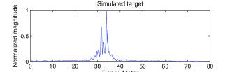
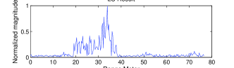
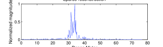
Figure 1: Comparison of result obtained via different methods for simulative data. (a) Model of scatters. (b) LS result of missing data. (c) Sparse recovery of missing data.

The results of simulation data obtained via different methods are compared in Fig.1. Fig.1(b) show the result obtained from LS method [4], Fig.1(c) demonstrate the result from new approach. From which it can be noted that LS method has created high sidelobe, and the result by new method is more similar to original target range profile.

Figure 2: Similarity measure.

To analyze the profiling results of the two methods quantitatively, we measure the similarity between the simulated target and the reconstruction profile by normalized cross correlation. Similarity equals $1$ means perfect reconstruction. Fig.2 illustrate the comparison. We increase the number of missing pulses from 0 to 20. The line marked by “$\vartriangle$” denotes the similarity by LS method, and line marked by “$\square$” denotes the similarity by sparse recovery. Sparse recovery has an obvious advantage over the LS counterpart.

IV-B Real Radar Data

We use real radar data obtained from SF radar. An experiment was carried out in a wide and flat field. A single metal reflector was placed 1010m away from the radar antenna. Experimental data of I/Q channels was collected from the baseband of the radar receiver. All parameters in the experiment were equal to the simulated data. We discard 12 pulses randomly to simulate the missing data condition. New approach is applied to the missing data. Profiling results are compared to IDFT based LS method.

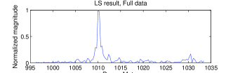
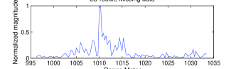
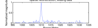
Figure 3: Comparison of result obtained via different methods for real radar data. (a) Full pulse recovery. (b) LS result of missing data. (c) Sparse recovery of missing data.

Fig. 3(a) shows the profiling result of LS method with full data. Fig. 3(b) and 3(c) compare the profiling results to the missing data by LS method and the new method respectively. LS method exhibits high sidelobe as predicted, while the profiling result by new method is similar to full data profiling. Sparse recovery outperforms LS using real radar data.

V Conclusion

The application of sparse recovery in extended HRR profiling for SF radar is illustrated. The simulated data and real data experiments prove that the proposed method is an appropriate tool to deal with missing data problem. Profiling quality of the new method has an obvious advantage over IDFT based least square method, if some pulses are missing. Moreover, it can profile multiple coarse-range-bins simultaneously, indicating a wide profiling range. The profiling result is not corrupted by ghost images. Further work should consider reducing computational load for real-time implementations.

References

- [1] EINSTEIN T.H., “Generation of high resolution radar range profiles and range profile autocorrelation functions using stepped frequency pulse trains,” Project Report TT-54, Massachusetts Institute of Technology, Lincoln Laboratory, 18 October 1984 (AD-A149242)
- [2] WEHNER D.R, High resolution radar, 2nd ed. Artech House, Norwood, MA, 1995.
- [3] L. Zhang, M. Xing, C. Qiu, J. Li, Z. Bao, “Achieving higher resolution ISAR imaging with limited pulses via compressed sampling,” IEEE Geoscience and Remote Sensing Letters, vol. 6, no. 3, pp. 567-571, July 2009.
- [4] Y. Liu, H. Meng, H. Zhang and X. Wang, “Eliminating ghost images in high-range resolution profiles for stepped-frequency train of linear frequency modulation pulses,” IET Radar Sonar Navig., 2009, Vol. 3, Iss. 5, pp. 512-520.
- [5] E. Cand s, J. Romberg, and T. Tao, “Robust uncertainty principles: Exact signal reconstruction from highly incomplete frequency information,” IEEE Trans. Inform. Theory, vol. 52, no. 2, pp. 489-509, Feb. 2006.
- [6] D. Donoho, “Compressed sensing,” IEEE Trans. Inform. Theory, vol. 52, no. 4, pp. 1289-1306, Apr. 2006.
- [7] R. Baraniuk, P. Steeghs, “Compressive radar imaging,” Proc. 2007 IEEE Radar Conf., Apr. 2007, pp. 128-133.
- [8] S. Shah, Y. Yu, A. Petropulu, “Step-frequency Radar with Compressive Sampling,” Available: http://arxiv.org/abs/0910.0886v1