Multiplicity and period distribution of Population II field stars in solar vicinity

Abstract

We examine a sample of 223 F, G and early K metal-poor subdwarfs $(\mathrm{[m/H]}<-1)$ with high proper motions ($\mu>0.2^{\prime\prime}/$ year) at the distances of up to $250$ pc from the Sun. By means of our own speckle interferometric observations conducted on the 6 m BTA telescope of the Special Astrophysical Observatory of the Russian Academy of Sciences, and the spectroscopic and visual data taken from the literature, we determine the frequency of binary and multiple systems in this sample. The ratio of single, binary, triple and quadruple systems among 221 primary components of the sample is 147:64:9:1. We show that the distribution of orbital periods of binary and multiple subdwarfs is asymmetric in the range of up to $P=10^{10}$ days, and has a maximum at $P=10^{2}-10^{3}$ days, what differs from the distribution, obtained for the thin disc G dwarfs (Duquennoy & Mayor, 1991). We estimated the number of undetected companions in our sample. Comparing the frequency of binary subdwarfs in the field and in the globular clusters, we show that the process of halo field star formation by the means of destruction of globular clusters is very unlikely in our Galaxy. We discuss the multiplicity of old metal-poor stars in nearby stellar streams.

1 Introduction

The study of metal-poor stars $(\mathrm{[Fe/H]}<-1)$ makes it possible to shed light on numerous problems of modern astrophysics, such as heavy elements production in supernova explosions, the metallicity distribution function of the stellar halo, the initial mass function, the nature of the Big Bang and the first generation, or Population III, stars, etc. An important place among these fundamental problems is occupied by the questions of the origin, chemical and dynamical evolution of our Galaxy. The oldest stars with the masses of $M\leqslant 0.8\ M_{\odot}$ are unevolved. Therefore, the abundance of chemical elements in their atmospheres reproduces the composition of prestellar matter. Additional information on spatial motions of these stars preserves the possibility to reconstruct the way the Milky Way formed.

The orbital elements of binary and multiple stellar systems are an important tool for studying prestellar matter. In single low mass stars, the mass is the only parameter conserved since the time of star formation. Binary and multiple systems bear three more conserved values: the angular momentum, the eccentricity and the mass ratio of their components (Larson, 2001) in case of detached systems. Therefore, binary and multiple stars carry more information on the process of star formation than single stars. The study of binary and multiple metal-poor systems enables us to impose certain restrictions on the physical conditions in prestellar matter at the time of the genesis of our Galaxy. Metal-poor stars are common in the globular clusters, galactic halo and in the galactic field, where an existence of the so-called stellar streams was revealed (e.g., Eggen 1996a, b). The multiplicity and the orbital parameters of binary and multiple stars in these streams may also provide additional information on the nature of the stream’s progenitor and its dynamical evolution.

The problem of stellar multiplicity was widely discussed in the literature, however, it mostly concerned the thin disc stars with solar-like metallicities (Duquennoy & Mayor, 1991; Fischer & Marcy, 1992; Halbwachs et al., 2003). Metal-poor stars were studied much less, as their occurrence in the solar neighbourhood is less than 1%, according to Nordstr$\mathrm{\ddot{o}}$m et al. (2004) catalog. Early works, addressing the rate of binary systems among Population II stars, showed that this value is small, as compared to the analogous value for Population I stars (Abt & Levi, 1969; Crampton & Hartwick, 1972; Abt & Willmarth, 1987). In subsequent works (Preston & Sneden, 2000; Goldberg et al., 2002; Latham et al., 2002) it was concluded that these values are indistinguishable (idem Abt 2008). A long-term spectroscopic monitoring of about $1\ 500$ nearby stars with high proper motions (Carney et al. 1994 (hereinafter CLLA), 2001; Goldberg et al. 2002; Latham et al. 2002) has played an important role in the study of the multiplicity of metal-poor stars. Spectroscopic studies cover the systems with relatively short orbital periods ($P\lesssim 10$ years).

The study of long-period couples with common proper motion components (Zapatero Osorio & Martin, 2004) confirms the hypothesis of an equal frequency of binary systems among the old and young stellar populations (idem Allen, Poveda & Herrera 2000). Meanwhile, an ‘intermediate’ period range of $P\approx 10-1\ 000$ years, which corresponds to the semi-major orbital axes of $a\approx 10-100$ AU in the solar neighbourhood, remains poorly understood to date. This range can be studied with the use of adaptive optics, speckle interferometry and long baseline interferometry. The scarce Population II stars observations, made by means of the interferometric techniques, were ran either for the brightest stars (Lu et al., 1987) or with relatively low angular resolution (Zinnecker, Kohler & Jahreiß, 2004). Notwithstanding the empirical data available to date, the number of known binary and multiple systems with metal-poor components remains small.

In order to enlarge the database of binary and multiple Population II stars, to define their orbital parameters and the properties of their components, we conducted speckle interferometric observations of 223 metal-poor subdwarfs with high proper motions located in the solar neighbourhood (Rastegaev, Balega & Malogolovets, 2007, 2008). The observations were made with the diffraction-limited resolution of the 6 m Big Telescope Alt-azimuthal (BTA) of the Special Astrophysical Observatory of the Russian Academy of Sciences ($0.023^{\prime\prime}$ at the wavelength of 550 nm). In the present work, we analyse the multiplicity and orbital periods distribution for binary and multiple stars. We made our analysis based on own observations and the data adopted from other authors. Additionally, an attempt was made to examine the ratio of binary and multiple stars in the streams of old metal-poor stars located in the solar neighbourhood.

2 Sample

For the observations with high angular resolution, we compiled a sample of 223 field subdwarfs of the F, G and early K spectral classes (Rastegaev et al., 2007) from the CLLA catalog. The CLLA presents a spectroscopically studied sample of the A–K spectral types dwarfs from the Lowell Proper Motion Survey (Giclas, Burnham & Thomas, 1971, 1978), which mainly includes the stars from the Northern Hemisphere with proper motions exceeding $0.26^{\prime\prime}$ per annum and brighter than $16^{m}$ in the $B$ band.

We selected 223 stars from the CLLA using the following criteria:

• metallicity $\mathrm{[m/H]}<-1$,

• declination $\delta>-10^{\circ}$,

• apparent magnitude $\mathrm{m_{V}}<12^{m}$.

The last criterion was determined by the limiting stellar magnitude of our speckle interferometer (Maximov et al., 2003), which was about $13^{m}$. No restrictions were applied on the heliocentric distances of these stars, evenly distributed on the celestial sphere. The maximum distance to the sample objects is 250 pc. The median heliocentric distance of the selected stars is approximately $100$ pc. This allows us to take advantage of high angular resolution in order to detect new systems, since at such distances the pairs with semi-major orbital axes from 10 to 100 AU are hard to detect both spectroscopically and visually.

Using the two following criteria, $\mu>0.26\ ^{\prime\prime}/$year and $\mathrm{[m/H]}<-1$, we tried to rule out the thick and thin disc stars. In case of the thick disc though, these limits are not stringent and some objects may belong to the metal-weak tail of the thick disc (Arifyanto et al., 2005).

To separate the halo stars from the disc stars in our sample, we used a formal method, described in the appendix of Grether & Lineweaver (2007). The equations establishing the probability that a star belongs to the thin disc ($P_{\rm thin}$), the thick disc ($P_{\rm thick}$) or the halo ($P_{\rm halo}$) are

$$P_{\rm thin}=f_{1}\frac{P_{1}}{P}\;,\;P_{\rm thick}=f_{2}\frac{P_{2}}{P}\;,\;P_{\rm halo}=f_{3}\frac{P_{3}}{P},$$ (1)

where

$$P=\sum f_{i}P_{i},$$

$$P_{i}=C_{i}\exp\left[-\frac{U^{2}}{2\sigma_{U_{i}}^{2}}-\frac{(V-\langle V\rangle)^{2}}{2\sigma_{V_{i}}^{2}}-\frac{W^{2}}{2\sigma_{W_{i}}^{2}}-\right.$$

$$\left.-\frac{([\mathrm{Fe/H}]-\langle[\mathrm{Fe/H}]_{i}\rangle)^{2}}{2\sigma_{[\mathrm{Fe/H}]_{i}}^{2}}\right],$$

$$C_{i}=\frac{1}{\sigma_{U_{i}}\sigma_{V_{i}}\sigma_{W_{i}}\sigma_{[\mathrm{Fe/H}]_{i}}},$$

$$i=\mathrm{1\ (thin\ disc),\ 2\ (thick\ disc),\ 3\ (halo).}$$

The input parameters for these equations are adopted from Robin et al. (2003), and presented in Table 1. We rejected three out of 221 systems: two double stars G99-48 and G166-45, and one single BD $-1^{\circ}1792$, because for these systems there are no heliocentric distances or $UVW$ components in the CLLA. We referred the objects with $P_{\rm halo}>0.5$ to the halo stars. There is a total of 148 of such stars in our sample. The remaining 70 objects belong to the thick disc. None of the stars from the sample have $P_{\rm thin}$ exceeding $0.01$. Average metallicity and space velocity vector components for halo stars in our sample are: $(\langle[\mathrm{Fe/H}]_{halo}\rangle,\langle U_{halo}\rangle,\langle V_{halo}\rangle,\langle W_{halo}\rangle)=$ ($-1.9\pm 0.5$, $-16\pm 152$ km/s, $-180\pm 81$ km/s, $-1\pm 78$ km/s), where the errors are standard deviations. In a similar way, these values for the thick disc stars are: $(\langle[\mathrm{Fe/H}]_{thick}\rangle,\langle U_{thick}\rangle,\langle V_{thick}\rangle,\langle W_{thick}\rangle)=$ ($-1.2\pm 0.2$, $-12\pm 83$ km/s, $-92\pm 59$ km/s, $3\pm 50$ km/s). However, the system of equations (1) might be unable to accurately describe the situation in the areas where the star parameters of different Populations overlap.

Fig. 1 shows the distribution of the sample stars on the graph metallicity versus $V$-component of spatial velocity, data taken from the CLLA. The halo stars with a substantial dispersion of spatial velocities and with low metallicities are located in the central and left parts of the figure. At the top right of the figure, along with the halo stars, there are stars of the thick disc’s metal-weak tail (Arifyanto et al., 2005).

The sample consists of main sequence stars and seven blue stragglers (Carney et al., 2001, 2005b), — a continuation of the main sequence in the area of hotter and bluer stars, as compared to the turnoff stars. Fig. 2 represents the location of the sample stars in the Hertzsprung-Russell diagram compared to the old population of the M13 globular cluster with $\mathrm{[Fe/H]}=-1.61$ (Grundahl, VandenBerg & Andersen, 1998).

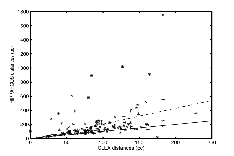
Figure 3: A comparison between the trigonometric distances from the HIPPARCOS catalog (van Leeuwen, 2007) and photometric distances from the CLLA for 133 sample stars. The dotted line is a linear regression $y=-18.58+2.23x$. $r=0.42$ is the correlation coefficient. The solid line represents the $y=x$ function.

Fig. 3 represents a comparison between the trigonometric and photometric distances for the sample stars. The parallaxes for 135 sample stars were taken from the HIPPARCOS satellite data (van Leeuwen, 2007). The corresponding photometric distances for 133 stars are retrieved from the CLLA. We can see that the distances, obtained with HIPPARCOS, are systematically larger than the corresponding distances from the CLLA. This difference can be explained by some unaccounted components, the presence of which may lead to an underestimation of photometric distances. Another reason for this discrepancy is the photometric distance calibration adopted in the CLLA.

Most of the stars in our sample were examined for common proper motion components (Allen et al., 2000; Zapatero Osorio & Martin, 2004).

3 Observations and results

The speckle interferometric observations of 223 sample stars were carried out in 2006–2007 on the 6 m BTA telescope (Rastegaev et al., 2007, 2008) which diffraction-limited resolution is $0.023^{\prime\prime}$ for $\lambda=550$ nm and $0.033^{\prime\prime}$ for $\lambda=800$ nm. Most of the observations were carried out using the system (Maksimov et al., 2009) based on a 512$\times$512 EMCCD (a CCD featuring on-chip multiplication gain) with high quantum efficiency and linearity. This system allowed us to detect objects with magnitude differences between the components of up to $\triangle m=5^{m}$. Taking into account the limiting stellar magnitude of our sample ($\mathrm{m_{V}}<12^{m}$), detected secondary component can be as faint as $17^{m}$. The $4.4^{\prime\prime}$ field of view of our system allows detection of secondary components at a separation of $3^{\prime\prime}$ from the primary star. The speckle interferograms were recorded using five filters: $545/30$, $550/20$, $600/40$, $800/100$ and $800/110$ nm (the first number indicates the central wavelength of the filter, the second — the half-width of the filter’s bandwidth) with the exposures of 5 to 20 ms. For each object, we accumulated from 500 to $2\ 000$ short exposure images depending on weather conditions. The observations were made with an average seeing of $1.5^{\prime\prime}$. The accuracy of our speckle interferogram processing method (Balega et al., 2002) may be as good as $0.02^{m}$, $0.001^{\prime\prime}$, and $0.1^{\circ}$ for the component magnitude difference, angular separation and position angle respectively.

For 19 stars in our sample we observed the speckle interferometric companions. Sixteen companions were resolved astrometrically for the first time. We discovered 5 new binary systems (G191-55 (catalog ), G114-25 (catalog ), G142-44 (catalog ), G28-43 (catalog ), G130-7 (catalog )), 3 triple systems (G87-47 (catalog ), G111-38 (catalog ), G190-10 (catalog )) and one quadruple system, G89-14 (catalog ). The position parameters and magnitude differences between the speckle interferometric components are listed in tables 1 and 2 of Rastegaev et al. (2008).

4 Sample completeness

To be able to determine the completeness of our sample, we used the star count method. From all known subdwarfs within 25 pc from the Sun, we selected 5 objects with absolute magnitudes $M_{V}<8^{m}$ and metallicities $\mathrm{[Fe/H]}<-1$ (see tab. 1 in Fuchs & Jahreiß 1998). The star GJ 1064 A, with the metallicity of $-1$ dex, was as well included in our sample. An extrapolation to the volume of our sample (with the radius of $\approx 250$ pc) increases the number of such objects to $\approx 5\ 000$. Obviously, when we consider the frequency of stars in different volumes, we cannot depart from the uniform distribution of stars in space. We have to bear in mind the structure of the Galaxy and the data available on the star distribution in its various subsystems. However, as we show in the Appendix, for the stars in our sample located within 250 pc from the Sun, the structure of our Galaxy can be neglected. Therefore, the number of objects in our sample constitutes about $5\%$ from the total number of stars in question located in the examined region of space. We have to mention that while examining the stars in different volumes, we were taking account of the primary components only in case of spectroscopic and speckle interferometric pairs, and of both components in the case of visual and common proper motion pairs.

5 Undetected companions

Capability to detect a binary system is determined by both the observations method used and by the physical characteristics of the system itself. As the sample objects were examined using three different methods, — spectroscopic, speckle interferometric and visual, we have to analyse the number of systems unaccounted for by each of these methods. To do that, we conditionally divided the spectroscopic and astrometric pairs by the values of their semi-major axis at $a<10$ AU and $a>$ 10 AU, and their orbital periods at $P<10\ 000$ days and $P>10\ 000$ days, respectively.

For spectroscopic pairs, we hypothesized that the component mass ratio is uniformly distributed from 0 to 1, then took the deduced period distribution for the studied stars in the range of 0 to $10\ 000$ days (see below), and made our calculations using the formulae from Mazeh, Latham & Stefanik (1996). Our conclusion is that the probability of not detecting a binary system approximately equals to $20\%$.

As for the visual and interferometric binaries, the secondary can be detected if the following two conditions are satisfied. Firstly, the magnitude difference between the components should not exceed a certain critical value, determined by the detector’s dynamical range and the spectral range used. Secondly, in case of speckle interferometry, the angular separation between the components should be larger than the telescope’s diffraction limit and smaller than the detector’s field of view, or, in case of visual studies, the angular separation should be smaller than the certain restrictions imposed.

In order to estimate the number of unresolved systems due to the effect of ellipse projection of the true orbit on the picture plane, and due to the secondary component’s orbital phase at the moment of observation, we used the Monte Carlo simulation. We modelled a sample of stellar orbits, evenly distributed in space, with heliocentric distances from 25 to 250 pc, uniformly distributed eccentricities (from 0 to 0.9) and arguments of periapsis (from 0 to 360 ^∘). Inclinations of the true orbits to the picture plane obey the sin $i$ law.

The resulting orbits were projected onto the picture plane using the following formulae (Couteau, 1981)

$$\rho=\frac{a\ (1-e^{2})}{1+e\ \mathrm{cos}\ \upsilon}\ \frac{\mathrm{cos}\ (\upsilon+\omega)}{\mathrm{cos}\ (\theta-\Omega)},$$

$$\mathrm{tg}\ (\theta-\Omega)=\mathrm{tg}\ (\upsilon+\omega)\ \mathrm{cos}\ i,$$ (2)

$$\mathrm{tg}\ \frac{\upsilon}{2}=\sqrt{\frac{1+e}{1-e}}\ \mathrm{tg}\ \frac{u}{2},$$

$$M=u-e\ \mathrm{sin}\ u,$$

where $\rho$ is the angular separation between the components in the picture plane, $a$ is the orbital semi-major axis (in arcseconds), $e$ is eccentricity, $\upsilon$ is the true anomaly, $u$ is the eccentric anomaly, $M$ is the mean anomaly, $\omega$ is the argument of periapsis, $\theta$ is the position angle of a secondary component, $\Omega$ is the longitude of an ascending node and $i$ is the inclination angle between orbital and picture planes.

Further, a random orbital position of the satellite was predetermined for each simulated system. At this point we accounted for the fact that a companion spends more time at apoastron than at periastron. Then the projection distances $\rho$ from the satellite to the primary star were counted. A relative number of projection distances greater than $0.033^{\prime\prime}$(the diffraction limit of the 6 m telescope in a 800/100 filter) is, in fact, the probability value of a system detection using the speckle interferometric and visual methods. The results of modelling show that for the systems with an orbital semi-major axis exceeding $a=10$ AU, such probability is close to 1 and an influence of the components’ geometry can be neglected. This probability weakly depends on the choice of a plausible distribution of semi-major axis for $a>10$ AU.

Let’s consider now the incompleteness of detection caused by the magnitude difference between the components. An average mass of a primary star in our sample is $0.65\ M_{\odot}$ and a standard deviation is $\sigma_{{\textrm{\tiny M}}}\approx 0.05\ M_{\odot}$. The maximum magnitude difference between the components, detected by speckle interferometric and visual methods, is about $5^{m}$ (Maksimov et al., 2009; Zapatero Osorio & Martin, 2004). For speckle interferometry, we used a more conservative estimate of $4^{m}$. According to the model of Baraffe et al. (1997) for $\mathrm{[Fe/H]}=-1$, the minimal mass of a secondary, which is 4 mag fainter than a primary of an average mass, equals $M_{min}=0.20\ M_{\odot}$ in the $I$ band. This band roughly corresponds to our 800/100 and 800/110 filters. To compute the number of undetected companions, we have to know the function of mass ratio distribution. We used a uniform distribution. If the mass ratio for wide (speckle interferometric, visual and CPM) pairs obeys a uniform $q$ distribution, then from the following ratio

$$\frac{\int\limits^{M_{2}=M_{min}}_{M_{2}=0.08}\ dM_{2}}{\int\limits^{M_{2}=0.8}_{M_{2}=M_{min}}\ dM_{2}},$$ (3)

we find the quantity of secondary components with masses in the range from $0.08\ M_{\odot}$ (mass of a brown dwarf) to $M_{min}$ per one secondary component with the mass in the range from $M_{min}$ to $0.8\ M_{\odot}$ (a maximal mass of the stars in our sample). This quantity equals 0.2. Therefore, a fifth of discovered speckle interferometric companions remains undetected at the given distribution of $f(q)$ with the use of 800/100 (or 800/110) filter. For the 550/20 and 545/30 filters, $M_{min}=0.28\ M_{\odot}$ and the expression (3) is approximately 0.38, which makes these filters less suitable for our task in the sense of magnitude difference (yet, more suitable from the viewpoint of the angular resolution). The search for common proper motion pairs for the sample stars was conducted in the $I$ band (Zapatero Osorio & Martin, 2004). Forty seven objects from our sample were observed speckle interferometrically, solely using the 550/20 or 545/30 filters, 9 objects were observed only in the 600/40 filter and one object (G183-9) was observed in the 550/20 and 600/40 filters. The 166 remaining stars were at least once observed in the 800/100 or 800/110 filters. With this in mind, we find that the expression (3) is approximately equal to 0.25 for all filters. Therefore, according to these rough estimates, for 33 astrometric components in our sample (see Fig. 4) we have about 8 unaccounted companions or 24%; that is comparable to 20% of unaccounted spectral companions. Thus, we can assume that the number of unaccounted components in our sample does not depend on the orbital period and is $20-25\%$.

Analogously, the IMF-like distribution $f(q)\sim q^{-1.3}$ for $0.08\leq M/M_{\odot}<0.5$ (Kroupa, 2001) gives us 37 unaccounted companions. In case $f(q)$ grows towards bigger $q$ values (Soderhjelm, 2007), then the number of undetected astrometric components in our sample does not exceed 5. For our further estimates we chose the values corresponding to the uniform $q$ distribution.

6 Multiplicity of the sample

6.1 Raw estimates

In order to calculate the ratio of the systems of different multiplicity among the studied stars, we complemented the results of our speckle interferometric measurements by the data from spectroscopic and visual studies found in literature. The information on the spectroscopic companions was adopted from the publications dedicated to long-term spectroscopic monitoring of Population II stars by Carney, Latham, Laird et al. (CLLA; Carney et al. 2001; Goldberg et al. 2002; Latham et al. 2002; Latham 2008). The data on wide visual pairs was taken from Allen et al. (2000) and Zapatero Osorio & Martin (2004) via the WDS catalog (Mason et al., 2001). As a result, the ratio of single:binary:triple:quadruple ($S:B:T:Q$) systems for the stars in our sample is 147:64:9:1 (Rastegaev et al., 2007, 2008). Therefore, at least 159 stars from 306 stars in our sample (221 main components and 85 satellites) belong to binary and multiple systems. The multiplicity of our sample is $33\%^{+7\%}_{-6\%}$, where multiplicity is understood as the ratio of binary and multiple systems to the total number of systems

$$f_{systems}=\frac{B+T+Q}{S+B+T+Q}.$$

A similar, unadjusted for unresolved companions value for the thin disc stars of spectral classes from F7 to G9, equals to 51:40:7:2 (Duquennoy & Mayor, 1991), with the multiplicity of about 50%. It is necessary to pay attention to the differences between the two compared samples. When our sample was formed from the stars with a certain apparent magnitude limit and high proper motions, the sample from Duquennoy and Mayor is only limited by the heliocentric distances (all their stars are located within 22 pc from the Sun).

In terms of multiplicity, the Population II stars differ from the Population I. At least a third of metal-poor systems and at least half of the systems with solar like abundances are binary and multiple. This discrepancy can be explained by both the complexity of detection of low mass metal-poor spectroscopic satellites, by the selection effects, and by the dynamical evolution of binary and multiple stars.

6.2 Corrected estimates

To estimate the true multiplicity of the sample stars, we have to account for various selection effects that are unavoidable in astronomical observations. The five underlaying criteria for the choice of stars in our sample are: proper motion ($\mu>0.26\ ^{\prime\prime}/$year), metallicity ($\mathrm{[m/H]}<-1$), magnitude ($\mathrm{m_{V}}<12^{m}$), spectral classes (F, G and early K), and position in the sky (all our stars are located in the Northern hemisphere). We also have to take into account the undetected companions (Section 5).

For the sake of simplicity we assume that the multiplicity of a stellar Population does not depend on proper motion and position in the sky. This gives us grounds to disregard the selection effects related to the proper motion of the stars and their coordinates.

To account for the bias incurred by magnitude, we have to consider the $\mathrm{\ddot{O}}$pik effect ($\mathrm{\ddot{O}}$pik, 1923; Goldberg, Mazeh & Latham, 2003), which applies to binaries detected within a magnitude-limited sample of stars. This effect is an expansion of the Malmquist effect for binary stars. Binaries are on the average brighter than singles. Thus, in a magnitude-limited sample the binaries are observed from a bigger volume in space than the single stars. To avoid this effect we rejected the binaries which are brighter than $12^{m}$ due to the contribution of the secondary component to the total luminosity. For SB1 binaries we adopted that the luminosity of the secondary component is not less than 2 magnitudes fainter than the primary (Goldberg et al., 2002). We discarded the SB1 pairs whose primary component was fainter than $12^{m}$ in the assumption that the secondary component is 2 magnitudes fainter than the primary. For SB2 pairs the luminosity of the primary component was determined from the total luminosity of the system and the mass ratio of the components (Goldberg et al., 2002) using evolutionary tracks from Baraffe et al. (1997). We thus rejected four binaries, one SB1 (G242-14) and 3 SB2 (G86-40, G99-48, G183-9) as the measured luminosities of the primaries are fainter than 12 magnitude in the $V$-band. In the worst case for SB2 systems we have to discard 4 pairs in the assumption that for a given integrated magnitude the luminosities of primary and secondary components are equal. None of the speckle interferometric pairs have been excluded from consideration due to the $\mathrm{\ddot{O}}$pik effect. The magnitude differences between the components measured by us for a given integrated magnitude suggest that the primary components of the speckle pairs are brighter than $12^{m}$. Not a single system of higher multiplicity was dropped from the analysis as their primaries are not compliant with the condition $m_{V}>12^{m}$.

Taking into account an adjustment for unresolved components and $\mathrm{\ddot{O}}$pik effect, the multiplicity of F, G and early K subdwarfs in the solar neighbourhood is, according to our calculations, at least $40\%$ and at least $60\%$ for the thin disc G dwarfs (Duquennoy & Mayor, 1991). In both cases correction does not exceed $10\%$.

6.3 Multiplicity as a function of metallicity

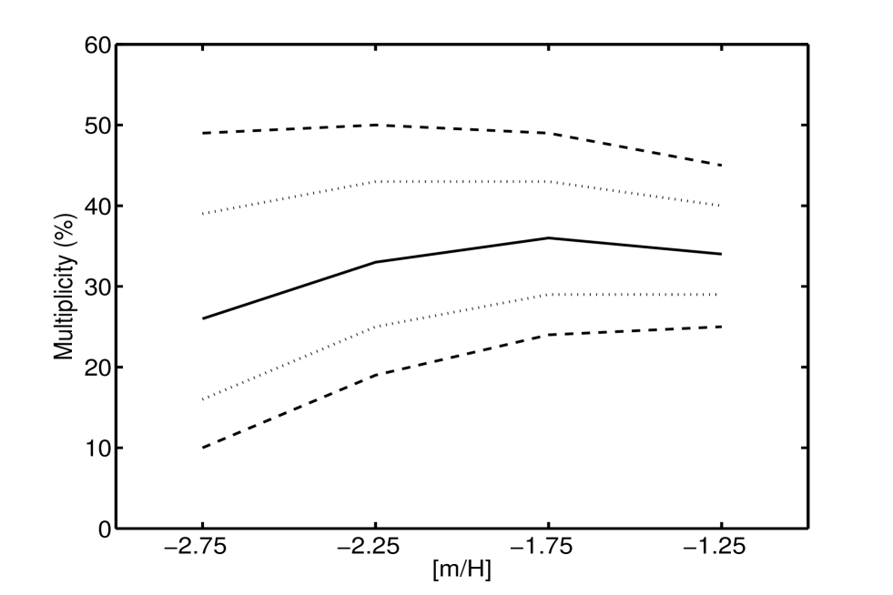
Figure 5: Multiplicity versus metallicity for stars in our sample (solid line). Dashed lines mark the 95 % confidence interval. Dotted lines mark the 70 % confidence interval.

To investigate the effect of metallicity on the multiplicity of stars in our sample, we divided it into four metallicity bins: $(-3,-2.5]$, $(-2.5,-2.0]$, $(-2.0,-1.5]$, $(-1.5,-1.0)$. One single star, G64-12 with $\mathrm{[m/H]}=-3.52$ was rejected from the analysis. In every bin we evaluated the ratio of single:binary:triple:quadruple systems and multiplicity $f_{systems}$. The acquired results are presented in Table 2, whereof it is clear that in the range $\mathrm{[m/H]}$ from $-2.5$ to $-1.0$ the multiplicity does not depend on metallicity and constitutes one third. In the range $(-3,-2.5]$ the multiplicity is somewhat lower, but the number of systems in this range is smaller than in the rest of ranges, which affects the accuracy of determination of $f_{systems}$ (see Fig. 5). It can be seen from Fig. 5 that in the first approximation the rate of binary and multiple systems in our sample feebly depends on metallicity. Carney et al. (2005a) obtained analogous results based on a bigger sample of stars, studied spectroscopically. Note that the bulk of our triple stars belong to the range $\mathrm{[m/H]}=(-1.5,-1.0)$.

6.4 Halo versus thick disc

Using the set of equations (1) we separated the stars of the thick disc and the halo stars in our sample. The ratio single:binary:triple:quadruple systems for thick disc stars is 46:19:5:0, and the multiplicity $f_{systems}=34\%^{+13\%}_{-11\%}$. The same for the halo stars $S:B:T:Q=$101:45:4:1, and $f_{systems}=33\%^{+8\%}_{-7\%}$.

An independence of the ratio of binary and multiple systems from the conditional division ’thick disc-halo’, as well as the consistency of $f_{systems}\approx 33\%$ under metallicity changes (Table 2) might testify that most of the stars in our sample belong to one and the same galactic subsystem, the halo. Note again that the set of equations (1) might not be operable in cases when the stellar parameter ranges of different galactic subsystems overlap. It is not impossible though that the Population II stars, both the halo and thick disc stars have similar ratios of the systems of different multiplicity.

6.5 Multiplicity as a function of kinematics

Table 3 represents the basic facts on the dependence of multiplicity of the sample stars on kinematics. We excluded three objects from consideration: two double stars G99-48 and G166-45, and one single BD $-1^{\circ}1792$, because for them there are no distances or $UVW$ components in the CLLA. For single and binary and mltiple stars the average values and standard deviations of the space velocity vector components are: $\langle U_{s}\rangle=-13\pm 137$ km/s, $\langle U_{b+m}\rangle=-18\pm 127$ km/s, $\langle V_{s}\rangle=-160\pm 86$ km/s, $\langle V_{b+m}\rangle=-135\pm 81$ km/s, $\langle W_{s}\rangle=2\pm 74$ km/s, $\langle W_{b+m}\rangle=-3\pm 61$ km/s. For norm of velocity vector $v=\sqrt{U^{2}+V^{2}+W^{2}}$: $\langle v_{s}\rangle=222\pm 89$ km/s, $\langle v_{b+m}\rangle=196\pm 80$ km/s. In the first approximation we may consider that for our stars the multiplicity is constant and does not depend on the spatial velocity vector components.

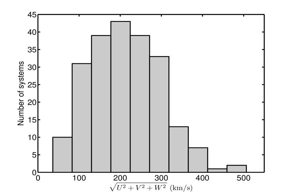
Figure 6: Norm of velocity vector distribution for stars in our sample.

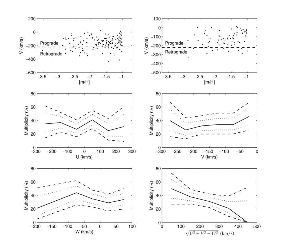
Figure 7: The upper panel shows $V$ versus $\mathrm{[m/H]}$ dependence for single (left part) and double and multiple (right part) stars. Middle and lower panels show the frequency of double and multiple stars depending on the components of the velocity vector and its norm. Dashed lines mark the 95% confidence interval. Dotted lines mark the 70% confidence interval.

The distribution of the norm of spatial velocity vector $v=\sqrt{U^{2}+V^{2}+W^{2}}$ for stars in our sample is shown on Fig. 6. The average value of this norm is 214 km/s with the standard deviation 86 km/s. Fig. 7 shows the $V$ versus $\mathrm{[m/H]}$ dependence for single (left upper panel) and double and multiple (right upper panel) stars in our sample. Middle and lower panels of this figure show the dependence of the multiplicity of our stars on four kinematic parameters $UVW$ and $v$. The figure shows that the frequency of double and multiple stars in our sample weakly depends on the change of $UVW$ components. We can draw lines corresponding to a constant multiplicity of approximately 35% within a 70% confidence level (see middle panel and left lower panel). For norm of spatial velocity vector a trend of decreasing multiplicity with increasing $v$ is seen (see right lower panel). The data in the 95% confidence level do not contradict the hypothesis $f_{systems}(v)=const$ or a small growth of multiplicity with the increase of $v$. Nevertheless, with the probability of at least 70% we can say that with the increase of the norm of spatial velocity vector the frequency of double and multiple systems in our sample falls. Most likely, the bigger the spatial velocity of a star, the less the probability that it has a companion.

Forty five from 223 stars in our sample are moving on retrograde galactic orbits ($V<-220$ km/s), i.e. in the opposite direction to the rotation of our Galaxy. For these stars, the ratio of single:binary:triple:quadruple systems is 32:12:1:0 and their multiplicity is $29\%^{+15\%}_{-13\%}$. Carney et al. (2005a), analyzing a sample of 374 stars on highly retrograde orbits ($V<-300$ km/s) showed, that the frequency of spectroscopic binaries among them is two times smaller than that for the stars moving along with the Galaxy’s rotation. Our data, bearing an analysis of a wide range of periods, do not contradict their findings, yet, an insignificant number of highly retrograde objects in our sample does not allow us to make any definitive conclusions.

7 Period distribution

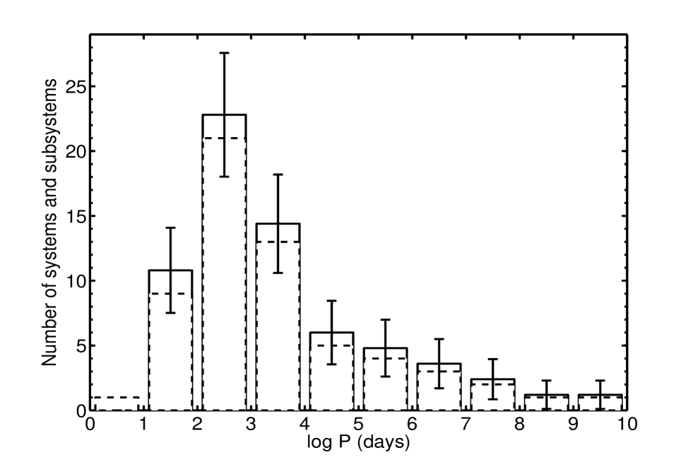
Figure 8: Period distribution for 60 binary stars in our sample (dashed line). The solid line marks the same distribution but corrected for $\mathrm{\ddot{O}}$pik effect and unresolved components. Error bars represent square roots from the number of stars in each bin.

The distribution of orbital periods for binary stars in our sample is shown in Fig. 8. The periods of spectroscopic pairs are taken from Goldberg et al. (2002) and Latham et al. (2002). The periods of astrometric pairs were derived with the help of the generalized Kepler’s third law on the basis of an empirical relation of the projected angular separation between the components and the semi-major axis. Knowing the system’s parallax $\pi$ and the projected angular separation between the components $\rho$, the expected value of the semi-major axis is calculated using the formula from Allen et al. (2000)

$$\left\langle a\right\rangle=\mathrm{antilog}\left[\mathrm{log}\frac{\rho}{\pi}+0.146\right],$$ (4)

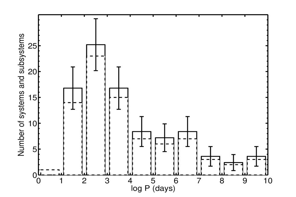
Figure 9: Period distribution for 60 binary stars and 21 subsystems of 10 multiple stars in our sample (dashed line). The solid line marks the same distribution but corrected for $\mathrm{\ddot{O}}$pik effect and unresolved components. Error bars represent square roots from the number of stars in each bin.

where $\left\langle a\right\rangle$ is expressed in astronomical units, $\rho$ and $\pi$ in arcseconds. Taking each system individually, we derived the sum mass of the components from the temperatures of the primary (CLLA) and secondary components, and from the magnitude difference, if the temperature of the secondary was unknown. To do this, we used models from Baraffe et al. (1997). Angular distances $\rho$ between the components of astrometric pairs were obtained from speckle interferometric observations or adopted from Allen et al. (2000) and Zapatero Osorio & Martin (2004). If the systems parallaxes were known from the HIPPARCOS catalog with an accuracy of better than $30\%$, we used them instead of the distances cited in the CLLA catalog. As a result, we were able to determine the periods for 60 binary systems out of 64 in our sample. The periods for the four remaining suspected binary systems, — G186-26 (catalog ) and G210-33 (catalog ) and two blue stragglers, BD +25^∘ 1981 (catalog ) and G43-3 (catalog ) (Carney et al., 2001), are too long to be determined (Latham, 2008). The period distribution for 60 binaries and 10 multiple systems (18 subsystems of 9 triple stars and 3 subsystems of a quadruple star G89-14), is shown in Fig.  9. The distributions corrected for $\mathrm{\ddot{O}}$pik effect and unresolved components on Fig. 8 and 9 are marked by a solid line.

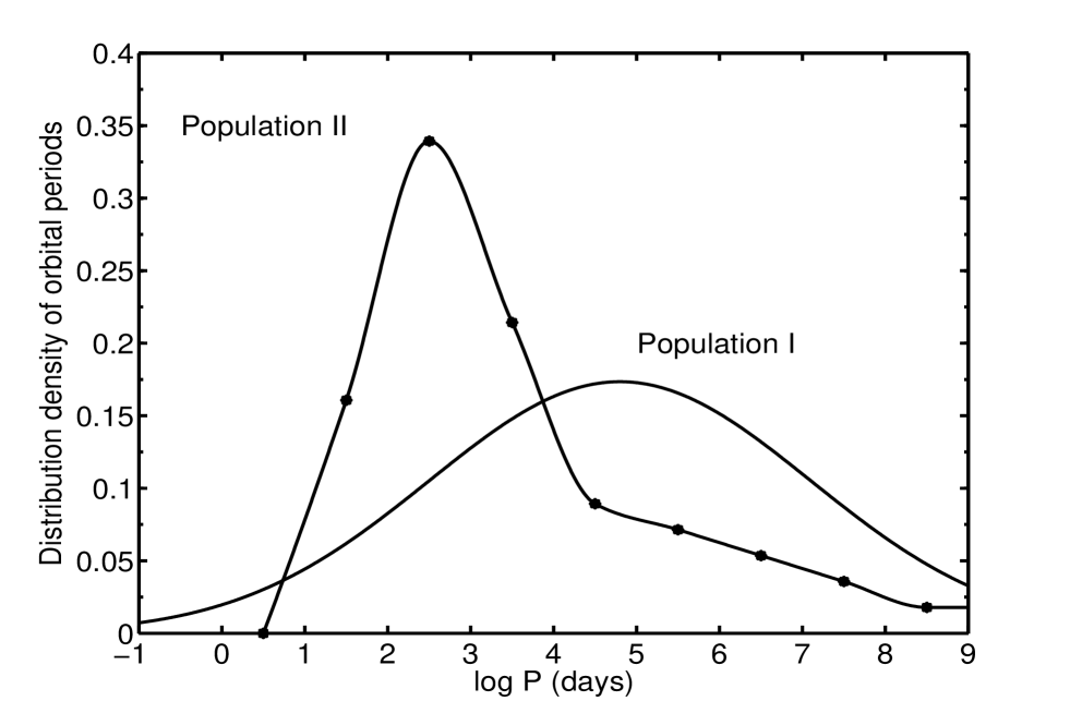
Figure 10: Distribution of densities of orbital periods for binary stars in our sample (Population II) interpolated by a cubic spline and idem for the thin disc stars (Population I), approximated by a Gaussian in Duquennoy & Mayor (1991).

Let’s compare the resulted distribution with an analogous one for the thin disc stars (Fig. 10). The maximum of an unsymmetrical period distribution for the stars in our sample lays in the range of $\log P=2-3$ dex (i.e. hundreds of days). For Population I stars, the $\log P$ distribution, which Duquennoy and Mayor approximated by a Gaussian, has a maximum in the range of $4-5$ dex (tens of thousands of days). An important feature of our distribution is a small number of short period ($\log P<1$) pairs. This range is represented by the only SB2 star G183-9 (catalog ) with a period of about 6 days (Goldberg et al., 2002), which is excluded while accounting for the $\mathrm{\ddot{O}}$pik effect.

To make a homogeneity check of the two samples, we conducted a nonparametric $\chi^{2}$ test (Kremer, 2007). By an accidental coincidence, the number of compared periods equals to 81 for each population. The test shows that the hypothesis of uniformity (i.e. common general population of two samples) can be rejected with a more than 95% probability.

Both distributions (Fig. 10) may be distorted by the selection effects. However, the differences in both the shape of the distributions and the location of the maxima could be induced by the dynamical evolution, undergone by the Population II stars. For example, a small quantity of old systems with periods of more than ten thousand days may be the result of a dynamical evolution at the stage of Galaxy formation. According to a recent concept, a bigger part of the stellar halo in our Galaxy was formed from small galactic systems (Bell et al., 2008). It is quite likely that at the stage of accretion of small galaxies-satellites of the Milky Way and their destruction, the physical conditions were favourable for dissociations of wide pairs with low binding energy. Attempting to explain the period distribution of Population II stars by a destructive impact of giant molecular clouds and other local perturbations of the gravitational potential of our Galaxy on the old stars orbiting around the galactic centre (Weinberg, Shapiro & Wasserman, 1987), is quite problematic. Such objects spend most of their lifespans away from the galactic plane.

8 Interesting triple and quadruple systems in our sample

In this section we will examine two old multiple systems that we find remarkable: a triple system G40-14 (catalog ) and a quadruple G89-14 (catalog ). Such objects are of great interest for the studies of the dynamical evolution and for the checks of various criteria of dynamical stability. In Table 4, we listed all the detected systems from our sample having more than 2 components. From ten multiple systems, nine are triples and only one is quadruple.

The uniqueness of the triple system G40-14 is in its retrograde galactic orbit with $V\approx-230$ km/s (CLLA). The inner subsystem of G40-14 is an SB1 pair with a period of $60.615$ days (Latham et al., 2002). The outer subsystem is formed by a visual component, which is located $98^{\prime\prime}$ away from the spectroscopic pair. Assuming that the system’s heliocentric distance is 235 pc, the expected semi-major axis is $\left\langle a\right\rangle\approx 30\ 000$ AU (Allen et al., 2000). We made a check for retrograde objects in the latest version (dated 13 August 2007) of the Multiple Star Catalog (Tokovinin, 1997), which is a compilation of 1158 known stellar systems with three or more components. In order to do that, we calculated the $U$ $V$ $W$ components of spatial velocities for the catalog stars from the cited parallaxes, radial velocities and proper motions, using the formulae from Johnson & Soderblom (1987). It appeared that only one object, a triple system ADS 16644 (catalog ), is moving on a retrograde galactic orbit ($V\approx-330$ km/s). Hence, G40-14 is the second of all known systems with more than two components moving against the rotation of the Galaxy.

G89-14 (for details, see Rastegaev 2009) is a system with the highest multiplicity in our sample. It consists of four components (Fig. 11): an SB1 pair AB with a period of 190 days (Latham et al., 2002), a speckle interferometric component C located at $\approx 1^{\prime\prime}$ from this SB1 pair (Rastegaev et al., 2007) and a common proper motion companion D at $34^{\prime\prime}$ (Allen et al., 2000). Based on the data from Allen et al. (2000), the evolutionary tracks from Baraffe et al. (1997), and on our speckle interferometric measurements, we evaluated the period ratio of the three G89-14 subsystems: 0.52 : 3 000 : 650 000 yr. Another well-known metal-poor quadruple system is NQ Ser (catalog ) (Tokovinin, 1997) with $\mathrm{[Fe/H]}=-1.05$ (Nordstr$\mathrm{\ddot{o}}$m et al., 2004). This multiple star was repeatedly observed on the BTA by means of speckle interferometry (e.g., Balega et al. 2006). According to our information, G89-14 with $\mathrm{[m/H]}=-1.9$ (CLLA) is the most metal-poor quadruple system known to date, which makes it an interesting object for a more detailed study.

9 Multiplicity of metal-poor stellar streams

Stellar streams (e.g., Eggen 1996a, b) are associations of stars possessing similar kinematics and metallicity. The study of such streams allows restoring to a certain degree the picture of the formation of various dynamical structures in our Galaxy. Traditionally, the stellar streams are being selected in a certain phase space and then their origin is interpreted using the data of spectroscopic analysis. In a phase space, a fine structure like stellar multiplicity can give additional information on the dynamical evolution of the stream and its primogenitor. However, until now it was not taken into due consideration.

The following six stars of our sample: G10-4 (catalog ), G13-9 (catalog ), G60-48 (catalog ), G24-3 (catalog ), G18-54 (catalog ), G28-43 (catalog ), are part of the Kapteyn’s star (catalog ) moving group (Eggen, 1996a), 10 other objects: G130-65 (catalog ), G75-56 (catalog ), G5-35 (catalog ), G40-14 (catalog ), G114-25 (catalog ), G11-44 (catalog ), G13-35 (catalog ), G183-11 (catalog ), G182-32 (catalog ), G126-52 (catalog ), belong to the Ross 451 (catalog ) moving group (Eggen, 1996b). In Table 5 we are listing some characteristics of these two halo streams. In the penultimate column of the table, you can see the ratio of single, binary and triple systems for the group members in our sample. In the last column, an analogous estimate is given for all known members of the groups, the data taken from literature. Unfortunately, multiplicity of these stars is poorly studied and the ratio in the last column can only serve as a lower limit for the frequency of binary and multiple systems in the streams. The two moving groups listed above have comparable multiplicities, both exceeding 10%.

The fact that we find similar multiplicities in moving groups, does not contradict the dynamical hypothesis of their origin. In this case, the stellar streams are formed by a random selection from the general population of field stars. Recent works on the problem of origin of stellar streams show that the Hercules stream (Bensby et al., 2007), as well as the Pleiades, Hyades, and Sirius moving groups (Famaey et al., 2007, 2008), formed as a result of dynamical (resonant) influence of our Galaxy on the field stars. However, the scenario of accreted stellar streams cannot be ruled out. This requires similar multiplicities of the progenitors of the flows. Further detailed studies are required to help answer the question whether there exist any distinctions between various stellar streams.

10 Conclusion

In this paper we examine a sample of 223 subdwarfs belonging to the F, G and early K spectral classes, located within 250 pc from the Sun, with the metallicities $\mathrm{[m/H]}<-1$ and proper motions $\mu\gtrsim 0.2^{\prime\prime}/$year. Stars make up about $5\%$ of the total number of objects of this type in the studied space volume. The subdwarfs were observed using the spectroscopic (Goldberg et al., 2002; Latham et al., 2002), interferometric (Rastegaev et al., 2007, 2008) and visual methods (Zapatero Osorio & Martin, 2004). Presented sample is most thoroughly studied in terms of stellar multiplicity in a wide range of orbital periods (orbital axes) among the Population II field stars.

As a result of observations of the sample stars using the method of high angular resolution on the BTA, we detected 20 speckle interferometric components for 19 primaries. Seven of them were known as spectroscopic pairs and four — as astrometric binaries (Fig. 4). Nine systems were resolved for the first time: 5 binaries (G191-55 (catalog ), G114-25 (catalog ), G142-44 (catalog ), G28-43 (catalog ), G130-7 (catalog )), 3 triples (G87-47 (catalog ), G111-38 (catalog ), G190-10 (catalog )) and one quadruple (G89-14 (catalog )).

Combining different research methods allows us to estimate the frequency of the systems of different multiplicity with the orbital semi-major axes ranging from a few to tens of thousands of astronomical units. The ratio of single, binary, triple and quadruple systems among 221 primary components in our sample amounts to 147:64:9:1. More than half of the stars in the sample are members of binary and multiple systems:

$$f_{stars}=\frac{2B+3T+4Q}{S+2B+3T+4Q}\approx 52\%\pm 6\%.$$

Multiplicity of the sample is

$$f_{systems}=\frac{B+T+Q}{S+B+T+Q}\approx 33\%^{+6\%}_{-7\%}.$$

As before, a 95% confidence interval was used as the error of obtained multiplicity. For spectroscopic systems, we made an analysis of the number of undetected components using analytical calculations, while the similar estimates for astrometric pairs were obtained using the Monte Carlo numerical method. For our sample the corrected for undetected components and selection effects (eventually only the $\mathrm{\ddot{O}}$pik effect was accounted for) multiplicity is $f_{systems}\approx 40\%$. Duquennoy & Mayor (1991) give $f_{systems}\approx 60\%$ for the thin disc G dwarfs.

For colder subdwarfs of K–M spectral classes, Jao et al. (2009) deduced S:B:T:Q=46:12:2:2, and $f_{systems}=26\pm 6\%$ accounting for spectroscopic, speckle interferometric and visual data. Within errors our result coincides with the result obtained by Jao et al. (2009).

Seven stars in our sample are blue stragglers. We found that with an exception of G245-32 (catalog ), all of them are binaries. This supports the hypothesis of the connection of the blue stragglers phenomenon with their binary nature.

The ratio of binary:triple:quadruple systems (B:T:Q) among the Population II stars in our sample is 64:9:1. This can be compared with the ratio 40:7:2 for the Population I stars (Duquennoy & Mayor, 1991). The difference between the ratios is statistically indistinguishable. Therefore, we came to a conclusion that a stable hierarchical multiple system is the universal evolutional outcome of the star formation process both at the time of the creation of our Galaxy and nowadays.

Three of the resolved by us binary systems, G76-21 (catalog ) (HIP 12529 (catalog )), G114-25 (catalog ) (HIP 44111 (catalog )) and G217-8 (catalog ) (HIP 115704 (catalog )), have very low metallicities ($\mathrm{[m/H]}<-2$). A triple system G40-14 (catalog ) also belongs to this metallicity range (see Table 4). Altogether, 63 primaries from our sample have $\mathrm{[m/H]}<-2$. From these, 18 primaries have one companion and one, G40-14, has two of them. To date, only a few high multiplicity ($N>2$) systems in very low metallicity regime are known. Further accumulation of empirical data for these objects will help answer the question about a possible dependence of the orbital elements distribution of binary and multiple systems on their metallicity.

We did not find any significant differences in the multiplicity ratios of subdwarfs moving on prograde and retrograde ($V<-220$ km/s) galactic orbits. Carney et al. (2005a) found a decreased ratio of strongly retrograde ($V<-300$ km/s) binaries: $10\%\pm 2\%$ against $28\%\pm 3\%$ for a prograde sample. Their conclusion is supported by our study of 11 stars with $V<-300$ km/s: only one of them is a binary. With the increase of the norm of spatial velocity vector $v=\sqrt{U^{2}+V^{2}+W^{2}}$ the frequency of double and multiple systems in our sample falls with a probability of at least 70%.

We have shown that the distribution of orbital periods of the old stars differs both in shape and in the maximum’s location from that of Population I stars (Fig. 10). Most of the detected Population II binaries have periods between 1 and 10 yrs. The period distribution for G, K and M thin disc dwarfs does not depend on a spectral class. In the semilog scale, it can be approximated by a Gaussian with the maximum at $\log P_{max}\approx 5$ dex (see Fig. 1 in Kroupa 1995). Orbital periods of the thin disc stars are distributed more symmetrically. Compared to Population II stars, the maximum of the distribution is shifted towards larger $P$ by two orders.

An important feature in the period distribution of binary and multiple subdwarfs is the lack of short-period systems with the periods of less than 1 day. The range of $P<10$ days is represented in our sample just by one SB2 system — G183-9 (catalog ). The reason for that lack of old short-period pairs could be in the dynamical evolution of the systems with short orbital periods, which could lead to a merge of the components and to the formation of blue stragglers (e.g., Bailyn 1995). Another important peculiarity in period distribution of old metal-poor stars is the presence of couples with $P>10^{8}$ days (Fig. 8 and 9). It is quite possible that such enormous periods could be an error occuring from the formula (4). Such low-binding energy objects survived over many billions of years and bear important information on the mass density distribution in our Galaxy. The orbital periods of the subdwarfs and thin disc dwarfs lie nearly in the same range and constitute 10 orders. It is impossible to explain such a wide range of periods by the dynamical evolution only, as it is formed at the earliest stages of the stellar system formation in the nuclei of molecular clouds (e.g., Kroupa & Burkert 2001). Our data show that the range of possible orbital periods of binary and multiple systems is not decreasing over billions of years of the dynamical evolution. Only the shape of the period distribution is changing. An interpretation of the distinctions between the period distributions of the stars of different populations requires further study.

The substellar mass companions (brown dwarfs and planets) stayed beyond the scope of our consideration. Current studies (e.g., Fischer & Valenti 2005) testify to the existence of a correlation between the metallicity of stars and the presence of orbiting planets. At the time of writing, catalogs of stars with planets (http://exoplanet.eu, ; http://exoplanets.org, ) do not contain stars with $\mathrm{[Fe/H]}<-1$. Some researchers claim that brown dwarfs and some very low mass stars (and possibly planets?), form a separate population with its own multiplicity and kinematical properties (see, e.g. Kroupa et al. 2003). As likely as not, the low metallicity regime may influence the formation of this population. It is quite possible that Population II field stars do not contain any brown dwarfs or planets as companions at all. Another important question is whether there exist any substellar components in the halo and thick disc systems of high multiplicity ($N>2$).

The ratio of binary and multiple systems among the Population II stars, found in this study, does not contradict the hypothesis that the chemical composition of protostellar molecular clouds makes but an insignificant impact on the star formation process. This indicates that the halo stars were formed as a result of fragmentation of molecular clouds’ nuclei, similarly to the way the stars form today. However, this issue remains unclear when we consider the substellar mass regime.

The frequency of binary and multiple metal-poor stars imposes some restrictions on the formation of the stellar halo in our Galaxy as well. There are two general scenarios of the formation of the Milky Way’s stellar halo (see Majewski 1993 for more details):

• Most of the halo stars were born in globular clusters or dwarf galaxies, which were then accreted and destroyed in the gravitational potential of the Milky Way (Bell et al., 2008).

• The halo stars are genetically bound with our Galaxy. The accretion of globular clusters and dwarf galaxies observed today (Ibata, Gilmore & Irwin, 1995), produces only a small fraction of halo stars. The kinematical structures detected in the stellar halo (Helmi et al., 1999; Bell et al., 2008) are a consequence of the Galaxy’s gravitational potential inhomogeneities and a manifestation of various resonances.

Any scenario of the stellar halo formation has to impose certain restrictions on the rate of binary and multiple systems and on their characteristics, i.e. on the distributions of orbital periods, component mass ratios, eccentricities, etc. Particularly, high percentage of binary and multiple halo field stars indicates that the formation of stellar halo via the destruction of globular clusters is unlikely in our Galaxy, since the relative number of binaries in globular clusters (Sollima et al., 2007) is smaller than that of metal-poor field stars. It is currently not clear how does the dynamical evolution of globular clusters influence the binary frequency (Ivanova et al., 2005; Hurley, Aarseth & Shara, 2007; Sollima, 2008), therefore the scenario of the halo field subdwarfs formation through a dissociation of globulars cannot be fully discarded.

The question of the differences between stellar streams in terms of binary and multiple systems requires further accumulation of observational data. Our material does not contradict neither an assumption of the parity of binary and multiple stars frequency in different streams, nor the hypothesis of their dynamical origins (e.g., Famaey et al. 2008).

Some of the detected speckle interferometric pairs, G76-21 (catalog ), G63-46 (catalog ), G28-43 (catalog ), G217-8 (catalog ), G130-7 (catalog ), G102-20 (catalog ), BD+19^∘ 1185A (catalog ), G87-47 (catalog ), with presumably short orbital periods are suitable for monitoring for orbit calculations and mass determination of the metal-poor stars. These studies can contribute to a calibration of the mass-luminosity relation and to the verification of the theories of dynamical evolution.

Appendix A Impact of Galactic structure on spatial distribution of sample stars in solar neighbourhood

To be able to estimate the number of stars in a given volume by an extrapolation of the calculated quantity of stars in a smaller volume, we have to take into account the structure of the Galaxy. A null hypothesis is that in the volume of 250 pc from the Sun, the amount of thick disc stars is $1\ 000$ times bigger than that within 25 pc. We assume a uniform distribution of halo stars on the scale of 100 pc³ in the solar vicinity. Let us consider how an exponential decrease in the number density with an increase in the distance from the galactic plane in the sample of thick disc stars affects the null hypothesis.

Let’s introduce a $k=N_{1}/N_{0}$ coefficient, where

$$N_{1}=\int\limits_{-230}^{270}(250^{2}-(z-20)^{2})\times e^{-\left|z\right|/H}dz.$$ (A1)

The $N_{1}$ is proportional to the quantity of the thick disc stars within 250 pc from the Sun. We assume that the Sun is located at the distance of 20 pc above the galactic plane (Humphreys & Larsen, 1995). The quantity of stars, located within 25 pc from the Sun is proportional to:

$$N_{0}=\int\limits_{-5}^{45}(25^{2}-(z-20)^{2})\times e^{-\left|z\right|/H}dz.$$ (A2)

A true quantity of the stars in these volumes can be obtained by a multiplication of $N_{1}$ or $N_{0}$ on $\pi\times\rho_{0}$, where $\rho_{0}$ is the number density of thick disc stars at the galactic plane ($z=0$). Apparently, in case of uniform distribution of stars in space, $k$ is equal to $1\ 000$. All values in these formulae are expressed in parsecs. The location above the Galactic plane is designated by $z$. The thick disc scale height $H$ varies from 1000 to 1500 pc. For our calculations we took $H=1048$ pc (Veltz et al., 2008). After integrating the right parts of (A1) and (A2), we obtain $k=933$. Therefore, the deviation from the homogeneous number density distribution of thick disc stars within 250 pc from the Sun is approximately 7%. The median metallicity of the stars in our sample is $\mathrm{[m/H]}\approx-1.6$. The percentage of the metal-weak thick disc tail stars in the range of $-1.6<\mathrm{[Fe/H]}<-1$ may reach $60-70\%$ (Morrison, Flynn & Freeman, 1990; Beers & Sommer-Larsen, 1995). Nevertheless, while considering our sample, the Galactic structure in the solar neighbourhood can be neglected.

Figure 1: Metallicity [m/H] versus the $V$-component of spatial velocity for the stars in our sample. The circles represent the halo stars and the squares mark the thick disc stars. The dashed line separates the stars on prograde (upper half) and retrograde (lower half) orbits.

Figure 2: $(B-V)$ – $M_{V}$ diagram for 213 stars in our sample (crosses). To make a comparison, we plotted the stars from the M13 globular cluster (dots) from Rey et al. (2001). The distance modulus for M13 is $(m-M)_{0}=14.38\pm 0.10$ (Grundahl et al., 1998). Seven blue stragglers from our sample are marked with filled circles.

Figure 4: Schematic representation of the companions in our sample detected using different methods.

Figure 11: On the right: CPM subsystem of G89-14 (POSS archive). On the left: the speckle interferometric subsystem (image reconstructed from speckle interferograms using bispectral technique). The magnitude difference between AB and C is $4.2^{m}$ in 800/100 filter.

Table 1: Properties of three stellar Populations

Value	Thin Disc	Thick Disc	Halo
$\sigma_{U}$	$43$	$67$	$131$
$\langle V\rangle$	$-15$	$-53$	$-226$
$\sigma_{V}$	$28$	$51$	$106$
$\sigma_{W}$	$17$	$42$	$85$
$\langle[\mathrm{Fe/H}]\rangle$	$-0.1$	$-0.8$	$-1.8$
$\sigma_{[\mathrm{Fe/H}]}$	$0.2$	$0.3$	$0.5$
$\mathrm{Fraction}f$	$0.925$	$0.070$	$0.005$
According to the data from Robin et al. (2003).

Table 2: Multiplicity as a function of metallicity

$\mathrm{[m/H]}$	$(-3,-2.5]$	$(-2.5,-2.0]$	$(-2.0,-1.5]$	$(-1.5,-1.0)$
$S:B:T:Q$	17:5:1:0	26:13:0:0	41:20:2:1	62:26:6:0
${f_{systems}}^{\ast}$	$26\%^{+23\%}_{-16\%}$	$33\%^{+17\%}_{-14\%}$	$36\%^{+13\%}_{-12\%}$	$34\%^{+11\%}_{-9\%}$
Number of systems	23	39	64	94
∗ 95% confidence interval is given

Table 3: Multiplicity as a function of kinematics

$U$ (km/s)	$(-300,-200]$	$(-200,-100]$	$(-100,0]$	$(0,100]$	$(100,200]$	$(200,300]$
$S:B:T:Q$	11:5:1:0	29:14:2:1	40:14:1:0	32:17:5:0	24:8:0:0	9:4:0:0
$f_{systems}$	$35\%^{+27\%}_{-21\%}$	$37\%^{+15\%}_{-14\%}$	$27\%^{+14\%}_{-11\%}$	$41\%^{+14\%}_{-13\%}$	$25\%^{+18\%}_{-14\%}$	$31\%^{+30\%}_{-22\%}$
Number of systems	17	46	55	54	32	13
$V$ (km/s)	$(-300,-250]$	$(-250,-200]$	$(-200,-150]$	$(-150,-100]$	$(-100,-50]$	$(-50,0]$
$S:B:T:Q$	9:6:0:0	25:8:1:0	34:15:1:0	27:10:4:0	25:11:1:1	13:10:1:0
$f_{systems}$	$40\%^{+28\%}_{-24\%}$	$26\%^{+18\%}_{-13\%}$	$32\%^{+15\%}_{-12\%}$	$34\%^{+17\%}_{-14\%}$	$34\%^{+17\%}_{-14\%}$	$46\%^{+21\%}_{-20\%}$
Number of systems	15	34	50	41	38	24
$W$ (km/s)	$(-300,-100]$	$(-100,-50]$	$(-50,0]$	$(0,50]$	$(50,100]$
$S:B:T:Q$	11:2:1:0	18:13:1:0	41:18:4:0	40:13:2:1	29:14:1:0
$f_{systems}$	$21\%^{+30\%}_{-16\%}$	$44\%^{+18\%}_{-18\%}$	$35\%^{+13\%}_{-12\%}$	$29\%^{+13\%}_{-12\%}$	$34\%^{+16\%}_{-14\%}$
Number of systems	14	32	63	56	44
$\sqrt{U^{2}+V^{2}+W^{2}}$ (km/s)	$(0,100]$	$(100,200]$	$(200,300]$	$(300,400]$	$>400$
$S:B:T:Q$	10:8:2:0	48:23:5:1	57:24:2:0	26:7:0:0	5:0:0:0
$f_{systems}$	$50\%^{+23\%}_{-23\%}$	$38\%^{+11\%}_{-11\%}$	$31\%^{+11\%}_{-9\%}$	$21\%^{+18\%}_{-12\%}$	$0\%^{+52\%}_{-0\%}$
Number of systems	20	77	83	33	5

Note. — For $f_{systems}$ the 95% confidence interval is given.

Table 4: Population II multiple systems in our survey

Name	$m_{V}$	[m/H]⋆	Distance⋆	Multiplicity
			(pc)
G95-57 (catalog )	8$\fm$78	$-1.05$	25	3
BD$+19^{\circ}$ 1185 (catalog )	9.3	$-1.47$	42	3
G89-14 (catalog )	10.4	$-1.9$	94	4
G87-45 (catalog )	11.44	$-1.49$	123	3
G87-47 (catalog )	10.34	$-1.34$	62	3
G111-38 (catalog )	9.11	$-1.04$	50	3
G40-14 (catalog )	11.2	$-2.71$	164	3
G59-1 (catalog )	9.52	$-1.14$	50	3
G17-25 (catalog )	9.63	$-1.54$	35	3
G190-10 (catalog )	11.22	$-1.92$	91	3
$\star$ According to the data from CLLA.

Table 5: Moving groups in our sample

Group	[Fe/H]	U	V	W	$n_{1}:n_{2}:n_{3}$	$N_{1}:N_{2}:N_{3}$
Ross 451	$-1.5$	$-89\pm 104$	$-346\pm 5$	$-37\pm 77$	8:1:1	36:5:1
Kapteyn’s	$-1.5$	$13\pm 82$	$-288.5\pm 6.0$	$-16\pm 67$	4:2:0	29:4:0
star
Data are taken from Eggen (1996a, b).

References

- Abt (2008) Abt, H.A. 2008, AJ, 135, 722
- Abt & Willmarth (1987) Abt, H.A., & Willmarth, D.W. 1987, ApJ, 318, 786
- Abt & Levi (1969) Abt, H.A., & Levi, S.G. 1969, AJ, 74, 908
- Allen et al. (2000) Allen, C., Poveda, A., & Herrera, M.A. 2000, A&A, 356, 529
- Arifyanto et al. (2005) Arifyanto, M.I., Fuchs, B., Jahreiß, H., & Wielen, R. 2005, A&A, 433, 911
- Bailyn (1995) Bailyn, C.D. 1995, ARA&A 33, 133
- Balega et al. (2002) Balega, I.I., Balega, Y.Y., Hofmann, K.-H., Maksimov, A.F., Pluzhnik, E.A., Schertl, D., Shkhagosheva, Z.U., & Weigelt, G. 2002, A&A, 385, 87
- Balega et al. (2006) Balega, I.I., Balega, Y.Y., Maksimov, A.F., Malogolovets, E.A., Pluzhnik, E.A., & Shkhagosheva, Z.U. 2006, BSAO 59, 20
- Baraffe et al. (1997) Baraffe, I., Chabrier, G., Allard, F., & Hauschildt, P.H. 1997, A&A, 327, 1054
- Beers & Sommer-Larsen (1995) Beers, T.C., & Sommer-Larsen, J. 1995, ApJS, 96, 175
- Bell et al. (2008) Bell, E.F., et al. 2008, ApJ, 680, 295
- Bensby et al. (2007) Bensby, T., Oey, M.S., Feltzing, S., & Gustafsson, B. 2007, ApJ, 655, L89
- Carney et al. (2005a) Carney, B.W., Aguilar, L.A., Latham, D.W., & Laird, J.B. 2005a, AJ, 129, 1886
- Carney et al. (2005b) Carney, B.W., Latham, D.W., & Laird, J.B. 2005b, AJ, 129, 466
- Carney et al. (1994) Carney, B.W., Latham, D.W., Laird, J.B., & Aguilar, L.A. 1994, AJ, 107, 2240 (CLLA)
- Carney et al. (2001) Carney, B.W., Latham, D.W., Laird, J.B., Grant, C.E., & Morse, J.A. 2001, AJ, 122, 3419
- Couteau (1981) Couteau, P. 1981, L’observation des étoiles doubles visuelles (russian edition), Moscow: Mir, p. 115
- Crampton & Hartwick (1972) Crampton, D., & Hartwick, F.D.A. 1972, AJ, 77, 590
- Duquennoy & Mayor (1991) Duquennoy, A., & Mayor, M. 1991, A&A, 248, 485
- Eggen (1996a) Eggen, O.J. 1996a, AJ, 112, 1595
- Eggen (1996b) Eggen, O.J. 1996b, AJ, 112, 2661
- Famaey et al. (2007) Famaey, B., Pont, F., Luri, X., Udry, S., Mayor, M., & Jorissen, A. 2007, A&A, 461, 957
- Famaey et al. (2008) Famaey, B., Siebert, A., & Jorissen, A. 2008, A&A, 483, 453
- Fischer & Marcy (1992) Fischer, D.A., & Marcy, G.W. 1992, ApJ, 396, 178
- Fischer & Valenti (2005) Fischer, D.A., & Valenti, J. 2005, ApJ, 622, 1102
- Fuchs & Jahreiß (1998) Fuchs, B., & Jahreiß, H. 1998, A&A, 329, 81
- Giclas et al. (1971) Giclas, H.L., Burnham, Jr.R., & Thomas, H.G. 1971, Lowell Proper Motion Survey, Northern Hemisphere (Lowell Observatory, Flagstaff)
- Giclas et al. (1978) Giclas, H.L., Burnham, Jr.R., & Thomas, H.G. 1978, Lowell Obs. Bull. No 164
- Goldberg et al. (2003) Goldberg, D., Mazeh, T., & Latham, D.W. 2003, ApJ, 591, 397
- Goldberg et al. (2002) Goldberg, D., Mazeh, T., Latham, D.W., Stefanik, R.P., Carney, B.W., & Laird, J.B. 2002, AJ, 124, 1132
- Grether & Lineweaver (2007) Grether, D., & Lineweaver, C.H. 2007, ApJ, 669, 1220
- Grundahl et al. (1998) Grundahl, F., VandenBerg, D.A., & Andersen, M.I. 1998, ApJ, 500, L179
- Halbwachs et al. (2003) Halbwachs, J.L., Mayor, M., Udry, S., & Arenou, F. 2003, A&A, 397, 159
- Helmi et al. (1999) Helmi, A., White, S.D.M., de Zeeuw, P.T., & Zhao, H. 1999, Nature, 402, 53
- Humphreys & Larsen (1995) Humphreys, R.M., & Larsen, J.A. 1995, AJ, 110, 2183
- Hurley et al. (2007) Hurley, J.R., Aarseth, S.J., & Shara, M.M. 2007, ApJ, 665, 707
- Ibata et al. (1995) Ibata, R.A., Gilmore, G., & Irwin, M.J. 1995, MNRAS, 277, 781
- Ivanova et al. (2005) Ivanova, N., Belczynski, K., Fregeau, J.M., & Rasio, F.A. 2005, MNRAS, 358, 572
- Jao et al. (2009) Jao, W.-C., Mason, B.D., Hartkopf, W.I., Henry, T.J., & Ramos, S.N. 2009, AJ, 137, 3800
- Johnson & Soderblom (1987) Johnson, D.R.H., & Soderblom, D.R. 1987, AJ, 93, 864
- Kremer (2007) Kremer, N.Sh. 2007, Probability theory and mathematical statistics, Moscow: Unity, p. 368
- Kroupa (1995) Kroupa, P. 1995, MNRAS, 277, 1491
- Kroupa (2001) Kroupa, P. 2001, MNRAS, 322, 231
- Kroupa et al. (2003) Kroupa, P., Bouvier, J., Duchne, G., & Moraux, E. 2003, MNRAS, 346, 354
- Kroupa & Burkert (2001) Kroupa, P., & Burkert, A. 2001, ApJ, 555, 945
- Larson (2001) Larson, R. 2001, in: Zinnecker, H., Mathieu, R.D. (eds.), The formation of binary stars, IAU Symp. 200, San Francisco: ASP, p. 93
- Latham (2008) Latham, D.W., 2008, private communication
- Latham et al. (2002) Latham, D.W., Stefanik, R.P., Torres, G., Davis, R.J., Mazeh, T., Carney, B.W., Laird, J.B., & Morse, J.A. 2002, AJ, 124, 1144
- Lu et al. (1987) Lu, P.K., Demarque, P., van Altena, W., McAlister, H., & Hartkopf, W. 1987, AJ, 94, 1318
- Lucy (1974) Lucy, L.B. 1974, AJ, 79, 745
- Majewski (1993) Majewski, S.R. 1993, ARA&A 31, 575
- Maksimov et al. (2009) Maksimov, A.F., Balega, Yu.Yu., Dyachenko, V.V., Malogolovets, E.V., Rastegaev, D.A., & Semernikov, E.A. 2009, AstBu, 64, 296
- Mason et al. (2001) Mason, B.D., Wycoff, G.L., Hartkopf, W.I., Douglass, G.G., & Worley, C.E. 2001, AJ, 122, 3466
- Maximov et al. (2003) Maximov, A.F., Balega, Yu.Yu., Beckmann, U., Weigelt, G., & Pluzhnik, E.A. 2003, BSAO 56, 102
- Mazeh et al. (1996) Mazeh, T., Latham, D.W., & Stefanik, R.P. 1996, ApJ, 466, 415
- Morrison et al. (1990) Morrison, H.L., Flynn, C., & Freeman, K.C. 1990, AJ, 100, 1191
- Nordstrm et al. (2004) Nordstrm, B., et al. 2004, A&A, 418, 989
- pik (1923) pik, E. 1923, Publ. Obs. Astron. Univ. Tartu., 35, 6
- Preston & Sneden (2000) Preston, G.W., & Sneden, C. 2000, AJ, 120, 1014
- Rastegaev et al. (2007) Rastegaev, D.A., Balega, Yu.Yu., & Malogolovets, E.V. 2007, AstBu, 62, 235
- Rastegaev et al. (2008) Rastegaev, D.A., Balega, Yu.Yu., Maksimov, A.F., Malogolovets, E.V., & Dyachenko, V.V. 2008, AstBu, 63, 278
- Rastegaev (2009) Rastegaev, D.A. 2009, AstL, 7, 466
- Rey et al. (2001) Rey, S.C., Yoon, S.J., Lee, Y.W., Chaboyer, B., & Sarajedini, A. 2001, AJ, 122, 3219
- Robin et al. (2003) Robin, A. C., Reyle, C., Derriere, S., & Picaud, S. 2003, A&A, 409, 523
- Soderhjelm (2007) Soderhjelm, S. 2007, A&A, 463, 683
- Sollima (2008) Sollima, A. 2008, MNRAS, 388, 307
- Sollima et al. (2007) Sollima, A., Beccari, G., Ferraro, F.R., Fusi Pecci, F., & Sarajedini, A. 2007, MNRAS, 380, 781
- Tokovinin (1997) Tokovinin, A.A. 1997, A&AS, 124, 75
- van Leeuwen (2007) van Leeuwen, F. 2007, A&A, 474, 653
- Veltz et al. (2008) Veltz, L., et al. 2008, A&A, 480, 753
- Weinberg et al. (1987) Weinberg, M.D., Shapiro, S.L., & Wasserman, I. 1987, ApJ, 312, 367
- Zapatero Osorio & Martin (2004) Zapatero Osorio, M.R., & Martin, E.L. 2004, A&A, 419, 167
- Zinnecker et al. (2004) Zinnecker, H., Kohler, R., & Jahreiß, H. 2004, RMxAA 21, 33
- (74) http://exoplanet.eu
- (75) http://exoplanets.org