Diversity Spectra of Spatial Multipath Fading Processes

Abstract

We analyse the spatial diversity of a multipath fading process for a finite region or curve in the plane. By means of the Karhunen-Loève (KL) expansion, this diversity can be characterised by the eigenvalue spectrum of the spatial autocorrelation kernel. This justifies to use the term diversity spectrum for it. We show how the diversity spectrum can be calculated for any such geometrical object and any fading statistics represented by the power azimuth spectrum (PAS). We give rigorous estimates for the accuracy of the numerically calculated eigenvalues. The numerically calculated diversity spectra provide useful hints for the optimisation of the geometry of an antenna array. Furthermore, for a channel coded system, they allow to evaluate the time interleaving depth that is necessary to exploit the diversity gain of the code.

1 Introduction

Multipath fading is a major source of degradations in wireless digital communication systems [1, 2, 3]. Information bits that fall into deep fades may get lost if no measures are taken against this. All methods to prevent this loss of information employ some kind of diversity, i.e. they spread the information over a wider range of the channel so that enough reliable parts of it can be exploited by the transmission system. In its simplest form, diversity is employed by multiple reception of the same information bits at different frequencies, time slots, or antenna locations. More efficient ways to employ diversity is channel coding in conjunction with an appropriate time and frequency interleaving [1, 2, 3, 4] as applied in several systems. Multiple-input-multiple-output (MIMO) systems with several transmit and receive antennas are an efficient method to increase the channel capacity [5, 6, 7]. To achieve the maximal capacity, these antennas must be uncorrelated, which requires a sufficient spatial distance between them.

In practice however, the information can only be spread over a finite region of the channel. Therefore, there are channel correlations that diminish the possible gains of all of these methods. In this paper we provide tools to quantify these degradations. We concentrate on space and time diversity aspects of the multipath channel and leave aside frequency diversity as a topic of its own. Space and time diversity, however, are closely related for the scenario of a receiver that is moving through a spatial fading pattern: If the receive antenna moves along a straight line, the time fading amplitude as a function of time is nothing but the fading amplitude as a function of the space variable, scaled by the velocity of the vehicle. Thus, time correlations are nothing but scaled space correlations. The diversity of such a given space or time interval can be quantified by evaluating the equivalent uncorrelated diversity branches of the fading process. For a time interval $\left[t_{1},t_{2}\right]$, these uncorrelated branches can be obtained by the Karhunen-Loève (KL) expansion [8, 9, 10] of the fading process $a\left(t\right)$ given by

$$a\left(t\right)=\sum_{n=1}^{\infty}c_{n}\varphi_{n}\left(t\right)\,,\mbox{ }t\in\left[t_{1},t_{2}\right]\,.$$ (1)

In that expansion, the basis functions $\varphi_{n}\left(t\right)$ are orthogonal and of normalised energy, and the coefficients $c_{n}$ obey the condition

$$\mathrm{E}\left\{c_{m}c_{n}^{\ast}\right\}=\lambda_{n}\delta_{mn}\,.$$ (2)

This means that the process can be decomposed into a series of orthogonal and uncorrelated components, each with energy $\lambda_{n}$. We may thus call them equivalent uncorrelated diversity branches. Their respective strenghts are characterised by the values $\lambda_{n}$, which are the eigenvalues of an integral equation with kernel given by the autocorrelation function (ACF) of $a\left(t\right)$ [8, 9, 10]. The eigenvalue spectrum $\left\{\lambda_{n}\right\}_{n=1}^{\infty}$ characterises the amount of diversity gain that can be achieved in the time interval under consideration. We will thus call $\left\{\lambda_{n}\right\}_{n=1}^{\infty}$ the diversity spectrum of the stochastic process corresponding to that interval. Coding with interleaving is closely related to diversity. The error event probabilities corresponding to the Hamming distance $d$ of a convolutional code with perfect interleaving in a Rayleigh fading channel are asymptotically proportional to $SNR^{-d}$, i.e. they behave like the error probabilities of $d$ uncorrelated diversity branches [1, 2, 4]. For interleaving over a finite time interval, this error probability will decrease much slower if there are less than $d$ eigenvalues of significant size [11].

In that example where we consider time variance that is caused by vehicle motion, the diversity spectrum can equivalently and uniquely assigned to a corresponding spatial interval (the segment of a straigth line). On the other hand, a spatial interval by itself can be interpreted as the geometrical base of a linear antenna array. In that case the term (antenna) aperture is usually applied. With the continuous-limit idealisation that the straigth line is densely covered with sensors, the eigenvalue spectrum may then be interpreted as the multipath richness of the fading process (or the electromagnetic field) in that region. We may thus say that the eigenvalue analysis of a time interval and densely covered uniform linear array (ULA) are equivalent.

Our goal is to calculate the diversity spectrum not only for a given spatial (or time) interval as discussed above, but for quite general one- or two-dimensional apertures in the plane. The two-dimensional aperture of a rectangle, e.g., arises naturally if a linear antenna array is mounted on a vehicle, perpendicular to the direction of motion. One edge of the rectangle corresponds to the length of the array and the perpendicular edge corresponds to the route covered by the vehicle during a given time interleaving depth.

Rather than characterising the diversity of a given aperture by the complete diversity spectrum $\left\{\lambda_{n}\right\}_{n=1}^{\infty}$, it is desirable to have a single number that reflects the diversity degree and can be interpreted in some way as the effective number of equivalent independent diversity branches. It turns out that the diversity measure defined by

$$\omega=\frac{\left(\sum_{i=1}^{\infty}\lambda_{i}\right)^{2}}{\sum_{i=1}^{\infty}\lambda_{i}^{2}}\,$$ (3)

is a useful quantity that allows such an interpretation. This definition is the dense-array limit of the $L$-antenna diversity measure

$$\omega=\frac{\left(\sum_{i=1}^{L}\lambda_{i}\right)^{2}}{\sum_{i=1}^{L}\lambda_{i}^{2}}$$ (4)

that has been discussed in-depth by [12] and [13]. For MIMO systems, one can calculate the diversity measures $\omega_{Tx}$ and $\omega_{Rx}$ at the transmitter (Tx) and receiver (Rx) site, respectively. Under the assumption that there are no correlations between both sites, the spectral efficiency slope $\Sigma_{0}$ of the low power regime [14, 13] is given by

$$\frac{2}{\Sigma_{0}}=\frac{1}{\omega_{Rx}}+\frac{1}{\omega_{Tx}}$$ (5)

Our method allows to calculate $\Sigma_{0}$ for dense arrays.

The major part of our work is devoted to the solution of the eigenvalue problem in the Hilbert space of square integrable functions over a given aperture. In [15], this problem has been solved for the special case where the aperture is a disk of finite radius. The authors approximate the fading process by a truncated orthogonal series expansion based on Bessel functions, and they prove truncation error bounds for the fading process. Based on that rigorous bounds, they heuristically argue that a good approximation of the process itself leads to a good approximation of the eigenvalues $\lambda_{n}$.

We adopt the method of [15] and put it into a more general Hilbert space framework. This allows us to calculate diversity spectra not only for a disk, but for quite general curves or areas in the two-dimensional plane. Furthermore, by utilising the theory of compact operators, we are able to prove rigorous bounds of the approximation errors for the eigenvalues themselves. We give several examples of numerically calculated eigenvalue spectra and diversity measure for scenarios of several apertures and scattering environments with azimuth spectra (PAS) of different degrees of anisotropy.

The rest of the paper is organised as follows. In Section 2, we introduce the channel model and discuss its statistical properties. In Section 3, we introduce the Hilbert space of square integrable functions on the aperture and define the the autocorrelation kernel as an operator acting on that Hilbert space. Numerical examples of diversity spectra and diversity measures for different scenarios are presented in Section 4. In Section 5, we summarise our results and draw some conclusions. The necessary Hilbert space framework of our work as well as the proofs of the theorems can be found in the Appendix.

2 The Statistical Model for Spatial Multipath Fading

2.1 Solutions of the Helmholtz Equation

We consider scalar spatial multipath interference (fading) patterns that are given as scalar solutions $\phi$ of the two-dimensional (2D) Helmholtz equation

$$\vartriangle\phi+k^{2}\phi=0\,,$$ (6)

where $\vartriangle=\partial^{2}/\partial x^{2}+\partial^{2}/\partial y^{2}$ is the 2D Laplacian operator and $k$ is the wave number. The Helmholtz equation (HE) is equivalent to the homogeneous wave equation for a fixed wavelength. Considering only the homogeneous equation means that all scatterers are outside the region of interest. Since we keep the wavelength fixed, we may set it equal to one which means that we measure the space variable $\mathbf{x}\in\mathbb{R}^{2}$ in units of wavelengths. With that normalisation, the wave number is simply given by $k=2\pi$.

The prototype solution of the HE is given by

$$\phi\left(\mathbf{x}\right)=\mathrm{e}^{j\mathbf{k}\cdot\mathbf{x}}\,,$$ (7)

with $\left|\mathbf{k}\right|=k=2\pi$. The wave vector $\mathbf{-k}$ points into the direction of propagation, thus $\mathbf{k}$ points into the direction of the incoming wave. We write $\mathbf{k}$ and $\mathbf{x}$ in polar coordinates as

$$\mathbf{k}=2\pi\left(\begin{array}[]{c}\cos\alpha\\ \sin\alpha\end{array}\right)\,\mbox{\,\ and }\,\,\mathbf{x}=r\left(\begin{array}[]{c}\cos\beta\\ \sin\beta\end{array}\right)\,,$$ (8)

note that

$$\mathbf{k}\cdot\mathbf{x}=2\pi r\cos\left(\alpha-\beta\right)$$ (9)

and obtain

$$\phi\left(\mathbf{x}\right)=\mathrm{e}^{j2\pi r\cos\left(\alpha-\beta\right)}\,.$$ (10)

The angle $\alpha$ is the angle of arrival (AoA).

A general solution $a\left(\mathbf{x}\right)$ of the HE can be obtained as a superposition of solutions of type (10) with different angles of arrival $\alpha$:

$$a\left(\mathbf{x}\right)=\int_{-\pi}^{\pi}\hat{a}\left(\alpha\right)\mathrm{e}^{j2\pi r\cos\left(\alpha-\beta\right)}\mathrm{d}\alpha$$ (11)

In that equation, $\hat{a}\left(\alpha\right)$ is a weighting factor, and $\hat{a}\left(\alpha\right)\mathrm{d}\alpha$ has to be interpreted as the part of the fading amplitude $a\left(\mathbf{x}\right)$ corresponding to AoAs corresponding to the directions inside the interval $\left[\alpha,\alpha+\mathrm{d}\alpha\right]$. We expand the weighting factor $\hat{a}\left(\alpha\right)$ into a Fourier series

$$\hat{a}\left(\alpha\right)=\sum_{n=-\infty}^{\infty}\hat{a}_{n}\mathrm{e}^{j\alpha n}$$ (12)

with coefficents

$$\hat{a}_{n}=\int_{-\pi}^{\pi}\mathrm{e}^{-j\alpha n}\hat{a}\left(\alpha\right)\frac{\mathrm{d}\alpha}{2\pi}\,.$$ (13)

For convenience, we define

$$\tilde{a}_{n}=2\pi\hat{a}_{n}=\int_{-\pi}^{\pi}\mathrm{e}^{-j\alpha n}\hat{a}\left(\alpha\right)\mathrm{d}\alpha\,.$$ (14)

Inserting the Fourier series (12) into Equation (11) we obtain:

$$a\left(\mathbf{x}\right) = \int_{-\pi}^{\pi}\hat{a}\left(\alpha\right)\mathrm{e}^{j2\pi r\cos\left(\alpha-\beta\right)}\mathrm{d}\alpha$$

$$= \sum_{n=-\infty}^{\infty}\hat{a}_{n}\int_{-\pi}^{\pi}\mathrm{e}^{j\alpha n}\mathrm{e}^{j2\pi r\cos\left(\alpha-\beta\right)}\mathrm{d}\alpha$$

$$= \sum_{n=-\infty}^{\infty}\hat{a}_{n}\int_{-\pi}^{\pi}\mathrm{e}^{j\left(\alpha+\beta\right)n}\mathrm{e}^{j2\pi r\cos\left(\alpha\right)}\mathrm{d}\alpha$$

$$= \sum_{n=-\infty}^{\infty}\hat{a}_{n}\mathrm{e}^{j\beta n}\int_{-\pi}^{\pi}\mathrm{e}^{j\alpha n}\mathrm{e}^{j2\pi r\cos\left(\alpha\right)}\mathrm{d}\alpha$$

The complex version of Bessel’s first integral ([16], p. 690),

$$\mathrm{J}_{n}\left(x\right)=\frac{1}{2\pi j^{n}}\int_{-\pi}^{\pi}\mathrm{e}^{j\alpha n}\mathrm{e}^{jx\cos\left(\alpha\right)}\mathrm{d}\alpha\,,$$ (15)

then leads to the series expansion

$$a\left(\mathbf{x}\right)=\sum_{n=-\infty}^{\infty}\tilde{a}_{n}\mathrm{e}^{j\beta n}j^{n}\mathrm{J}_{n}\left(2\pi r\right)\,.$$ (16)

2.2 Properties of the Fading Random Process

The fading amplitude $a\left(\mathbf{x}\right)$ is modeled as a zero-mean stochastic process. This means that $\hat{a}\left(\alpha\right)$ in Equation (11) is a family of random variables depending on the angle $\alpha$. We impose the uncorrelated scattering assumption (US) [17, 18] which means that waves impinging from different directions can be regarded as uncorrelated:

$$\mathrm{E}\left\{\hat{a}\left(\alpha\right)\hat{a}^{\ast}\left(\alpha^{\prime}\right)\right\}=\mathcal{S}\left(\alpha\right)\delta\left(\alpha-\alpha^{\prime}\right)$$ (17)

The quantity $\mathcal{S}\left(\alpha\right)$ is called the power azimuth spectrum (PAS), and $\mathcal{S}\left(\alpha\right)\mathrm{d}\alpha$ has to be interpreted as the amount of average power that is impinging from directions inside the interval $\left[\alpha,\alpha+\mathrm{d}\alpha\right]$. The PAS must be positive and integrable. We normalize the PAS to the total power one:

$$\int_{-\pi}^{\pi}\mathcal{S}\left(\varphi\right)\mathrm{d}\varphi=1$$ (18)

From Equation (11), together with the US assumption (17), we obtain the following expression for the autocorrelation of the fading process:

$$\mathrm{E}\left\{a\left(\mathbf{x}\right)a^{\ast}\left(\mathbf{x}^{\prime}\right)\right\}=\int_{-\pi}^{\pi}\mathrm{e}^{j2\pi r\cos\left(\alpha-\beta\right)}\mathrm{e}^{-j2\pi r^{\prime}\cos\left(\alpha-\beta^{\prime}\right)}\mathcal{S}\left(\alpha\right)\mathrm{d}\alpha$$ (19)

Using Equation (8), we note that

$$r\cos\left(\alpha-\beta\right)-r^{\prime}\cos\left(\alpha-\beta^{\prime}\right)=\mathbf{k}\cdot\left(\mathbf{x}-\mathbf{x}^{\prime}\right)\,.$$

Thus, $\mathrm{E}\left\{a\left(\mathbf{x}\right)a^{\ast}\left(\mathbf{x}^{\prime}\right)\right\}$ depends only on the difference variable, $\mathbf{x}-\mathbf{x}^{\prime}$, and we may write

$$\mathrm{E}\left\{a\left(\mathbf{x}\right)a^{\ast}\left(\mathbf{x}^{\prime}\right)\right\}=\rho\left(\mathbf{x}-\mathbf{x}^{\prime}\right)$$ (20)

with the spatial autocorrelation function $\rho\left(\mathbf{x}\right)$ given by

$$\rho\left(\mathbf{x}\right)=\int_{-\pi}^{\pi}\mathrm{e}^{j2\pi r\cos\left(\alpha-\beta\right)}\mathcal{S}\left(\alpha\right)\mathrm{d}\alpha\,.$$ (21)

From Equation (18) we obtain $\rho\left(0\right)=\int_{-\pi}^{\pi}\mathcal{S}\left(\varphi\right)\mathrm{d}\varphi=1\,.$ Thus, the autocorrelation function has the property

$$\left|\rho\left(\mathbf{x}\right)\right|\leq 1\,.$$ (22)

The PAS has a Fourier expansion

$$\mathcal{S}\left(\alpha\right)=\sum_{n=-\infty}^{\infty}\hat{s}_{n}\mathrm{e}^{j\alpha n}$$ (23)

with coefficients given by

$$\hat{s}_{n}=\int_{-\pi}^{\pi}\mathrm{e}^{-j\alpha n}\mathcal{S}\left(\alpha\right)\frac{\mathrm{d}\alpha}{2\pi}\,.$$ (24)

We assume that $\mathcal{S}\left(\alpha\right)$ is a piecewise continuous, bounded function over the interval $\left[-\pi,\pi\right]$. Then the Fourier series (23) for $\mathcal{S}\left(\alpha\right)$ converges almost everywhere. For convenience, we define

$$\tilde{s}_{n}=2\pi\hat{s}_{n}=\int_{-\pi}^{\pi}\mathrm{e}^{-j\alpha n}\mathcal{S}\left(\alpha\right)\mathrm{d}\alpha\,.$$ (25)

In the following, these coefficients are assumed to be known for the PAS under consideration. Because $\mathcal{S}\left(\alpha\right)$ must be real,

$$\tilde{s}_{n}=\tilde{s}_{-n}^{\ast}$$ (26)

holds. Furthermore we have

$$\left|\tilde{s}_{n}\right|\leq\tilde{s}_{0}=1\,.$$ (27)

A series expansion for $\rho\left(\mathbf{x}\right)$ can be obtained in a similar way as before for $a\left(\mathbf{x}\right)$: We insert the Fourier expansion (23) into Equation (21) and use the integral representation (15). This yields

$$\rho\left(\mathbf{x}\right)=\sum_{n=-\infty}^{\infty}\tilde{s}_{n}\mathrm{e}^{j\beta n}j^{n}\mathrm{J}_{n}\left(2\pi r\right)\,.$$ (28)

The US property (17) has consequences also for the correlations between the (random) Fourier coefficients $\hat{a}_{n}$ of $\hat{a}\left(\alpha\right)$. The autocorrelation matrix $\tilde{\mathbf{R}}$ of the discrete random process of the coefficients $\tilde{a}_{n}=2\pi\hat{a}_{n}$ is defined by its elements

$$\tilde{R}_{mn}=\mathrm{E}\left\{\tilde{a}_{m}\tilde{a}_{n}^{\ast}\right\}\,.$$ (29)

We insert (25) into this equation, use the US assumption (17), compare with (25) to obtain the following expression:

$$\tilde{R}_{mn}=\tilde{s}_{m-n}$$ (30)

The (infinite) autocorrelation matrix $\tilde{\mathbf{R}}$ can be written compactly by defining $\tilde{\mathbf{a}}$ as a column vector of infinite length build from the coefficients $\tilde{a}_{n}$. Then the autocorrelation matrix can be written as

$$\tilde{\mathbf{R}}=\mathrm{E}\left\{\tilde{\mathbf{a}}\tilde{\mathbf{a}}^{\dagger}\right\}\,.$$ (31)

The dagger $\dagger$ denotes the Hermitian conjucate, i.e. the complex conjugate transpose of the vector.

2.3 Time Correlations and Doppler Spectrum

A single-antenna receiver mounted on a vehicle experiences time variant fading given by $a\left(\mathbf{x}\left(t\right)\right)$, where $\mathbf{x}\left(t\right)$ is the antenna position at time $t$. The time autocorrelation of the fading is given by

$$\mathrm{E}\left\{a\left(\mathbf{x}\left(t\right)\right)a^{\ast}\left(\mathbf{x}\left(t^{\prime}\right)\right)\right\}=\rho\left(\mathbf{x}\left(t\right)-\mathbf{x}\left(t^{\prime}\right)\right)\,.$$ (32)

For for $\mathbf{x}\left(t\right)=\mathbf{v}t$, i.e. a vehicle moving with constant velocity vector $\mathbf{v}$,

$$\mathrm{E}\left\{a\left(\mathbf{x}\left(t\right)\right)a^{\ast}\left(\mathbf{x}\left(t^{\prime}\right)\right)\right\}=\rho_{time}\left(t-t^{\prime}\right)$$ (33)

holds with a time autocorrelation function defined by

$$\rho_{time}\left(t\right)=\rho\left(\mathbf{v}t\right)\,.$$ (34)

Consider a motion with constant velocity $\nu_{max}=\left|\mathbf{v}\right|$ along the x-axis. According to Equation (8), we have to replace $r\cos\left(\alpha-\beta\right)=\nu_{max}t\cos\left(\alpha\right)$ in Equation (21) which leads to the integral expression

$$\rho_{time}\left(t\right)=\int_{-\pi}^{\pi}\mathrm{e}^{j2\pi\nu_{max}t\cos\left(\alpha\right)}\mathcal{S}\left(\alpha\right)\mathrm{d}\alpha\,.$$ (35)

We split up this integral according to $\int_{-\pi}^{\pi}\mathrm{d}\alpha=\int_{-\pi}^{0}\mathrm{d}\alpha+\int_{0}^{\pi}\mathrm{d}\alpha$, substitute $\alpha$ by the Doppler frequency

$$\nu=\nu_{max}\cos\left(\alpha\right)\,,$$ (36)

and obtain

$$\rho_{time}\left(t\right)=\int_{-\nu_{max}}^{\nu_{max}}\mathrm{e}^{j2\pi\nu t}\mathcal{S}_{Doppler}\left(\nu\right)\mathrm{d}\nu$$ (37)

with the Doppler spectrum

$$\mathcal{S}_{Doppler}\left(\nu\right)=\frac{\mathcal{S}\left(\alpha\left(\nu\right)\right)+\mathcal{S}\left(-\alpha\left(\nu\right)\right)}{\sqrt{\nu_{max}^{2}-\nu^{2}}}\,.$$ (38)

Here we have defined

$$\alpha\left(\nu\right)=\arccos\left(\frac{\nu}{\nu_{max}}\right)\,.$$ (39)

It is worth to note that Equation (38) reflects the mirror symmetry of the Doppler shift: Two signals impinging from angles $\alpha$ and $-\alpha$ lead to the same value of $\nu$. Measurements along a straight line cannot distinguish between signals from left and right.

Setting $\mathbf{x}=\left(\nu_{max}t,0\right)^{T}$ in Equation (28) yields the series expansion

$$\rho_{time}\left(t\right)=\sum_{n=-\infty}^{\infty}\tilde{s}_{n}j^{n}\mathrm{J}_{n}\left(2\pi\nu_{max}t\right)\,.$$ (40)

The special case of isotropic scattering with PAS

$$\mathcal{S}\left(\alpha\right)=\frac{1}{2\pi}$$ (41)

is a popular fading channel model. The corresponding so-called Jakes [19] Doppler spectrum can be obtained from Equation (38) as

$$\mathcal{S}_{Doppler}\left(\nu\right)=\frac{1}{\pi}\frac{1}{\sqrt{\nu_{max}^{2}-\nu^{2}}}\,.$$ (42)

The corresponding time autocorrelation function is given by

$$\rho_{time}\left(t\right)=\mathrm{J}_{0}\left(2\pi\nu_{max}t\right)\,$$ (43)

because in the case of the isotropic PAS the series (40) reduces to the term with $n=0$. We emphasize that our investigations are not restricted to the isotropic scattering case.

3 The Autocorrelation Operator and its Diversity Spectrum

The goal of this section is to calculate the diversity spectrum of the KL expansion, i.e. the eigenvalues of the integral kernel given by the autocorrelation function of the stochastic process under consideration.

Consider for example a stochastic process $a\left(t\right)$ with time variable $t$ restricted to a time interval $\left[t_{1},t_{2}\right]$. The kernel $R\left(t,t^{\prime}\right)=\mathrm{E}\left\{a\left(t\right)a^{\ast}\left(t^{\prime}\right)\right\}$ defines a linear operator on the Hilbert space of square integrable function over the interval $\left[t_{1},t_{2}\right]$. The task is to calculate its diversity spectrum, which depends on the interval and on the statistics of $a\left(t\right)$. The KL theory for such a time interval can be found in Sec. 6-4 and Appendix 2 of [9]. In the following, we shall need the KL theory for a more general aperture given by a 1D curve or a 2D region in the plane. We shall define the Hilbert space of square integrable functions over such a general aperture and show a method to calculate the corresponding diversity spectrum.

3.1 Construction of the Hilbert Space

Consider the following geometrical configurations called apertures and denoted by $\mathcal{A}$:

1. Continuous and piecewise smooth curves of finite length in the plane. Examples are the circle $\mathcal{A}=\left\{\left(x,y\right)\in\mathbb{R}^{2}:\,x^{2}+y^{2}=1\right\}$ and the interval $\mathcal{A}=\left\{\left(x,y\right)\in\mathbb{R}^{2}:\,0\leq x\leq 1\mbox{ and }y=0\right\}$.

2. Arbitrary finite and closed (topologically speaking: compact) two-dimensional regions in the plane. Examples are the disk $\mathcal{A}=\left\{\left(x,y\right)\in\mathbb{R}^{2}:\,x^{2}+y^{2}\leq 1\right\}$ and the square $\mathcal{A}=\left\{\left(x,y\right)\in\mathbb{R}^{2}:\,x,\,y\leq 1/2\right\}$.

Both cases can be be related to an idealised antenna array with infinitely dense antenna packing on the curve or region, respectively. We shall analyse the multipath richness of the stochastic process $a\left(\mathbf{x}\right)$ resticted to that aperture. This has to be done by solving the eigenvalue problem of the autocorrelation integral kernel which is related to the KL expansion on that aperture. The first task is to construct the Hilbert space $\mathcal{H}=\mathcal{L}^{2}\left(\mathcal{A},\mathrm{d}\mu\right)$ of square-integrable functions $\phi,\,\psi,\,...$ that live on that aperture $\mathcal{A}$:

$$\int_{\mathcal{A}}\,\left|\phi\right|^{2}\mathrm{d}\mu<\infty$$ (44)

Here $\mu$ is the (normalised) Lebesgue measure on $\mathcal{A}$. The scalar product of two vectors $\phi,\,\psi\in\mathcal{H}$ is given by

$$\left\langle\phi,\psi\right\rangle = \int_{\mathcal{A}}\,\phi^{\ast}\psi\mathrm{d}\mu$$ (45)

and the norm of $\phi\in\mathcal{H}$ is defined by

$$\left\|\phi\right\|=\sqrt{\left\langle\phi,\phi\right\rangle}\,.$$ (46)

To obtain the Karhunen-Loève (KL) expansion, we need to define the autocorrelation operator $\mathbf{R}$ on that Hilbert space. For convenience, we have normalised the measure to

$$\mu\left(\mathcal{A}\right)\triangleq\int_{\mathcal{A}}\mathrm{d}\mu=1\,.$$ (47)

As we shall see, this has the consequence that the trace $\mathrm{tr}\left(\mathbf{R}\right)$ (i.e. the sum of eigenvalues) of the operator $\mathbf{R}$ is normalised to one.

Some facts about Hilbert space operators and definitions of their different norms are summarised in Appendix A.

3.1.1 The Hilbert Space for a One-Dimensional Curve

Consider a finite-length, continuous, and piecewise smooth curve $\mathcal{A}$ in the plane. For a given parametrisation $\tau\mapsto\mathbf{x}\left(\tau\right)$ the curve is defined by

$$\mathcal{A}=\left\{\mathbf{x}\left(\tau\right)\in\mathbb{R}^{2}:\,\tau_{1}\leq\tau\leq\tau_{2}\right\}\,,$$

and $\mathcal{A}$ is just the image of an interval $\left[\tau_{1},\tau_{2}\right]$. Thus, the Hilbert space of square integrable functions over $\mathcal{A}$ is isomorphic to the Hilbert space of square integrable functions over that interval. In the following, this Hilbert space will be constructed explicitely. The line integral of a scalar function $\Upsilon$ over a curve $\mathcal{A}$ is defined as

$$\int_{\mathcal{A}}\Upsilon\mathrm{d}\ell=\int_{\tau_{1}}^{\tau_{2}}\Upsilon\left(\mathbf{x}\left(\tau\right)\right)\left|\dot{\mathbf{x}}\left(\tau\right)\right|\mathrm{d}\tau\,.$$ (48)

In that equation, $\mathbf{x}\left(\tau\right)$ is a piecewise differentiable paramatrisation of the curve $\mathcal{A}$, and $\dot{\mathbf{x}}\left(\tau\right)$ stands for the derivative with respect to the parameter $\tau\in\left[\tau_{1},\tau_{2}\right]$. The integral (48) is independent of the choice of the parametrization. The length of the curve can be expressed by the curve integral over the scalar function $\Upsilon=1$ as

$$\left|\mathcal{A}\right|=\int_{\mathcal{A}}\mathrm{d}\ell\,.$$ (49)

A special and frequently preferred parameter is the (running) length $\lambda$ of the curve. In that case $\left|\dot{\mathbf{x}}\left(\lambda\right)\right|=1$ holds, and Equation (48) becomes

$$\int_{\mathcal{A}}\Upsilon\mathrm{d}\ell=\int_{0}^{\left|\mathcal{A}\right|}\Upsilon\left(\mathbf{x}\left(\lambda\right)\right)\mathrm{d}\lambda$$ (50)

For this paper, we will chose $\tau$ to be the normalised length

$$\tau=\frac{\lambda}{\left|\mathcal{A}\right|}\,.$$ (51)

For this so-called priviledged parameter $\tau$ we obtain (by using a simple substitution)

$$\frac{1}{\left|\mathcal{A}\right|}\int_{\mathcal{A}}\Upsilon\mathrm{d}\ell=\int_{0}^{1}\Upsilon\left(\tau\right)\mathrm{d}\tau\,.$$ (52)

In that equation, we have written $\Upsilon\left(\tau\right)\triangleq\Upsilon\left(\mathbf{x}\left(\tau\right)\right)\triangleq\Upsilon\left(\mathbf{x}\left(\lambda\left(\tau\right)\right)\right)$ to simplify the notation. We shall use this loose notation whenever it does not give rise to any confusion. Equation (52) means that we can express every average over the curve by an average over the unit interval.

Bei chosing the priveledged parameter, the Hilbert space becomes isomorhic to the Hilbert space over the unit interval:

$$\mathcal{H}=\mathcal{L}^{2}\left(\mathcal{A},\mu\right)\cong\mathcal{L}^{2}\left(\left[0,1\right],\mathrm{d}\tau\right)\,$$ (53)

Here $\cong$ denotes isomorphism, the measure $\mu$ is given by

$$\mathrm{d}\mu=\frac{\mathrm{d}\ell}{\left|\mathcal{A}\right|}\,,$$ (54)

and the scalar product (45) can be written in explicit form as

$$\left\langle\phi,\psi\right\rangle = \int_{0}^{1}\phi^{\ast}\left(\tau\right)\psi\left(\tau\right)\mathrm{d}\tau\,.$$ (55)

Example 1: The Hilbert space of functions on a circle

We consider a circle of radius $r$ defined by

$$\mathcal{A}=\left\{\mathbf{x}\in\mathbb{R}^{2}:\,\left|\mathbf{x}\right|=r\right\}\,.$$ (56)

The priviledged parametrisation is given by

$$\mathbf{x}\left(\tau\right)=r\left(\cos\left(2\pi\tau\right),\,\sin\left(2\pi\tau\right)\right)^{T},\,$$ (57)

and $\left|\mathcal{A}\right|=2\pi r$. The scalar product

$$\left\langle\phi,\psi\right\rangle=\frac{1}{2\pi r}\int_{\mathcal{A}}\,\phi^{\ast}\psi\mathrm{d}\ell=\int_{0}^{1}\phi^{\ast}\left(\tau\right)\psi\left(\tau\right)\mathrm{d}\tau\,.$$ (58)

is just the standard scalar product on the unit circle. We note that the natural orthonormal basis on the unit circle is the Fourier basis $\left\{u_{n}\right\}_{n=-\infty}^{\infty}$ with

$$u_{n}\left(\tau\right)=\mathrm{e}^{j2\pi\tau n}\,.$$ (59)

Assuming that each realisation of the fading is an element of the Hilbert space, we can expand it with respect to this basis

$$a\left(\tau\right)=\sum_{n=-\infty}^{\infty}a_{n}u_{n}\left(\tau\right)$$ (60)

with coefficients given by

$$a_{n}=\left\langle u_{n},a\right\rangle\,.$$ (61)

This is the familiar formula for the Fourier coefficients:

$$a_{n} = \int_{0}^{1}u_{n}^{\ast}\left(\tau\right)a\left(\tau\right)\mathrm{d}\tau$$ (62)

$$= \int_{0}^{1}\mathrm{e}^{-j2\pi\tau n}a\left(\tau\right)\mathrm{d}\tau$$ (63)

3.1.2 The Hilbert Space for a Two-Dimensional Region

We now consider consider a closed two-dimensional region $\mathcal{A}\subset\mathbb{R}^{2}$ of finite area $\left|\mathcal{A}\right|$. The functions $\phi\left(\mathbf{x}\right)$ that satisfy the condition

$$\int_{\mathcal{A}}\left|\phi\left(\mathbf{x}\right)\right|^{2}\mathrm{d}^{2}\mathbf{x}=<\infty\,$$

build the Hilbert space

$$\mathcal{H}=\mathcal{L}^{2}\left(\mathcal{A},\mu\right)\,,$$ (64)

with the measure $\mu$ given by

$$\mathrm{d}\mu=\frac{\mathrm{d}^{2}\mathbf{x}}{\left|\mathcal{A}\right|}\,.$$ (65)

The scalar product of two vector $\phi\,,\psi\in\mathcal{H}$ is defined by

$$\left\langle\phi,\psi\right\rangle = \int_{\mathcal{A}}\,\phi^{\ast}\left(\mathbf{x}\right)\psi\left(\mathbf{x}\right)\mathrm{d}\mu\left(\mathbf{x}\right)$$ (66)

$$= \frac{1}{\left|\mathcal{A}\right|}\int_{\mathcal{A}}\,\phi^{\ast}\left(\mathbf{x}\right)\psi\left(\mathbf{x}\right)\mathrm{d^{2}}\mathbf{x}\,.$$ (67)

Example 2: The Hilbert space of functions on a disk [15]

We consider a close disk of radius $r_{1}$, i.e.

$$\mathcal{A}=\left\{\mathbf{x}\in\mathbb{R}^{2}:\,\left|\mathbf{x}\right|\leq r_{1}\right\}\,.$$ (68)

It has the area $\left|\mathcal{A}\right|=\pi r_{1}^{2}.$ The scalar product is defined by

$$\left\langle\phi,\psi\right\rangle=\frac{1}{\left|\mathcal{A}\right|}\int_{\mathcal{C}}\,\phi\left(\mathbf{x}\right)^{\ast}\psi\left(\mathbf{x}\right)\mathrm{d}^{2}\mathbf{x}\,.$$ (69)

Introducing polar coordinates $r$ and $\beta$ according to Equation (8) yields

$$\frac{\mathrm{d}^{2}\mathbf{x}}{\left|\mathcal{A}\right|}=\frac{\mathrm{d}\beta\,r\mathrm{d}r}{\pi r_{1}^{2}}\,.$$

A we shall see later, an orthonormal basis for this Hilbert space on a disk is given by

$$u_{n}\left(\mathbf{x}\right)=\frac{\mathrm{J}_{n}\left(2\pi\left|\mathbf{x}\right|\right)}{\sqrt{\int_{0}^{r_{1}}\frac{2\pi r\mathrm{d}r}{\left|\mathcal{A}\right|}\,\mathrm{J}_{n}^{2}\left(2\pi r\right)}}\mathrm{e}^{j\beta\left(\mathbf{x}\right)n}\,.$$

3.2 The Autocorrelation Operator

We now define the autocorrelation operator $\mathbf{R}$ on the one- or two-dimensional aperture $\mathcal{A}$.

One-dimensional aperture:

We define the operator $\mathbf{R}$ acting on $\mathcal{H}\cong\mathcal{L}^{2}\left(\left[0,1\right]\right)$ by its integral kernel

$$R\left(\tau,\tau^{\prime}\right)=\rho\left(\mathbf{x}\left(\tau\right)-\mathbf{x}\left(\tau^{\prime}\right)\right)\,$$ (70)

with $\rho\left(\mathbf{x}\right)$ according to Equations (20) and (21) and $\mathbf{x}\left(\tau\right)$ being the priviledged parametrisation of the curve. Using loose notation $a\left(\tau\right)\triangleq a\left(\mathbf{x}\left(\tau\right)\right)$ in Equation (20) we may write

$$R\left(\tau,\tau^{\prime}\right)=\mathrm{E}\left\{a\left(\tau\right)a^{\ast}\left(\tau^{\prime}\right)\right\}\,.$$ (71)

The action of the autocorrelation operator $\mathbf{R}$ on a vector $\psi\in\mathcal{H}$ is given by

$$\left(\mathbf{R}\psi\right)\left(\tau\right)=\int_{0}^{1}R\left(\tau,\tau^{\prime}\right)\psi\left(\tau^{\prime}\right)\mathrm{d}\tau^{\prime}\,.$$ (72)

We note that the kernel is not a convolution kernel (i.e. a kernel that depends only on the difference variable $\tau-\tau^{\prime}$) except for the special case where $\mathcal{A}$ is a straight line.

Two-dimensional aperture:

We define the operator $\mathbf{R}$ acting on $\mathcal{H}=\mathcal{L}^{2}\left(\mathcal{A},\mu\right)$ by its integral kernel

$$R\left(\mathbf{x},\mathbf{x}^{\prime}\right)=\rho\left(\mathbf{x}-\mathbf{x}^{\prime}\right)\,,$$ (73)

defined for $\mathbf{x},\,\mathbf{x}^{\prime}\in\mathcal{A}$. Again, $\rho\left(\mathbf{x}\right)$ is given by Equations (20) and (21). The action of the autocorrelation operator $\mathbf{R}$ on a vector $\psi\in\mathcal{H}$ is given by

$$\left(\mathbf{R}\psi\right)\left(\tau\right)=\frac{1}{\left|\mathcal{A}\right|}\int_{\mathcal{A}}R\left(\mathbf{x},\mathbf{x}^{\prime}\right)\psi\left(\mathbf{x}^{\prime}\right)\mathrm{d}^{2}\mathbf{x}\,.$$ (74)

In the following treatment, we will no further distinguish between both cases. One can show by direct calculation from Equation (72) or (74) that

$$\left\langle\phi,\mathbf{R}\psi\right\rangle=\mathrm{E}\left\{\left\langle\phi,a\right\rangle\left\langle a,\psi\right\rangle\right\}\,.$$ (75)

holds. The values of these so-called matrix elements $\left\langle\phi,\mathbf{R}\psi\right\rangle$ uniquely define the linear operator $\mathbf{R}$ [20]. Thus, Equation (75) can be interpreted as an alternative definition of the operator that is valid for both classes of apertures.

We list some properties of the autocorrelation operator $\mathbf{R}$:

Continuity, integrability, and compactness:

From Lebesgue’s dominated convergence theorem and the absolute integrability of $\mathcal{S}\left(\alpha\right)$ it follows that $\rho\left(\mathbf{x}\right)$ given by integral expression (21) is a continuous function on $\mathcal{A}$. Thus, the kernel $R\left(\tau,\tau^{\prime}\right)$ (or $R\left(\mathbf{x},\mathbf{x}^{\prime}\right)$, respectively) is a continuous function in both variables. Because any continuous function on a closed, finite set is integrable (and square-integrable, too) the kernel is in $\mathcal{L}^{2}\left(\mathcal{A},\mathrm{d}\mu\right)\times\mathcal{L}^{2}\left(\mathcal{A},\mathrm{d}\mu\right)$. This property ensures that $\mathbf{R}$ is a Hilbert-Schmidt operator, which also guaranties that it is compact operator (see Theorems VI 22 and VI 23 in [20]). Because $\left|\rho\left(\mathbf{x}\right)\right|\leq 1$ it can further be shown that the operator norm of $\mathbf{R}$ is bounded by $\left\|\mathbf{R}\right\|\leq 1$.

Symmetry and positive semi-definiteness:

Because the operator $\mathbf{R}$ is bounded, it is defined on the whole Hilbert space. Because of Equation (71), the kernel is symmetric

$$R\left(\tau,\tau^{\prime}\right)=R^{\ast}\left(\tau^{\prime},\tau\right)\,,$$ (76)

and the corresponding operator $\mathbf{R}$ is self-adjoint:

$$\mathbf{R}=\mathbf{R}^{\dagger}$$ (77)

The same hold with $R\left(\tau,\tau^{\prime}\right)$ replaced by $R\left(\mathbf{x},\mathbf{x}^{\prime}\right)$. From Equation (75), we conclude that $\mathbf{R}$ is positive semi-definite, i.e.

$$\left\langle\psi,\mathbf{R}\psi\right\rangle\geq 0$$

holds for every $\psi\in\mathcal{H}$. We also say that the corresponding kernel $R\left(\cdot,\cdot\right)$ is positiv semidefinite.

Eigenvalues and eigenvectors of $\mathbf{R}$:

From the properties of $\mathbf{R}$ stated above, the following properties of its eigenvalues can be infered ([20], Chap. VI): Since $\mathbf{R}$ is self-adjoint, there is a complete set of eigenvectors of $\mathbf{R}$, $\left\{\varphi_{i}\right\}_{i=1}^{\infty}$, with

$$\left\langle\varphi_{i},\varphi_{k}\right\rangle=\delta_{ik}$$ (78)

that build a basis of $\mathcal{H}$. Because $\mathbf{R}$ is compact, the corresponding eigenvalues $\mathrm{eig}\left(\mathbf{R}\right)\triangleq\left\{\lambda_{i}\right\}_{i=1}^{\infty}$ are of finite multiplicity and have the property

$$\lim_{i\to\infty}\lambda_{i}=0\,.$$

Because the operator is positive semidefinite, we know that $\lambda_{i}\geq 0$ for all $i$.

Mercer’s Theorem:

Because the kernel $R\left(\tau,\tau^{\prime}\right)$ is continuous, symmetric, and positive semidefinite, according to Mercer’s Theorem ([21], §5.4; [22], § 98) the following series expansion for the kernel holds:

$$R\left(\tau,\tau^{\prime}\right)=\sum_{i=1}^{\infty}\lambda_{i}\varphi_{i}\left(\tau\right)\varphi_{i}^{\ast}\left(\tau^{\prime}\right)\,$$ (79)

The theorem states that the infinite series converges uniformly in $\tau$ and $\tau^{\prime}$. For the kernel $R\left(\mathbf{x},\mathbf{x}^{\prime}\right)$, the analogous expansion hold with $\tau,\,\tau^{\prime}$ replaced by $\mathbf{x},\,\mathbf{x}^{\prime}$.

The trace of the operator:

From Mercer’s theorem we conclude

$$\int_{0}^{1}R\left(\tau,\tau\right)\mathrm{d}\tau = \sum_{i=1}^{\infty}\lambda_{i}\int_{0}^{1}\varphi_{i}\left(\tau\right)\varphi_{i}^{\ast}\left(\tau\right)\mathrm{d}\tau$$

$$\int_{0}^{1}R\left(\tau,\tau\right)\mathrm{d}\tau = \sum_{i=1}^{\infty}\lambda_{i}$$ (80)

Due to our normalisation $\rho\left(0\right)=1$ we have $R\left(\tau,\tau\right)=\rho\left(0\right)=1$ and, thus,

$$\mathrm{tr}\left(\mathbf{R}\right)=\sum_{i=1}^{\infty}\lambda_{i}=1\,.$$ (81)

The same holds for $\tau$ replaced by $\mathbf{x}$.

Karhunen-Loève Theorem:

Let $\left\{\varphi_{n}\right\}_{n=1}^{\infty}$ be the basis of eigenvectors of $\mathbf{R}$ and $\mathrm{eig}\left(\mathbf{R}\right)=\left\{\lambda_{n}\right\}_{n=1}^{\infty}$ be the corresponding eigenvalues defined by

$$\mathbf{R}\varphi_{n}=\lambda_{n}\varphi_{n}\,.$$ (82)

Define the (random) coefficients

$$c_{n}=\left\langle\varphi_{n},a\right\rangle=\int_{0}^{1}\varphi_{n}^{\ast}\left(\tau\right)a\left(\tau\right)\mathrm{d}\tau\,.$$ (83)

One can readily concluse from Equation (82) that these coefficients must be uncorrelated:

$$\mathrm{E}\left\{c_{m}c_{n}^{\ast}\right\}=\delta_{mn}\lambda_{n}\,.$$ (84)

Conversely, one can see that the basis of eigenvectors $\varphi_{n}$ of $\mathbf{R}$ is the only one such that the coefficients (83) fulfil the condition (84). The KL theorem states that the expansion

$$a\left(\tau\right)=\sum_{n=1}^{\infty}c_{n}\varphi_{n}\left(\tau\right)$$ (85)

converges as a limit in mean (l.i.m.) and that the convergence is uniform in $\tau$. The same holds for the variable $\tau$ replaced by $\mathbf{x}$. It is worth to note that the proof of convergence (see [8, 9]) is based on Mercer’s theorem which requires the continuity of the kernel.

Diversity Measure:

We refer to Appendix A for the definition of the norms $\bigl{\|}\mathbf{A}\bigr{\|}$, $\bigl{\|}\mathbf{A}\bigr{\|}_{1}$, and $\bigl{\|}\mathbf{A}\bigr{\|}_{2}$ of an operator $\mathbf{A}$. By using these norms, the diversity measure given by Equation (3) can be re-defined as

$$\omega\left(\mathbf{R}\right)=\frac{\bigl{\|}\mathbf{R}\bigr{\|}_{1}^{2}}{\bigl{\|}\mathbf{R}\bigr{\|}_{2}^{2}}\,,$$ (86)

i. e. as the ratio between the trace norm

$$\bigl{\|}\mathbf{R}\bigr{\|}_{1}=\sum_{n=1}^{\infty}\lambda_{n}$$ (87)

and the Hilbert-Schmidt norm

$$\bigl{\|}\mathbf{R}\bigr{\|}_{2}=\sqrt{\sum_{n=1}^{\infty}\lambda_{n}^{2}}$$ (88)

of the operator $\mathbf{R}$. Because of hierarchy of norm given by Inequality (152), $\omega\left(\mathbf{R}\right)\geq 1$ always holds.

Equation (86) is a suitable definition of the diversity measure for an integral kernel as studied in this paper. The equivalent for a finite-dimensional $L\times L$ correlation matrix $\mathbf{R}$ it has been defined in [12, 13]. In the next section we shall show numerically that for $L$ antennas distributed uniformly over a given aperture, the calculated diversity measure approaches that of a dense array in the limit $L\to\infty$.

The value of the quantity $\omega$ can be understood by considering two extreme cases for a finite number of antennas [12, 13]: Firstly, for $L$ uncorrelated antennas, $\mathbf{R}$ is equal to the identity matrix $\mathbf{I}$ with $\bigl{\|}\mathbf{I}\bigr{\|}_{1}^{2}=L^{2}$ and $\bigl{\|}\mathbf{I}\bigr{\|}_{2}^{2}=L$, which yields $\omega=L$. Secondly, for $L$ antennas with 100% correlation, $R_{ik}=1$ holds for all elements $R_{ik}$ of $\mathbf{R}$. This means that $\bigl{\|}\mathbf{R}\bigr{\|}_{1}^{2}=L^{2}$ and $\bigl{\|}\mathbf{R}\bigr{\|}_{2}^{2}=L^{2}$, which yields $\omega=1$. Thus, the diversity measure $\omega\left(\mathbf{R}\right)$ can be interpreted as the number of equivalent uncorrelated antennas. Note, however, that $\omega\left(\mathbf{R}\right)$ is typically not an integer number.

For the continuous case, due to the trace normalisation (81), we have simply

$$\omega\left(\mathbf{R}\right)=\frac{1}{\bigl{\|}\mathbf{R}\bigr{\|}_{2}^{2}}\geq 1\,.$$ (89)

3.3 Discrete Representation of $\mathbf{R}$

To calculate the diversity spectrum $\mathrm{eig}\left(\mathbf{R}\right)=\left\{\lambda_{n}\right\}_{n=1}^{\infty}$, one must solve the eigenvalue problem given by Equation (82). Expressing $\mathbf{R}$ by its integral kernel yields integral equation

$$\int_{0}^{1}R\left(\tau,\tau^{\prime}\right)\varphi_{n}\left(\tau^{\prime}\right)\mathrm{d}\tau^{\prime}=\lambda_{n}\varphi_{n}\left(\tau\right)\,$$ (90)

(or the corresponding expression in the variable $\mathbf{x}$). This may be solved by numerical quadrature methods. However, this approach is numerically cumbersome, and the accuracy is difficult to control. An alternative approach introduced by [15] is to switch from the continuous representation given by the integral kernel $R\left(\cdot,\cdot\right)$ to a discrete representation corresponding to an orthonormal basis $\left\{u_{n}\right\}$ of $\mathcal{H}$. Then the equivalent matrix $\mathbf{R}$ with matrix elements given by

$$R_{mn}=\left\langle u_{m},\mathbf{R}u_{n}\right\rangle\,.$$ (91)

in this new representation has the same eigenvalues. These initially unknown matrix elements have to be obtained from the known matrix elements $\tilde{R}_{mn}$ defined by Equation (30). From Equation (75) we find that

$$R_{mn}=\mathrm{E}\left\{a_{m}a_{n}^{\ast}\right\}\,$$ (92)

holds, where

$$a_{n}=\left\langle u_{n},a\right\rangle$$ (93)

is the coefficient of the expansion

$$a=\sum_{n}a_{n}u_{n}$$ (94)

of the fading process with respect to this basis. We define the column vector $\mathbf{a}$ of infinite length that is build from the coefficients $a_{n}$. The autocorrelation matrix that has $R_{mn}$ as its elements is then given by

$$\mathbf{R}=\mathrm{E}\left\{\mathbf{a}\mathbf{a}^{\dagger}\right\}\,.$$ (95)

The eigenvalue problem can this way been reduced to a discrete (but infinite-dimensional) one. Before soving it, the first task is to define the appropriate basis $\left\{u_{n}\right\}$ and then relate the matrix $\mathbf{R}$ to the matrix $\tilde{\mathbf{R}}$ with elements given by Equation (30).

To do this, we expand the fading process $a$ according to Equation (16) by

$$a=\sum_{n=-\infty}^{\infty}\tilde{a}_{n}v_{n}\,,$$ (96)

where $v_{n}\left(\mathbf{x}\right)$ is defined by

$$v_{n}\left(\mathbf{x}\right)=\mathrm{e}^{j\beta\left(\mathbf{x}\right)n}j^{n}\mathrm{J}_{n}\left(2\pi\left|\mathbf{x}\right|\right)\,.$$ (97)

The domain of the functions $a\left(\mathbf{x}\right)$ and $v_{n}\left(\mathbf{x}\right)$ is the array $\mathcal{A}$, which is either a two-dimensional region or a one-dimensional curve. For a curve with priviledged parameter $\tau$ we may write

$$v_{n}\left(\tau\right)=\mathrm{e}^{j\beta\left(\tau\right)n}j^{n}\mathrm{J}_{n}\left(2\pi r\left(\tau\right)\right)$$ (98)

where $\beta\left(\tau\right)=\beta\left(\mathbf{x}\left(\tau\right)\right)$ and $r\left(\tau\right)=\left|\mathbf{x}\left(\tau\right)\right|$ are the polar coordinates of the parametrisation. In general, the set $\left\{v_{n}\right\}$ is not orthogonal. For the special case where $\mathcal{A}$ is a interval on the x-axis, the functions $v_{n}\left(x\right)=j^{n}\mathrm{J}_{n}\left(2\pi x\right)$ do not even form a basis. This is because of the Bessel function property $\mathrm{J}_{n}\left(2\pi x\right)=\left(-1\right)^{n}\mathrm{J}_{-n}\left(2\pi x\right)$, they are not linearly independent. But in any case, Equation (96) holds for every realisation of the fading process restricted on the array. Each $v_{n}$ can be expanded into the orthonormal basis $\left\{u_{n}\right\}$ by

$$v_{n}=\sum_{m}T_{mn}u_{m}$$ (99)

with coefficients

$$T_{mn}=\left\langle u_{m},v_{n}\right\rangle\,.$$ (100)

Expanding

$$a_{m} = \left\langle u_{m},a\right\rangle$$

$$= \left\langle u_{m},\sum_{n}\tilde{a}_{n}v_{n}\right\rangle$$

yields

$$a_{m}=\sum_{n}T_{mn}\tilde{a}_{n}\,.$$ (101)

Let $\mathbf{T}$ be the matrix with elements $T_{mn}$. Then the above equation can be written compactly as

$$\mathbf{a}=\mathbf{T}\tilde{\mathbf{a}}\,.$$ (102)

We insert this into the autocorrelation matrix

$$\mathbf{R} = \mathrm{E}\left\{\mathbf{a}\mathbf{a}^{\dagger}\right\}$$

$$= \mathrm{E}\left\{\mathbf{T}\tilde{\mathbf{a}}\left(\mathbf{T}\tilde{\mathbf{a}}\right)^{\dagger}\right\}$$

$$= \mathbf{T}\mathrm{E}\left\{\tilde{\mathbf{a}}\tilde{\mathbf{a}}^{\dagger}\right\}\mathbf{T}^{\dagger}$$

and obtain

$$\mathbf{R}=\mathbf{T}\tilde{\mathbf{R}}\mathbf{T}^{\dagger}\,.$$ (103)

Making use of the property $\mathrm{eig}\left(\mathbf{AB}\right)=\mathrm{eig}\left(\mathbf{BA}\right)$ (see [23], p. 53), we obtain

$$\mathrm{eig}\left(\mathbf{R}\right) = \mathrm{eig}\left(\mathbf{T}\tilde{\mathbf{R}}\mathbf{T}^{\dagger}\right)$$

$$= \mathrm{eig}\left(\mathbf{T}^{\dagger}\mathbf{T}\tilde{\mathbf{R}}\right)$$

i.e.

$$\mathrm{eig}\left(\mathbf{R}\right)=\mathrm{eig}\left(\mathbf{G}\tilde{\mathbf{R}}\right)$$ (104)

with the Gram matrix $\mathbf{G}$ that is defined by

$$\mathbf{G}=\mathbf{T}^{\dagger}\mathbf{T}\,.$$ (105)

It has the matrix elements

$$G_{mn}=\left\langle v_{m},v_{n}\right\rangle\,.$$ (106)

Since $\mathbf{G}$ and $\tilde{\mathbf{R}}$ are known matrices, the eigenvalue problem for $\mathbf{R}$ can be solved by utilising Equation (104). Before we show how this can be done with a controlled approximation, we discuss the two examples from above for which the transform turns out to be quite simple.

Example 1 (ctd.):

Consider the circle (56) of radius $r$ with parametrisation given by (57). According to Equation (16), the fading process $a\left(\tau\right)$ can be written as

$$a\left(\tau\right)=\sum_{n=-\infty}^{\infty}\tilde{a}_{n}j^{n}\mathrm{J}_{n}\left(2\pi r\right)\mathrm{e}^{j2\pi\tau n}\,.$$ (107)

This is an expansion

$$a\left(\tau\right)=\sum_{n=-\infty}^{\infty}\tilde{a}_{n}v_{n}\left(\tau\right)$$ (108)

with respect to the basis

$$v_{n}\left(\tau\right)=j^{n}\mathrm{J}_{n}\left(2\pi r\right)\mathrm{e}^{j2\pi\tau n}\,.$$ (109)

This basis is already orthogonal. Is can be normalised by dividing it by a normalisation factor $\xi_{n}$ that fullfills the requirement

$$\left|\xi_{n}\right|=\left\|v_{n}\right\|\,.$$

We define

$$\xi_{n}=j^{n}\mathrm{J}_{n}\left(2\pi r\right)\,.$$ (110)

We have included the phase factor $j^{n}$ because the basis $\left\{u_{n}\right\}_{n=-\infty}^{\infty}$ with

$$v_{n}\left(\tau\right)=\xi_{n}u_{n}\left(\tau\right)$$ (111)

is now just the standard orthonormal Fourier basis $u_{n}\left(\tau\right)=\mathrm{e}^{j2\pi\tau n}$.

Inserting into the expansion (108) and comparing with Equation (60), we find that the corresponding coefficients are related by

$$a_{n}=\xi_{n}\tilde{a}_{n}\,.$$ (112)

Thus, for this simple example, the transformation matrix $\mathbf{T}$ is diagonal. The matrix elements $R_{mn}=\mathrm{E}\left\{a_{m}a_{n}^{\ast}\right\}$ and $\tilde{R}_{mn}=\mathrm{E}\left\{\tilde{a}_{m}\tilde{a}_{n}^{\ast}\right\}$ are related by

$$R_{mn}=\xi_{m}\tilde{R}_{mn}\xi_{n}^{\ast}\,.$$ (113)

Example 2 (ctd.) [15]:

Consider the circle (68) of radius $r_{1}$ . The fading process $a\left(\mathbf{x}\right)$ can be written as

$$a\left(\mathbf{x}\right)=\sum_{n=-\infty}^{\infty}\tilde{a}_{n}j^{n}\mathrm{J}_{n}\left(2\pi\left|\mathbf{x}\right|\right)\mathrm{e}^{j\beta\left(\mathbf{x}\right)n}\,,$$ (114)

where $\beta\left(\mathbf{x}\right)$ is the polar angle of the vector $\mathbf{x}$. This is an expansion

$$a\left(\mathbf{x}\right)=\sum_{n=-\infty}^{\infty}\tilde{a}_{n}v_{n}\left(\mathbf{x}\right)$$ (115)

with respect to the basis

$$v_{n}\left(\mathbf{x}\right)=j^{n}\mathrm{J}_{n}\left(2\pi\left|\mathbf{x}\right|\right)\mathrm{e}^{j\beta\left(\mathbf{x}\right)n}\,.$$ (116)

This basis is already orthogonal. Is can be normalised by dividing it by a normalisation factor $\xi_{n}$ that fullfills the requirement

$$\left|\xi_{n}\right|^{2}=\left\|v_{n}\right\|^{2}=\int_{\mathcal{A}}\frac{\mathrm{d}^{2}\mathbf{x}}{\left|\mathcal{A}\right|}\,\mathrm{J}_{n}^{2}\left(2\pi\left|\mathbf{x}\right|\right)=\int_{0}^{r_{1}}\frac{2\pi r\mathrm{d}r}{\left|\mathcal{A}\right|}\,\mathrm{J}_{n}^{2}\left(2\pi r\right)\,.$$

We define

$$\xi_{n}=j^{n}\sqrt{\int_{0}^{r_{1}}\frac{2\pi r\mathrm{d}r}{\left|\mathcal{A}\right|}\,\mathrm{J}_{n}^{2}\left(2\pi r\right)}\,.$$ (117)

The basis $\left\{u_{n}\right\}_{n=-\infty}^{\infty}$ with

$$v_{n}\left(\mathbf{x}\right)=\xi_{n}u_{n}\left(\mathbf{x}\right)$$ (118)

is now given by

$$u_{n}\left(\mathbf{x}\right)=\frac{\mathrm{J}_{n}\left(2\pi\left|\mathbf{x}\right|\right)}{\sqrt{\int_{0}^{r_{1}}\frac{2\pi r\mathrm{d}r}{\left|\mathcal{A}\right|}\,\mathrm{J}_{n}^{2}\left(2\pi r\right)}}\mathrm{e}^{j\beta\left(\mathbf{x}\right)n}\,.$$ (119)

The coefficients are related by

$$a_{n}=\xi_{n}\tilde{a}_{n}\,.$$ (120)

Thus, for this example, the transformation matrix $\mathbf{T}$ is diagonal. The matrix elements $R_{mn}=\mathrm{E}\left\{a_{m}a_{n}^{\ast}\right\}$ and $\tilde{R}_{mn}=\mathrm{E}\left\{\tilde{a}_{m}\tilde{a}_{n}^{\ast}\right\}$ are related by

$$R_{mn}=\xi_{m}\tilde{R}_{mn}\xi_{n}^{\ast}\,.$$ (121)

3.4 Solving the Eigenvalue Problem

The goal of this subsection is to approximate the eigenvalue problem for $\mathbf{R}$ by the eigenvalue problem of a finite-dimensional matrix. We shall replace the operators $\tilde{\mathbf{R}}$ and $\mathbf{T}$ in Equation (103) by the corresponding truncated matrices and then use Equation (104) for these finite-dimensional matrices to find the eigenvalues. We shall state rigorous upper bounds for the approximation error of the corresponding eigenvalues.

We follow the path indicated in [15], where the disk aperture of Example 2 has been treated. As shown above, the transformation matrix $\mathbf{T}$ is diagonal for that aperture. For the general case where $\mathbf{T}$ is not diagonal, the truncation problem is more involved. Moreover, it remains to be clarified how the truncation to finite-rank operators influences the diversity spectrum. In the following treatment, we shall answer these question.

3.4.1 Truncating Errors of the Series

As shown in [15], the infinite series expansion of $a\left(\mathbf{x}\right)$ inside a disk is essentially finite-dimensional. The authors prove that the (absolute as well as the means square) truncation error that occurs by replacing the series (115) by the finite series

$$a\left(\mathbf{x};N\right)=\sum_{n=-N}^{N}\tilde{a}_{n}v_{n}\left(\mathbf{x}\right)$$ (122)

decays exponentially with $N$. These results are based on estimates on Bessel functions that are studied in detail in Appendices I and II of [15]. The following theorem summarises the main results of those appendices.

Theorem 1:

Let $r_{1}\geq 0$ and $N_{D}\triangleq\left\lceil\mathrm{e}\pi r_{1}\right\rceil$, where $\left\lceil.\right\rceil$ denotes the ceiling function. Then, for $N\geq N_{D}$ , the following two bounds hold uniformly in $r$ for $0\leq r\leq r_{1}$:

$$\sum_{\left|n\right|>N}\left|\mathrm{J}_{n}\left(2\pi r\right)\right|\leq 0.2\,\exp\left[N_{D}-N\right]$$ (123)

$$\sum_{\left|n\right|>N}\mathrm{J}_{n}^{2}\left(2\pi r\right)\leq 0.01\,\exp\left[2\left(N_{D}-N\right)\right]$$ (124)

The first bound (123) controls the absolute truncation error when approximating $a\left(\mathbf{x}\right)$ by $a\left(\mathbf{x};N\right)$. Furthermore, it controls the error when $\rho\left(\mathbf{x}\right)$ given by the the series (28) is approximated by its truncated version

$$\rho_{N}\left(\mathbf{x}\right)=\sum_{n=-N}^{N}\tilde{s}_{n}\mathrm{e}^{j\beta n}j^{n}\mathrm{J}_{n}\left(2\pi r\right)$$ (125)

This latter approximation is practically important because in general there is no closed analytical expression for $\rho\left(\mathbf{x}\right)$ available. Since the coefficients $\tilde{s}_{n}$ are bounded by (27), the truncation error for $r\leq r_{1}$ and $N\geq N_{D}=\left\lceil\mathrm{e}\pi r_{1}\right\rceil$ can be estimated as follows:

$$\left|\rho\left(\mathbf{x}\right)-\rho_{N}\left(\mathbf{x}\right)\right| = \left|\sum_{\left|n\right|>N}\tilde{s}_{n}\mathrm{e}^{j\beta n}j^{n}\mathrm{J}_{n}\left(2\pi r\right)\right|$$ (126)

$$\leq \sum_{\left|n\right|>N}\left|\mathrm{J}_{n}\left(2\pi r\right)\right|$$

$$\leq 0.2\,\mathrm{e}^{N_{D}-N}$$

The second bound (124) controls the means square (MS) truncation error of the series expansions for $a\left(\mathbf{x}\right)$. For Examples 1 and 2, the MS truncation error of the series (108) and (115) can be estimated as follows:

$$\mathrm{E}\left\{\left\|\sum_{\left|n\right|>N}\tilde{a}_{n}v_{n}\right\|^{2}\right\} = \mathrm{E}\left\{\left\|\sum_{\left|n\right|>N}\tilde{a}_{n}\xi_{n}u_{n}\right\|^{2}\right\}$$ (127)

$$= \sum_{\left|n\right|>N}\mathrm{E}\left\{\left|\tilde{a}_{n}\right|^{2}\right\}\left|\xi_{n}\right|^{2}$$

$$= \sum_{\left|n\right|>N}\left|\xi_{n}\right|^{2}$$

Here we have used $v_{n}=\xi_{n}u_{n}$, the orthonormality of the base $u_{n}$, and the property

$$\mathrm{E}\left\{\left|\tilde{a}_{n}\right|^{2}\right\}=\tilde{s}_{0}=1\,$$

that follows from Equation (30). In both examples, the coefficients $\xi_{n}$ can be expressed by Bessel functions, see Equation (110) for the circle and Equation (117) for the disk. For the circle, $\left|\xi_{n}\right|^{2}=\mathrm{J}_{n}^{2}\left(2\pi r\right)$ holds, and we obtain the truncation error

$$\mathrm{E}\left\{\left\|\sum_{\left|n\right|>N}\tilde{a}_{n}v_{n}\right\|^{2}\right\} \leq \sum_{\left|n\right|>N}\mathrm{J}_{n}^{2}\left(2\pi r\right)$$

$$\leq 0.01\,\exp\left[2\left(N_{D}-N\right)\right]$$

with $N_{D}\triangleq\left\lceil\mathrm{e}\pi r\right\rceil\,.$ For the disk, we insert the expression (117) for $\xi_{n}$ and obtain

$$\mathrm{E}\left\{\left\|\sum_{\left|n\right|>N}\tilde{a}_{n}v_{n}\right\|^{2}\right\} = \sum_{\left|n\right|>N}\left|\xi_{n}\right|^{2}$$

$$= \int_{0}^{r_{1}}\frac{2\pi}{\left|\mathcal{A}\right|}r\mathrm{d}r\,\sum_{\left|n\right|>N}\mathrm{J}_{n}^{2}\left(2\pi r\right)$$

$$\leq 0.01\,\exp\left[2\left(N_{D}-N\right)\right]\int_{0}^{r_{1}}\frac{2\pi}{\left|\mathcal{A}\right|}r\mathrm{d}r\,$$

with $N_{D}\triangleq\left\lceil\mathrm{e}\pi r_{1}\right\rceil$ . The integral equals one and we obtain the same bound as for the circle of the same radius:

$$\mathrm{E}\left\{\left\|\sum_{\left|n\right|>N}\tilde{a}_{n}v_{n}\right\|^{2}\right\}\leq 0.01\,\exp\left[2\left(N_{D}-N\right)\right]\,$$ (128)

This is just the statement of Theorem 2 in [15].

3.4.2 Approximations for Operators and Eigenvalues

For the general case where the transformation matrix $\mathbf{T}$ is not diagonal, the formalism is more involved than in the two examples discussed above. Before going into details, we explain what problem has to be solved.

Let $\mathbf{R}_{N}$ be the truncated version of the inifinite autocorrelation matrix $\mathbf{R}$ in which all elements $R_{mn}$ with $\left|m\right|>N$ and $\left|n\right|>N$ are set to zero. Heuristically, it is evident that $\mathbf{R}_{N}\rightarrow\mathbf{R}$ in some sense as $N\rightarrow\infty$. The appropriate type of convergence is specified and proven in Appendices A and B. From $\mathbf{R}_{N}\rightarrow\mathbf{R}$ we then obtain convergence of the corresponding eigenvalue spectra.

We write $\lambda_{i}\left(\mathbf{R}_{N}\right)$ and $\lambda_{i}\left(\mathbf{R}\right)$ for the eigenvalue number $i$ of $\mathbf{R}_{N}$ and $\mathbf{R}$, respectively. Assume that both eigenvalue spectra are numbered in descending order:

$$\lambda_{1}\geq\lambda_{2}\geq\lambda_{3}\geq...$$ (129)

Recall that, since both operators are compact, they have discrete spectra. We shall have to prove that $\lambda_{i}\left(\mathbf{R}_{N}\right)\to\lambda_{i}\left(\mathbf{R}\right)$ holds for $N\to\infty$. Based on the estimates from [15] as stated in Theorem 1, we are able to prove the following

Theorem 2:

Let $\mathcal{A}\subset\mathcal{D}$ where $\mathcal{D}$ is a disk of radius $r_{1}$. Assume that $\mathcal{S}\left(\alpha\right)$ is a piecewise continuous, bounded function over the interval $\left[-\pi,\pi\right]$. Then the inequality

$$\left|\lambda_{i}\left(\mathbf{R}\right)-\lambda_{i}\left(\mathbf{R}_{N}\right)\right|\leq 0.2\rho_{max}\exp\left(N_{D}-N\right)\,$$ (130)

holds for $N\geq N_{D}$ and $N_{D}=\left\lceil\mathrm{e}\pi r_{1}\right\rceil$ and with a constant $\rho_{max}=\max_{\alpha\in\left[-\pi,\pi\right]}\left(2\pi\mathcal{S}\left(\alpha\right)\right)$.

The proof is given in Appendix B.

Now let $\mathbf{T}_{N}$ and $\mathbf{G}_{N}=\mathbf{T}_{N}^{\dagger}\mathbf{T}_{N}$ be the truncated versions of $\mathbf{T}$ and $\mathbf{G}$, respectively. Then $\mathbf{R}_{N}=\mathbf{T}_{N}\tilde{\mathbf{R}}\mathbf{T}_{N}^{\dagger}$, and the approximate eigenvalues can be numerically calculated from

$$\mathrm{eig}\left(\mathbf{R}_{N}\right)=\mathrm{eig}\left(\tilde{\mathbf{R}}\mathbf{G}_{N}\right)\,.$$ (131)

Examples of such numerically calculated eigenvalue spectra will be shown in the next section.

According to Theorem 2, the eigenvalues of $\mathbf{R}$ can be approximated exponentially tight by the eigenvalues of $\mathbf{R}_{N}$. One might expect that this has the consequence that the diversity measure $\omega\left(\mathbf{R}\right)$ given by Equation (89) can be approximated tightly by

$$\omega\left(\mathbf{R}_{N}\right)=\frac{1}{\bigl{\|}\mathbf{R}_{N}\bigr{\|}_{2}^{2}}\,.$$ (132)

In fact, as shown in Appendix 3, the following tight approximation holds:

Theorem 3:

Let $\mathcal{A}\subset\mathcal{D}$ where $\mathcal{D}$ is a disk of radius $r_{1}$. Assume that $\mathcal{S}\left(\alpha\right)$ is a piecewise continuous, bounded function over the interval $\left[-\pi,\pi\right]$. Then the inequality

$$\left|\bigl{\|}\mathbf{R}\bigr{\|}_{2}^{2}-\bigl{\|}\mathbf{R}_{N}\bigr{\|}_{2}^{2}\right|\leq 0.4\rho_{max}^{2}\exp\left(N_{D}-N\right)\,$$ (133)

holds for $N\geq N_{D}$ and $N_{D}=\left\lceil\mathrm{e}\pi r_{1}\right\rceil$ and with a constant $\rho_{max}=\max_{\alpha\in\left[-\pi,\pi\right]}\left(2\pi\mathcal{S}\left(\alpha\right)\right)$.

The statement of the theorem means that the inverse diversity measure $\omega^{-1}\left(\mathbf{R}\right)=\bigl{\|}\mathbf{R}\bigr{\|}_{2}^{2}$ can be approximated exponentially tight by the corresponding truncated quantity $\omega^{-1}\left(\mathbf{R}_{N}\right)=\bigl{\|}\mathbf{R}_{N}\bigr{\|}_{2}^{2}$ . These quantities are of primary relevance, because for the calculation of the slope $\Sigma_{0}$ of a MIMO system according to Equation (5), these inverse diversity measures for the transmit and receive apertures have to be added. The approximation error of a numerically calculated diversity measure $\omega\left(\mathbf{R}_{N}\right)$ itself can be estimated from the geometric series argument

$$\omega\left(\mathbf{R}\right)=\omega\left(\mathbf{R}_{N}\right)\frac{1}{1-\epsilon}=\omega\left(\mathbf{R}_{N}\right)\left(1+\epsilon+\mathcal{O}\left(\epsilon^{2}\right)\right)\;$$ (134)

with an error $\epsilon=\omega\left(\mathbf{R}_{N}\right)\left(\bigl{\|}\mathbf{R}_{N}\bigr{\|}_{2}^{2}-\bigl{\|}\mathbf{R}\bigr{\|}_{2}^{2}\right)$ that can be controlled by Equation (133).

3.5 A Generalisation: $M$ parallel Lines

Let us consider $M$ antennas mounted transverse across the roof of a vehicle that is moving into x-direction, see Figure 1. Then the aperture $\mathcal{A}$ consists of $M$ parallel horizontal lines. Time diversity provided by time interleaving corresponds to the x-direction, antenna diversity to the y-direction.

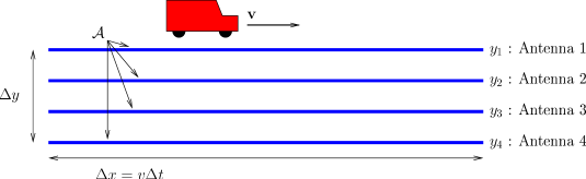
Figure 1: Four antennas mounted on a vehicle moving with velocity $v$.

Because this aperture is not a continuous curve, the results above can not applied directly. However, there is a simple argument how they can be adopted to this important case.

The problem can be solved by constructing a Hilbert space $\mathcal{H}$ on that aperture that consists of $M$ straight lines. The construction is just a slightly modified direct sum [20] of the $M$ Hilbert spaces $\mathcal{H}_{m}$, $m=1,...,M$ corresponding to these $M$ straigth lines. Let $\phi_{m},\,\psi_{m}\in\mathcal{H}_{m}$. Their scalar product is denoted as $\left\langle\phi,\psi\right\rangle_{m}$. The vectors $\phi,\,\psi\in\mathcal{H}$ are then defined as $M$-tuples $\phi=\left(\phi_{1},...,\phi_{M}\right)^{T}$, $\psi=\left(\psi_{1},...,\psi_{M}\right)^{T}$ that, for convenience, may be written as columns. Their scalar product is defined by

$$\left\langle\phi,\psi\right\rangle=\frac{1}{M}\sum_{m=1}^{M}\left\langle\phi_{m},\psi_{m}\right\rangle\,.$$ (135)

Let $\tau$ be the common priviledged parameter of all the lines. Then the scalar product can be written as

$$\left\langle\phi,\psi\right\rangle=\frac{1}{M}\sum_{m=1}^{M}\int_{0}^{1}\phi_{m}^{\ast}\left(\tau\right)\psi\left(\tau\right)\mathrm{d}\tau\,.$$ (136)

The fading process itself is a column vector $a=\left(a_{1},...,a_{M}\right)^{T}$. The corresponding autocorrelation operator $\mathbf{R}$ will then be given according to the general definition (75) as

$$\left\langle\phi,\mathbf{R}\psi\right\rangle=\mathrm{E}\left\{\left\langle\phi,a\right\rangle\left\langle a,\psi\right\rangle\right\}\,.$$ (137)

The corresponding integral kernel now becomes a tensor $\mathcal{R}_{mm^{\prime}}\left(\tau,\tau^{\prime}\right)$, $m,m^{\prime}\in\left\{1,...,M\right\}$. This kernel is a continuous matrix-valued function in $\tau$ and $\tau^{\prime}$. As a consequence of that continuity, all the results above remain valid and our method can be applied to this case.

4 Numerically calculated diversity spectra

4.1 How to Calculate Diversity Spectra

The task now is to calculate the eigenvalue spectrum according to Equation (131). It depends on the geometry of $\mathcal{A}$ and on the Fourier coefficients $\hat{s}_{n}$ of the PAS $\mathcal{S}\left(\alpha\right)$. The elements of $\mathbf{G}_{N}$ are given by $G_{mn}=\left\langle v_{m},v_{n}\right\rangle$. This scalar product is an integral over $\mathcal{A}$ and has to be calculated by numerical quadrature methods for all $m,\,n$ with $\left|m\right|,\,\left|n\right|\leq N$. The matrix elements of $\tilde{\mathbf{R}}$ are given by $\tilde{R}_{mn}=2\pi\hat{s}_{m-n}$. The truncation number $N$ governs the accuracy of the eigenvalues according to Theorem 2. For the choise $N=N_{D}+10$, e.g., the exponential is approximately $5\cdot 10^{-5}$, which can be regarded as sufficiently accurate. It is noteworthy that the constant $0.2\cdot\max_{\alpha\in\left[-\pi,\pi\right]}\left(2\pi\mathcal{S}\left(\alpha\right)\right)$ in that theorem is typically in the order of one. The number $N_{D}=\left\lceil\mathrm{e}\pi r_{1}\right\rceil$ grows with the size of the aperture $\mathcal{A}$. If, e.g., it is inside a disk with radius of one wavelength, $N_{D}=\left\lceil\mathrm{e}\pi\right\rceil=9$. Thus, for typical aperture restricted to the size of a few wavelengths, the matrices do not exceed the size of a few times ten.

4.2 The Power Azimuth Spectra

We consider two PAS prototypes that are quite popular in the literature: The uniform PAS and the von-Mises PAS.

Uniform PAS:

By this we mean a PAS that is constant over an opening angle $\Delta$. The normalised and centered uniform PAS of opening angle $\Delta$ is given by

$$\mathcal{S}\left(\alpha;\Delta\right)=\frac{1}{\Delta}\mathrm{rect}\left(\frac{\alpha}{\Delta}\right)\,.$$ (138)

The corresponding Fourier coefficients can be calculated as

$$\hat{s}_{n}=\frac{1}{2\pi}\mathrm{sinc}\left(n\frac{\Delta}{2\pi}\right)\,.$$ (139)

von-Mises PAS:

The von-Mises distribution is a circular distribution with a shape quite similar to a wrapped normal distribution [24]. Its shape is controlled by a parameter $\kappa\geq 0$, whose inverse is approximately equal to the variance of the corresponding normal distribution. The centered PAS is given by

$$\mathcal{S}\left(\alpha;\kappa\right)=\frac{1}{2\pi\mathrm{I}_{0}\left(\kappa\right)}\mathrm{e}^{\kappa\cos\alpha}\,,$$ (140)

where $\mathrm{I}_{n}\left(\kappa\right)$ denotes the modified Bessel function. The Fourier coefficients

$$\hat{s}_{n}=\frac{\mathrm{I}_{n}\left(\kappa\right)}{2\pi\mathrm{I}_{0}\left(\kappa\right)}$$ (141)

can be obtain from Formula 9.6.34 in [25].

The formulas above apply to a PAS that is centered around $\alpha=0$. The versions centered around $\alpha=\alpha_{0}$ are obtained by the shift

$$\mathcal{S}\left(\alpha\right)\mapsto\mathcal{S}\left(\alpha-\alpha_{0}\right)\,.$$ (142)

The corresponding Fourier coefficients must then be modified according to

$$\hat{s}_{n}\mapsto\hat{s}_{n}\mathrm{e}^{-j\alpha_{0}n}\,.$$

4.3 Uniform Circular Arrays

A uniform circular array (UCA) is a configuration where the antennas are mounted uniformly on a circle. In the limit of a dense array, this is just the situation of Example 1 discussed above. Figures 2 and 3 show the numerically calculated eigenvalue spectra for a ULA of radius $r=1$ (i. e. one wavelenght) for the uniform and the von-Mises PAS, respectively. The parameters $\Delta$ and $\kappa$ are adjusted manually in such a way that the corresponding values for $\omega$ are nearly identical. The eigenvalue spectra are very similar, but, however, they are not identical. Obviously, the multipath richness decreases significantly for small opening angles of the PAS, i.e. for small values of $\Delta$ and for high values of $\kappa$.

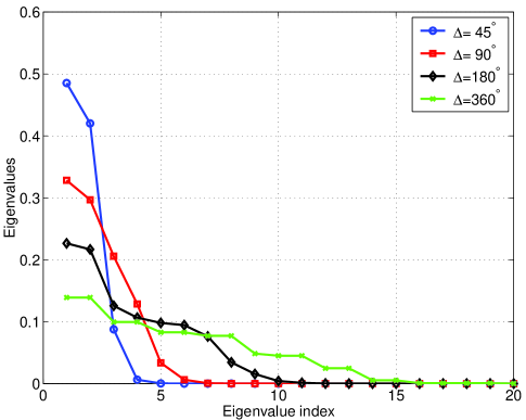
Figure 2: Diversity spectra for a dense UCA of radius $r=1$ for a uniform PAS with different opening angles $\Delta$.

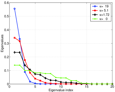
Figure 3: Diversity spectra for a dense UCA of radius $r=1$ for a von-Mises PAS with different parameters $\kappa$.

Figures 4 and 5 show $\omega$

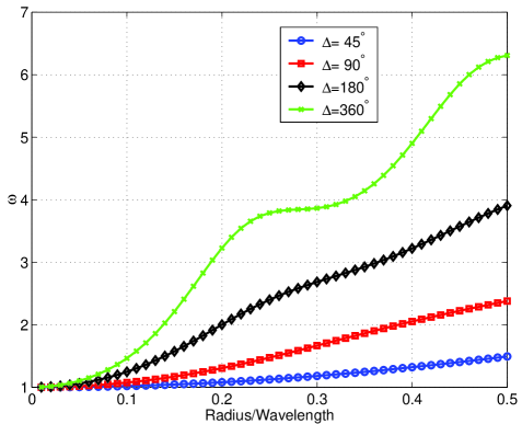
Figure 4: The diversity measure $\omega$ as a function of the radius for a dense UCA and a uniform PAS with different opening angles $\Delta$.

Figure 5: The diversity measure $\omega$ as a function of the radius for a dense UCA and a von-Mises PAS with different parameters $\kappa$.

for small radii up to $r=0.5$ for the same parameters of $\Delta$ and $\kappa$. The curves are nearly identical in both figures. The green curve of the isotropic PAS ($\Delta=360^{\circ}$ or $\kappa=0$) shows a noticable oscillatory behaviour, that can also be observed for other values that are close to the isotropic case.

4.4 Uniform Linear Arrays

For a straigth line which corresponds to a uniform linear array (ULA),

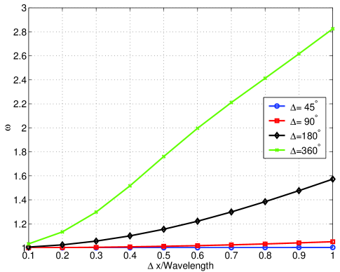
Figure 6: The diversity measure $\omega$ as a function of the size $\Delta x$ for a dense ULA and a uniform PAS with different opening angles $\Delta$. The main direction of arrival is $\alpha_{0}=0$, i.e. parallel to the array.

such an oscillatory behaviour could not be observed. Figure 6 shows $\omega$ for ULA sizes up to one wavelenght and the uniform PAS. The direction of the ULA is parallel to the mean angle of arrial ($\alpha_{0}=0$). This is the worst case, and for small values of $\Delta$ (blue and red curve), there is practically no diversity gain. Increasing the size of the ULA up to several wavelengths does not really help because the steepness of the curves is very poor. There is a strong dependency on the mean angle of arrival $\alpha_{0}$. Figure 7

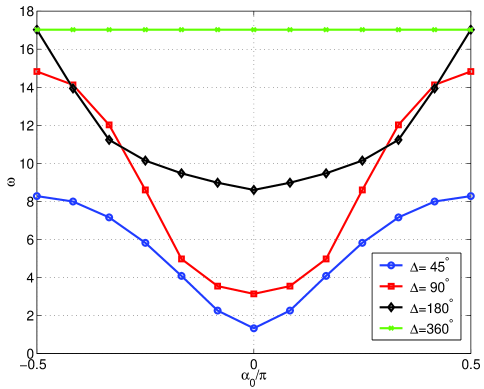
Figure 7: The diversity measure $\omega$ as a function of the main direction of arrival $\alpha_{0}$ for a dense ULA and a uniform PAS with different opening angles $\Delta$. The size of the array is $\Delta x=10$.

shows $\omega$ as a function of $\alpha_{0}$ for $\Delta x=10$. It can be seen from this figure that even for this large array, the diversity measure falls down close to one for small opening angles (blue and red curve). This means that for a narrowly focussed signal, even a huge antenna array parallel to the direction of arrival can hardly provide any diversity gain. Such narrowly focussed signal may be not very likely at the mobile station, but they will frequently occur at the base station site. Therefore it is important at that site not to fix all antennas along one line, but to distribute them in two dimensions by using, e.g., a circular array or any other two-dimensional configuration. Figure 8

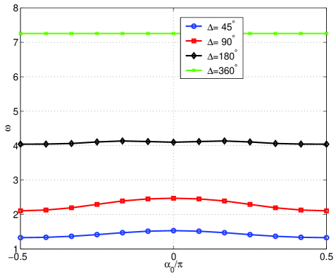
Figure 8: The diversity measure $\omega$ as a function of the main direction of arrival $\alpha_{0}$ for four parallel and equidistant lines and a uniform PAS with different opening angles $\Delta$. The length of the lines is $\Delta x=1$ and the separation of the outer lines is $\Delta y=1$.

shows $\omega$ as a function of $\alpha_{0}$ for a configuration of four parallel ULAs of length $\Delta x=1$ and a separation of the outer ULAs given by $\Delta y=1$. In that scenario, the diversity measure is very robust against rotations. As discussed above (see Figure 1), by space-time scaling $\Delta x=v\Delta t$, this situation can also be related to the scenario of a vehicle moving in x-direction with velocity $v$ and a 4-antenna communication system with time interleaving over a interval $\Delta t$.

4.5 Discrete Arrays

The focus of this paper is to analyse the diversity spectra of continuous (dense) arrays, i.e. of contiuous regions in the plane. It is interesting to compare this with the discrete case where a finite number $L$ of antennas is mounted on a finite geometrical base, i.e. a circle for the UCA or a line for the ULA. In [13], a detailed analysis has been presented how the diversity measure $\omega$ depends on the array geometry. That analysis, however, is restricted to ideal case of an isotropic PAS where the autocorrelation function is given by $\rho_{0}\left(\mathbf{x}\right)=\mathrm{J}_{0}\left(2\pi r\right)$. In the general case, the ACF is given by the expansion (28). According to Theorem 1, this can be approximated by the truncated series

$$\rho_{N}\left(\mathbf{x}\right)=\sum_{n=-N}^{N}\tilde{s}_{n}\mathrm{e}^{j\beta n}j^{n}\mathrm{J}_{n}\left(2\pi r\right)\,.$$ (143)

The appropriate order $N$ can be chosen as $N=N_{D}+10$ according to the bounds obtained in the last section. The diversity measure $\omega$ according to Equation (86) has be calculated from the matrix $\mathbf{R}$ with elements

$$R_{ik}=\rho\left(\mathbf{x}_{i}-\mathbf{x}_{k}\right)\approx\rho_{N}\left(\mathbf{x}_{i}-\mathbf{x}_{k}\right)\,,$$ (144)

where $\mathbf{x}_{i}$, $i=1,...,L$ are the antenna positions. We note that Equation (86) does not require to solve the eigenvalue problem for $\mathbf{R}$. Only the traces of the matrices $\mathbf{R}$ and $\mathbf{R}^{\dagger}\mathbf{R}$ need to be calculated.

Figure 9

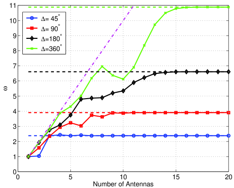
Figure 9: The diversity measure $\omega$ as a function of the number of antennas for a UCA of radius $r=1$ and a uniform PAS with different opening angles $\Delta$.

shows the depency of $\omega$ on the number $L$ of antennas for a UCA of radius $r=1$ and a uniform PAS of different opening angles $\Delta$. The margenta dash-dotted line corresponds to $\omega=L$ (i.e. the diversity measure of $L$ uncorrelated antennas). The horizontal dashed lines mark the $\omega$- values for the continuous UCA and may be interpreted as the asymptotic limit $L\to\infty$. It can be seen from the figure that for large $L$, the diversity measure runs into a saturation given by that continuous case asymptote. It is interesting to note that $\omega$ does not increase monotonically with $L$. This interesting fact has been already observed in [13] for the isotropic case (i.e. $\Delta=360^{\circ}$). In the same paper, it has also been pointed out that for a ULA, the maximal value of $\omega$ is typically reached for a relatively small number of antennas, and the limiting value for $L\to\infty$ lies below that value.

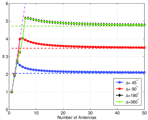
Figure 10: The diversity measure $\omega$ as a function of the number of antennas for a ULA of size $\Delta x=2$ and a uniform PAS with different opening angles $\Delta$. The signal comes from broadside ($\alpha_{0}=\pi/2$).

Figure 10 shows the situation for a ULA of size $\Delta x=2$, $\alpha_{0}=90^{\circ}$ and the same PAS parameters as above. For $\Delta=360^{\circ}$, the maximal value of $\omega$ is reached at the number of $L=6$ antenna. For $\Delta=90^{\circ}$ and $\Delta=45^{\circ}$, this number is even lower. The black curve for $\Delta=180^{\circ}$ hidden by the green curve corresponding to $\Delta=360^{\circ}$ because of the mirror symmetry of that geometrical configuration as already discussed in the context of the Doppler effect. Figure 10 (or similar figures for other values of $\Delta x$ ) provides practical design guidance for the design of linear arrays. The number of antennas should be chosen in such a way that $\omega$ is not only maximal for a special case like $\Delta=360^{\circ}$ but should stay robust against a change of the PAS.

5 Discussion and Conclusions

The diversity corresponding to an aperture $\mathcal{A}$ is characterised by the diversity spectrum $\left\{\lambda\right\}_{i=1}^{\infty}$ of eigenvalues of the spatial autocorrelation operator $\mathbf{R}$ that acts as an integral kernel on the Hilbert space of square integrable functions defined on that aperture. The diversity spectrum depends on the geometry of the aperture and the power azimuth spectrum that characterises the statistics of the spatial fading. We have shown a method for the numerical calculation solving the eigenvalue problem for an finite-dimension approximation of $\mathbf{R}$. The method provides rigorous bounds of the approximation error. A simpler, but less comprehensive characterisation compared to the whole diversity spectrum $\mathrm{eig}\left(\mathbf{R}\right)=\left\{\lambda\right\}_{i=1}^{\infty}$ is a single number named the diversity measure $\omega\left(\mathbf{R}\right)$. It can (roughly) be interpreted as the effective number of equivent independent diversity branches. Its calculation is in the same framework, but it is simpler because no eigenvalue problem has to be solved. The dependency of $\omega\left(\mathbf{R}\right)$ on the aperture geometry, on the main angle of incidence, and on the anisotropy of the PAS gives useful hints for the design of antenna arrays. For a vehicle of constant velocity moving through the spatial fading pattern, the time dependent fading can be obtained by a simple scaling, and a time interval corresponds to a spatial line segment. Therefore, the time interleaving depth for a coded system can be assigned to a line segment, and the diversity of that segment corresponds to the code diversity that can be exploited within the time interleaving depth.

Appendix A Some Definitions and Facts about linear Operators

Let $\mathbf{A}$ be a linear operator on $\mathcal{H}$. Its (hermitian) adjoint, $\mathbf{A}^{\dagger}$, is defined by

$$\left\langle\phi,\mathbf{A}^{\dagger}\psi\right\rangle=\left\langle\mathbf{A}\phi,\psi\right\rangle\,.$$ (145)

If $\mathbf{A}=\mathbf{A}^{\dagger}$ holds, the operator is called self-adjoint. In this paper, we need only to consider bounded operators. For these operator, self-adjoint is the same as the (in general weaker) property symmetric or hermitian.

A limit $\mathbf{R}_{N}\rightarrow\mathbf{R}$ for operators may be defined in different meanings. In this paper, we need three types of norms for an operator $\mathbf{A}$ on a Hilbert space $\mathcal{H}$. We briefly recall their definitions and their most important properties and refer to [20] for further details.

1. The (uniform) operator norm $\left\|\mathbf{A}\right\|$ is defined by

   $$\left\|\mathbf{A}\right\|\triangleq\sup_{\left\|\phi\right\|=1}\left\|\mathbf{A}\phi\right\|\,.$$ (146)

   Operators with $\left\|\mathbf{A}\right\|<\infty$ are called bounded operators.

2. The Hilbert-Schmidt norm $\left\|\mathbf{A}\right\|_{2}$ is defined as

   $$\left\|\mathbf{A}\right\|_{2}\triangleq\sqrt{\mathrm{tr}\left(\mathbf{A}^{\dagger}\mathbf{A}\right)}\,,$$ (147)

   where $\mathrm{tr}\left(\cdot\right)$ denotes the trace of an operator. For the special case of finite-dimensional matrices, the Hilbert-Schmidt norm is called Frobenius norm. One can show that

   $$\left\|\mathbf{A}\right\|_{2}=\sqrt{\sum_{ik}\left|A_{ik}\right|^{2}}$$ (148)

   is an equivalent definition. In that equation, $A_{ik}=\left\langle u_{i},u_{k}\right\rangle$ are the matrix elements in an arbitrary orthonormal basis $u_{i}$. Operators with $\left\|\mathbf{A}\right\|_{2}<\infty$ are called Hilbert-Schmidt operators. The Hilbert-Schmidt norm can also be written as

   $$\left\|\mathbf{A}\right\|_{2}=\sqrt{\sum_{i=1}^{\infty}\lambda_{i}^{2}}\,,$$ (149)

   where the $\lambda_{i}^{2}$ are the eigenvalues of $\mathbf{A}^{\dagger}\mathbf{A}$. In case that $\mathbf{A}$ is self-adjoint, the real numbers $\lambda_{i}$ are just the eigenvalues of $\mathbf{A}$.

3. The trace norm $\left\|\mathbf{A}\right\|_{1}$ for a self-adjoint operator is given by

   $$\left\|\mathbf{A}\right\|_{1}=\sum_{i=1}^{\infty}\left|\lambda_{i}\right|\,,$$ (150)

   where $\lambda_{i}$ are the eigenvalues of $\mathbf{A}$ and a purely discrete spectrum of $\mathbf{A}$ has been assumed. Operators with $\left\|\mathbf{A}\right\|_{1}<\infty$ are called trace class operators.

In our paper, we make use of some properties of compact operators. For the exact mathematical definition of compactness, we refer to [20]. For our purposes, it is sufficient to recall that every Hilbert-Schmidt operator is compact (see Theorem VI.22 in [20]).

From the above definitions between norms, the relation

$$\left\|\mathbf{A}\right\|_{2}^{2}=\left\|\mathbf{A}^{\dagger}\mathbf{A}\right\|_{1}\leq\left\|\mathbf{A}\right\|_{1}^{2}$$ (151)

follows immediately. Furthermore, there is the following hierarchical relation holds between the norms defined above ([20], Theorem VI.22):

$$\left\|\mathbf{A}\right\|\leq\left\|\mathbf{A}\right\|_{2}\leq\left\|\mathbf{A}\right\|_{1}$$ (152)

The following inequalities also hold

$$\left\|\mathbf{CAB}\right\|_{1}\leq\left\|\mathbf{C}\right\|\left\|\mathbf{A}\right\|_{1}\left\|\mathbf{B}\right\|\,,$$ (153)

$$\left\|\mathbf{CAB}\right\|_{2}\leq\left\|\mathbf{C}\right\|\left\|\mathbf{A}\right\|_{2}\left\|\mathbf{B}\right\|\,,$$ (154)

provided that all the norms exist.

Appendix B Proof of Theorem 2

In this appendix, we proof the bound (127) for the approximation error of the eigenvalues as stated in Theorem 2. This bound is based on bounds for approximation errors for operators.

First of all, we shall proof that the operator $\tilde{\mathbf{R}}$ with matrix elements $\tilde{R}_{mn}$ given by Equation (30) is bounded.

Lemma 1:

Under the assumption that $\mathcal{S}\left(\alpha\right)$ is a piecewise continuous, bounded function over the interval $\left[-\pi,\pi\right]$, the operator $\tilde{\mathbf{R}}$ with matrix elements $\tilde{R}_{mn}$ given by Equation (30) is bounded with operator norm given by

$$\bigl{\|}\tilde{\mathbf{R}}\bigr{\|}=2\pi\max_{\alpha\in\left[-\pi,\pi\right]}\mathcal{S}\left(\alpha\right)\triangleq\rho_{max}$$

Proof:

Since we have assumed that $\mathcal{S}\left(\alpha\right)$ is a piecewise continuous, bounded function over the interval $\left[-\pi,\pi\right]$, it defines a bounded multiplication operator

$$\mathbf{S}:\,X\left(\alpha\right)\mapsto Y\left(\alpha\right)=\mathcal{S}\left(\alpha\right)X\left(\alpha\right)$$

on $\mathcal{L}^{2}\left(\left[-\pi,\pi\right],\frac{\mathrm{d}\alpha}{2\pi}\right)$. Its operator norm is given by

$$\left\|\mathbf{S}\right\|=\max_{\alpha\in\left[-\pi,\pi\right]}\mathcal{S}\left(\alpha\right)\,.$$

The Hilbert space $\mathcal{L}^{2}\left(\left[-\pi,\pi\right],\frac{\mathrm{d}\alpha}{2\pi}\right)$ is isomorphic to the Hilbert space $\ell^{2}\left(\mathbb{Z}\right)$ of square summable sequences with indices running over $\mathbb{Z}$. The vectors $X\left(\alpha\right),\,Y\left(\alpha\right)\in\mathcal{L}^{2}\left(\left[-\pi,\pi\right],\frac{\mathrm{d}\alpha}{2\pi}\right)$ correspond to the sequences $\left\{x_{n}\right\}_{n\in\mathbb{Z}},\,\left\{y_{n}\right\}_{n\in\mathbb{Z}}\in\ell^{2}\left(\mathbb{Z}\right)$ of their Fourier coefficients. The action of the operator $\mathbf{S}$ in this discrete representation is given by the convolution

$$y_{n}=\sum_{m=-\infty}^{\infty}\hat{s}_{m-n}x_{n}\,,$$

where $\hat{s}_{n}$ are the Fourier coefficients of $\mathcal{S}\left(\alpha\right)$. Comparing with Equation (30) we see that $\tilde{\mathbf{R}}=2\pi\mathbf{S}$ holds in this represention. Since the operator norm does not depend on the representation, we conclude that $\bigl{\|}\tilde{\mathbf{R}}\bigr{\|}=2\pi\left\|\mathbf{S}\right\|$, which completes the proof. $\blacksquare$

For two compact and self-adjoint operators, the difference of the corresponding eigenvalues is bounded by the operator norm of their difference. We cite the following fact from the textbook of Riesz and Nagy [22], § 95:

Lemma 2:

Let $\mathbf{A}$ and $\mathbf{B}$ be self-adjoint compact operators and define

$$\mathbf{C=A+B}\,.$$

Assume that the eigenvalues $\lambda_{i}\left(\mathbf{A}\right)$ of $\mathbf{A}$ and $\lambda_{i}\left(\mathbf{C}\right)$ of $\mathbf{C}$ are ordered according to (129). Then their difference is bounded by

$$\left|\lambda_{i}\left(\mathbf{C}\right)-\lambda_{i}\left(\mathbf{A}\right)\right|\leq\left\|\mathbf{B}\right\|\,$$

for all $i$.

Corolarry to Lemma 2:

Setting $\mathbf{C}=\mathbf{R}$, $\mathbf{A}=\mathbf{R}_{N}$, and $\mathbf{B}=\mathbf{R}-\mathbf{R}_{N}$ leads to the inequality

$$\left|\lambda_{i}\left(\mathbf{R}\right)-\lambda_{i}\left(\mathbf{R}_{N}\right)\right|\leq\left\|\mathbf{R}-\mathbf{R}_{N}\right\|$$ (155)

The goal now is to show that $\left\|\mathbf{R}-\mathbf{R}_{N}\right\|\to 0$ holds for $N\to\infty$.

In the following, we assume that $\mathcal{A}\subset\mathcal{D}$, where $\mathcal{D}$ is a disk of radius $r_{1}$. We define $N_{D}=\left\lceil\mathrm{e}\pi r_{1}\right\rceil$ and assume that $N\geq N_{D}$.

The transformation matrix $\mathbf{T}$ is defined by its elements $T_{mn}=\left\langle u_{m},v_{n}\right\rangle$. The Gram matrix $\mathbf{G}=\mathbf{T}^{\dagger}\mathbf{T}$ has matrix elements $G_{mn}=\left\langle v_{m},v_{n}\right\rangle$. The squared Hilbert-Schmidt norm of $\mathbf{T}$ is given by

$$\left\|\mathbf{T}\right\|_{2}^{2}=\left\|\mathbf{T}^{\dagger}\mathbf{T}\right\|_{1}=\left\|\mathbf{G}\right\|_{1}=\sum_{n=-\infty}^{\infty}\left\langle v_{n},v_{n}\right\rangle\,.$$ (156)

Using Equation (97) we may write

$$\left\langle v_{n},v_{n}\right\rangle = \int_{\mathcal{A}}\left|v_{n}\left(\mathbf{x}\right)\right|^{2}\mathrm{d}\mu\left(\mathbf{x}\right)\,.$$

$$= \int_{\mathcal{A}}\mathrm{J}_{n}^{2}\left(2\pi\left|\mathbf{x}\right|\right)\mathrm{d}\mu\left(\mathbf{x}\right)$$

The integral is over the array $\mathcal{A}$ with $\mathrm{d}\mu\left(\mathbf{x}\right)$ given by Equation (54) or (65) for the respective cases. Inserting the above expression into Equation (156) leads to

$$\left\|\mathbf{T}\right\|_{2}^{2} = \int_{\mathcal{A}}\sum_{n=-\infty}^{\infty}\mathrm{J}_{n}^{2}\left(2\pi\left|\mathbf{x}\right|\right)\mathrm{d}\mu\left(\mathbf{x}\right)\,.$$

The properties

$$\sum_{n=-\infty}^{\infty}\mathrm{J}_{n}^{2}\left(x\right)=1$$

and

$$\int_{\mathcal{A}}\mathrm{d}\mu\left(\mathbf{x}\right)=1$$

then yield

$$\left\|\mathbf{T}\right\|_{2}^{2}=1\,.$$ (157)

We now define a truncated transformation matrix $\mathbf{T}_{N}$ that has the same matrix elements as $\mathbf{T}$ inside the middle square defined by $\left|m\right|\leq N$ and $\left|n\right|\leq N$. All other matrix elements are set to zero. The remainder matrix $\mathbf{T}-\mathbf{T}_{N}$ has only non-vanishing matrix elements outside that middle square. Its squared Hilbert-Schmidt norm is given by

$$\left\|\mathbf{T}-\mathbf{T}_{N}\right\|_{2}^{2} = \mathrm{tr}\left[\left(\mathbf{T}-\mathbf{T}_{N}\right)^{\dagger}\left(\mathbf{T}-\mathbf{T}_{N}\right)\right]$$

$$= \mathrm{tr}\left(\mathbf{T}^{\dagger}\mathbf{T}+\mathbf{T}_{N}^{\dagger}\mathbf{T}_{N}-\mathbf{T}^{\dagger}\mathbf{T}_{N}-\mathbf{T}_{N}^{\dagger}\mathbf{T}\right)$$

$$= \mathrm{tr}\left(\mathbf{T}^{\dagger}\mathbf{T}\right)+\mathrm{tr}\left(\mathbf{T}_{N}^{\dagger}\mathbf{T}_{N}\right)-\mathrm{tr}\left(\mathbf{T}^{\dagger}\mathbf{T}_{N}\right)-\mathrm{tr}\left(\mathbf{T}_{N}^{\dagger}\mathbf{T}\right)$$

$$= \mathrm{tr}\left(\mathbf{T}^{\dagger}\mathbf{T}\right)-\mathrm{tr}\left(\mathbf{T}_{N}^{\dagger}\mathbf{T}_{N}\right)$$

$$= \mathrm{tr}\left(\mathbf{T}^{\dagger}\mathbf{T}-\mathbf{T}_{N}^{\dagger}\mathbf{T}_{N}\right)$$

Here we have used the fact that $\mathbf{T}^{\dagger}\mathbf{T}_{N}=\mathbf{T}_{N}^{\dagger}\mathbf{T}_{N}$ and thus $\mathrm{tr}\left(\mathbf{T}^{\dagger}\mathbf{T}_{N}\right)=\mathrm{tr}\left(\mathbf{T}_{N}^{\dagger}\mathbf{T}_{N}\right)$. The truncated Gram matrix $\mathbf{G}_{N}=\mathbf{T}_{N}^{\dagger}\mathbf{T}_{N}$ has the same matrix elements as $\mathbf{G}$ inside the inner square and zero elements outside. Thus, the expression derived above can be written as

$$\left\|\mathbf{T}-\mathbf{T}_{N}\right\|_{2}^{2} = \mathrm{tr}\left(\mathbf{G}-\mathbf{G}_{N}\right)$$

$$= \sum_{\left|n\right|>N}\left\langle v_{n},v_{n}\right\rangle$$

$$= \int_{\mathcal{A}}\sum_{\left|n\right|>N}\mathrm{J}_{n}^{2}\left(2\pi\left|\mathbf{x}\right|\right)\mathrm{d}\mu\left(\mathbf{x}\right)$$

From Theorem 1 we get the bound

$$\left\|\mathbf{T}-\mathbf{T}_{N}\right\|_{2}^{2}\leq 0.01\,\exp\left[2\left(N_{D}-N\right)\right]\,.$$

Taking the square root yields

$$\left\|\mathbf{T}-\mathbf{T}_{N}\right\|_{2}\leq 0.1\,\exp\left(N_{D}-N\right)\,.$$ (158)

From

$$\left\|\mathbf{T}_{N}\right\|_{2}^{2}=\sum_{\left|n\right|\leq N}\left\langle v_{n},v_{n}\right\rangle$$

and Equations (156) and (157) we conclude that

$$\left\|\mathbf{T}_{N}\right\|_{2}\leq\left\|\mathbf{T}\right\|_{2}=1\,$$ (159)

holds. We define the truncated correlation matrix

$$\mathbf{R}_{N}=\mathbf{T}_{N}\tilde{\mathbf{R}}\mathbf{T}_{N}^{\dagger}\,.$$ (160)

The Hilbert-Schmidt norm approximation error relative to $\mathbf{R}=\mathbf{T}\tilde{\mathbf{R}}\mathbf{T}^{\dagger}$ can now be estimated as follows:

$$\left\|\mathbf{R}-\mathbf{R}_{N}\right\|_{2} = \left\|\mathbf{T}\tilde{\mathbf{R}}\mathbf{T}^{\dagger}-\mathbf{T}_{N}\tilde{\mathbf{R}}\mathbf{T}_{N}^{\dagger}\right\|_{2}$$

$$= \left\|\mathbf{T}\tilde{\mathbf{R}}\left(\mathbf{T}-\mathbf{T}_{N}\right)^{\dagger}+\left(\mathbf{T}-\mathbf{T}_{N}\right)\tilde{\mathbf{R}}\mathbf{T}_{N}^{\dagger}\right\|_{2}$$

$$\leq \left\|\mathbf{T}\tilde{\mathbf{R}}\left(\mathbf{T}-\mathbf{T}_{N}\right)^{\dagger}\right\|_{2}+\left\|\left(\mathbf{T}-\mathbf{T}_{N}\right)\tilde{\mathbf{R}}\mathbf{T}_{N}^{\dagger}\right\|_{2}$$

$$\leq \left\|\mathbf{T}\right\|_{2}\bigl{\|}\tilde{\mathbf{R}}\bigr{\|}\left\|\mathbf{T}-\mathbf{T}_{N}\right\|_{2}+\left\|\mathbf{T}-\mathbf{T}_{N}\right\|_{2}\bigl{\|}\tilde{\mathbf{R}}\bigr{\|}\left\|\mathbf{T}_{N}\right\|_{2}$$

$$\leq 2\bigl{\|}\tilde{\mathbf{R}}\bigr{\|}\left\|\mathbf{T}-\mathbf{T}_{N}\right\|_{2}$$

From the bound (158) we conclude

$$\left\|\mathbf{R}-\mathbf{R}_{N}\right\|_{2}\leq 0.2\cdot\bigl{\|}\tilde{\mathbf{R}}\bigr{\|}\exp\left(N_{D}-N\right)\,.$$ (161)

The norm hierarchy (152) yields

$$\left\|\mathbf{R}-\mathbf{R}_{N}\right\|\leq 0.2\cdot\bigl{\|}\tilde{\mathbf{R}}\bigr{\|}\exp\left(N_{D}-N\right)\,.$$ (162)

From the Corollary to Lemma 2 we obtain

$$\left|\lambda_{i}\left(\mathbf{R}\right)-\lambda_{i}\left(\mathbf{R}_{N}\right)\right|\leq 0.2\cdot\left\|\tilde{\mathbf{R}}\right\|\exp\left(N_{D}-N\right)\,.$$

Lemma 1 then leads to Theorem 2.

Appendix C Proof of Theorem 3

In this appendix, we prove the bound (133) for the approximation error of the squared Hilbert Schmidt norms as stated in Theorem 3. From $\mathbf{R}=\mathbf{T}\tilde{\mathbf{R}}\mathbf{T}^{\dagger}$ and $\mathbf{R}_{N}=\mathbf{T}_{N}\tilde{\mathbf{R}}\mathbf{T}_{N}^{\dagger}$ and Inequality (159) we conclude

$$\left\|\mathbf{R}\right\|_{2}\leq\bigl{\|}\tilde{\mathbf{R}}\bigr{\|}\mbox{ and }\left\|\mathbf{R}_{N}\right\|_{2}\leq\bigl{\|}\tilde{\mathbf{R}}\bigr{\|}\,.$$

Then

$$\left|\left\|\mathbf{R}\right\|_{2}^{2}-\left\|\mathbf{R}_{N}\right\|_{2}^{2}\right| = \Bigl{|}\left\|\mathbf{R}\right\|_{2}-\left\|\mathbf{R}_{N}\right\|_{2}\Bigr{|}\left(\left\|\mathbf{R}\right\|_{2}+\left\|\mathbf{R}_{N}\right\|_{2}\right)$$

$$\leq 2\bigl{\|}\tilde{\mathbf{R}}\bigr{\|}\Bigl{|}\left\|\mathbf{R}\right\|_{2}-\left\|\mathbf{R}_{N}\right\|_{2}\Bigr{|}$$

The bound (161) yields

$$\left|\left\|\mathbf{R}\right\|_{2}^{2}-\left\|\mathbf{R}_{N}\right\|_{2}^{2}\right|\leq 0.4\bigl{\|}\tilde{\mathbf{R}}\bigr{\|}^{2}\exp\left(N_{D}-N\right)\,.$$

With Lemma 1 we then obtain Theorem 3.

References

- [1] J. G. Proakis and M. Salehi, Digital Communications. McGraw-Hill, fifth ed., 2008.
- [2] S. Benedetto and E. Biglieri, Principles of Digital Transmission With Wireless Applications. Kluwer, 1999.
- [3] T. S. Rappaport, Wireless Communications: Principles and Practice. Prentice Hall, second ed., 2001.
- [4] H. Schulze and C. Lüders, Theory and Practice of OFDM and CDMA - Wideband Wireless Communications. Wiley, 2005.
- [5] G. Foschini and M. Gans, “On limits of wireless communications in a fading environment when using multiple antennas,” Wireless Personal Communications, vol. 6, pp. 311–335, March 1998.
- [6] I. E. Telatar, “Capacity of multi-antenna Gaussian channels,” European Transactions on Telecommunications, vol. 10, pp. 585–595, December 1999.
- [7] V. Kühn, Wireless Communications over MIMO Channels: Applications to CDMA and Multiple Antenna Systems. Wiley, 2006.
- [8] H. Van Trees, Detection, estimation, and modulation theory, Part I. Wiley, 2001.
- [9] W. B. Davenport and W. Root, An Introduction to the theory of random signals and noise. McGraw-Hill, 1958.
- [10] A. Papoulis, Probability, Random Variables, and Stochastic Processes. McGraw-Hill, 1991.
- [11] H. Schulze, “Matched filter bounds for multi-antenna OFDM systems,” in Proc. 15 th Int. OFDM Workshop (Hamburg), 2010.
- [12] M. T. Ivrlač and J. A. Nossek, “Quantifying diversity and correlation in Rayleigh fading MIMO communication systems,” in International Symposium on Signal Processing and Information Theory, 2003.
- [13] T. Muharemovic, A. Sabharwal, and B. Aazhang, “Antenna packing in low-power systems: Communication limits and array design,” IEEE Trans. Inform. Theory, vol. IT-54(1), pp. 429–440, January 2008.
- [14] A. Lozano, A. M. Tulino, and S. Verdu, “Multiple-antenna capacity in the low-power regime,” IEEE Trans. Inform. Theory, vol. IT-49(10), pp. 2527–2544, October 2003.
- [15] R. A. Kennedy, P. Sadeghi, T. D. Abhayapala, and H. M. Jones, “Intrinsic limits of dimensionality and richness in random multipath fields,” IEEE Trans. on Signal Processing, vol. 55 (6), pp. 2542–2556, June 2007.
- [16] G. B. Arfken and H. J. Weber, Mathematical Methods for Physicists. Elsevier, 6th ed., 2005.
- [17] P. A. Bello, “Characterization of randomly time-variant linear channels,” IEEE Trans. Commun. Syst., vol. CS-11, pp. 360–393, Dec. 1963.
- [18] B. H. Fleury, “First- and second-order characterization of direction dispersion and space selectivity in the radio channel,” IEEE Trans. Inf. Theory, vol. 46(6), pp. 2027–2047, September 2000.
- [19] W. C. Jakes, Microwave Mobile Communications. Wiley-Interscience, 1974.
- [20] M. Reed and B. Simon, Methods of modern mathematical physics, Vol. 1: Functional Analysis. Academic Press, 1980.
- [21] R. Courant and D. Hilbert, Methoden der Mathematischen Physik, Bd. 1. Springer-Verlag, 1968.
- [22] F. Riesz and B. Sz.-Nagy, Functional Analysis. Dover, 1990.
- [23] R. A. Horn and C. R. Johnson, Matrix Ananlysis. Cambridge, 1985.
- [24] P. Ravindran, Bayesian Analysis of Circular Data Using Wrapped Distributions. Dissertation, North Carolina State University, 2002.
- [25] M. Abramowitz and I. Stegun, Handbook of Mathematical Functions. Dover, 1964.