Mapping forces in 3D elastic assembly of grains.

Abstract

Our understanding of the elasticity and rheology of disordered materials, such as granular piles, foams, emulsions or dense suspensions relies on improving experimental tools to characterize their behaviour at the particle scale. While 2D observations are now routinely carried out in laboratories, 3D measurements remain a challenge. In this paper, we use a simple model system, a packing of soft elastic spheres, to illustrate the capability of X-ray microtomography to characterise the internal structure and local behaviour of granular systems. Image analysis techniques can resolve grain positions, shapes and contact areas; this is used to investigate the material’s microstructure and its evolution upon strain. In addition to morphological measurements, we develop a technique to quantify contact forces and estimate the internal stress tensor. As will be illustrated in this paper, this opens the door to a broad array of static and dynamical measurements in 3D disordered systems.

Despite the practical importance of macroscopic disordered materials such as soil, foams and emulsions the rules that govern their mechanical behaviour remain poorly understood. In the case of granular materials, these studies are essential to the advancement of related industrial processes and also to the prediction of often catastrophic geological phenomena (avalanches of slurries, earthquakes). Although empirical constitutive equations are nowadays able to partly model the response of these systems, a unified multiscale framework does not exist yet. Over the past 20 years, foams and granular systems have emerged as a model system for low temperature glasses Langer:00 . Many theories and experiments have been designed to address the relationship between the internal structure and macroscopic behaviour of such systems. These theories and models often use approaches derived from statistical physics Zhang:05a ; OHern:01 . Although the behaviour of foams seems today rather well understood Weaire2010 , the complexity of granular matters behaviour at the microscopic scale has prevented a proper physical model of granular systems. A large part of the problem arises from the strongly nonlinear contact law between rigid bodies coupled with the dynamical nature of the contact network. In this context, the spatial distribution and temporal evolution of the force network has become a highly sought after quantity that expands from micro scale (grain-grain contacts) to macro scale (granular assembly).

Early simulations have provided important insights on the internal force distributions of a granular pile Radjai:96 ; Coppersmith:96 ; Makse:00a . Two-dimensional (2D) experiments managed to keep up with the pace of advancement in simulations Drescher:72 ; Howell:99 ; Kolb:04 , 3D experiments however, have been limited to measurements of the distribution of forces only at the boundaries of the containers Brockbank:97 ; Mueth:98 ; Blair:01 ; Corwin:05 . These experimental methods could not have access to the spatial arrangement of the contact force network in the bulk of granular assemply. Moreover they were unable to determine structural features such as force chains and arching which have been postulated as the signature of jamming Lois:07 .

In recent years, a range of tools have been developed to apprehend the 3D nature of bulk properties. X-ray or MRI techniques have allowed to study dynamic properties of granular systems such as flow profiles and shear banding, at a mesoscopic scale Mantle:01 ; Alex:05 ; Alex:09 ; Dijksman:10 . 3D reconstructions of compressed emulsion systems using confocal microscopy have provided the first measurements of the bulk force distributions Brujic:03 ; Bruji:05 by estimating the contact force from contact geometry. A similar technique has also been used to characterise spatial correlations of forces inside 3D piles of frictionless liquid droplets Zhou06 . Although these observations are very valuable, the systems used are significantly different from real granular pile which has very different contact laws and frictional properties.

X-ray computed tomography has been used for static characterisation of large packings of spherical grains Silb:02 ; Aste:05 ; saadatfarthesis . In this study, we apply this technique to a model system made of soft millimetric elastic beads. In addition to the measurement of traditional structural quantities (packing fraction, coordination number etc.), the contact force is measured from the contact area between grains which can be integrated at a mesoscopic scale to estimate the local stress tensor in the pile. We then apply a series of external forces to our model system and investigate its response to these controlled loadings. This approach delivers results consistent with the existing literature and is promising as a generic tool to study the local, non-linear mechanics of granular assemblies.

1 Experiment and methodology

1.1 Experimental setup

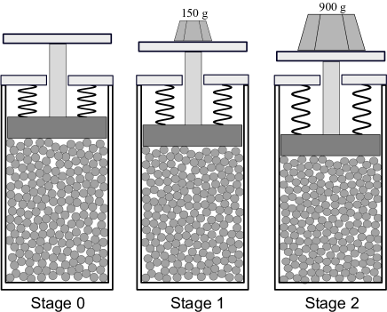
Figure 1: Sketch of the compression cell and consecutive stages of compression.

The packing studied in this paper is made of relatively monodisperse spherical rubber balls of diameter $3.10\pm 0.05~{}mm$ . The maximum and minimum ball diameter measured in the packing are $3.19mm$ and $2.85mm$ respectively. The grains are made of commercial rubber with a shear modulus estimated at $850kPa$ .

A cylindrical PMMA container, with internal diameter of $44mm$ is used as a compression cell (see figure 1). The inner wall of the cylinder is lubricated with canola oil to reduce the friction. $2020$ rubber elastic balls are then poured into this chamber. The latter is then closed at the top by a piston of diameter slightly smaller than the container; it can therefore move freely without touching the PMMA cylinder and without allowing beads to leave the container. A horizontal platform is rigidly connected by a shaft to the piston so that a load can be applied to the sample by placing weights on it. A pair of springs connecting the piston to the container is used to make sure that, in the absence of a load, the piston does not fall down due to its own weight.

The compression cell is attached to a motorised rotation stage located between a high-resolution microfocus X-ray source ($80kV$ accelerating voltage and $200\mu A$ beam current and a CCD detector of the size $67mm\times 67mm$, $2048\times 2048$ pixels of size $33.6\mu m$ each Arthur:04a ; Arthur:04b . The compression cell is rotated by about $0.125$ degree increments around its vertical axis and a radiographic projection of the packing is taken after each rotation with an exposure time of $18$ s. A total of $2880$ projections are taken for a complete rotation of the specimen. It takes approximately $15$ hours to scan the volume for each case. After the completion of each scan, tomographic cone beam reconstructions are performed on these $2880$ projections using the a Feldkamp algorithm Feldkamp84 . Tomograms of about $2000^{3}$ voxels are obtained at $27$ microns resolutions.

We have recorded and analysed the internal geometry of the packing under three different loading conditions.

Stage 0:

Pre-compression stage with no extra loading; the piston is held in balance just above the top of the packing without making contact with it (see Fig. 1). Rubber balls are at rest, only bearing their own weight ($41.1g$). The combined weight of the piston and the platform ($600g$) is fully balanced by the pull of the springs so that at this point there is no external force being exerted onto the pile.

Stage 1:

The platform is loaded with $150g$($1.47N$). By taking into account the opposite force applied by the springs, a net weight of $115g$ is applied to the packing, resulting in a compressive strain of $\epsilon=3.78\%$. We define the axial strains as the ratio of the displacement of piston to the initial height of the packing (engineering strains).

Stage 2:

A total of $900g$($8.83N$) is placed on the platform resulting in a net $780g$ weight onto the packing. The total axial strain at that stage is $\epsilon=7.83\%$.

1.2 3D Image analysis: segmentation and partitioning

The tomographic image consists of a cubic array of reconstructed linear X-ray attenuation coefficient values, each corresponding to a finite volume cube (voxel) of the sample. The first step in analysing this data is to differentiate the attenuation map into distinct pore and grain phases. Ideally, one would wish to have a bi-modal distribution giving unambiguous phase separation of the pore and solid phase peaks. This simple phase extraction is possible in our rubber ball pack. The intensity histogram of the tomogram (Fig. 2(a)) shows two distinct peaks associated with the two phases (beads and air). The peak centred around $9000$ is associated with the beads and the lower peak around $4000$ is associated with the pore phase.

(a)

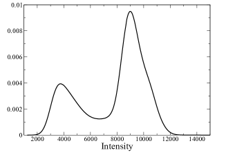
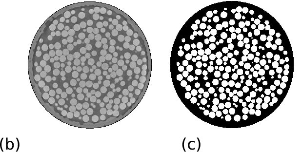
Figure 2: (a) Normalized X-ray density histogram of the full image volume of the rubber ball sample. (b) Gray scale X-ray density map of a slice of rubber ball sample. (c) The same slices after phase separation.

The segmentation algorithm Adrian:04 uses both the attenuation value and its gradient to detect interfaces between the two phases (grain-void). In particular, a sharp gradient of attenuation is required to detect an interface. This method, after adjustment Saadatfar:06 , provides a very robust detection of grain boundaries, but is of course limited to void spaces larger than the voxel size. In particular, if the gap between two grains is very small (order of a voxel), the density gradient across the gap between these two grains will not appear as steep as a typical grain-void interface. This can result in the detection of false contact regions in the segmented datasets which consequently gives rise to the following undesired morphological effects: i) detection of false contacts between grains, and ii) the surface area of real contacts appear larger than their actual values. As detailled later in this paper, this effect can be corrected in spherical grain piles by offsetting the apparent contact area of the grains.

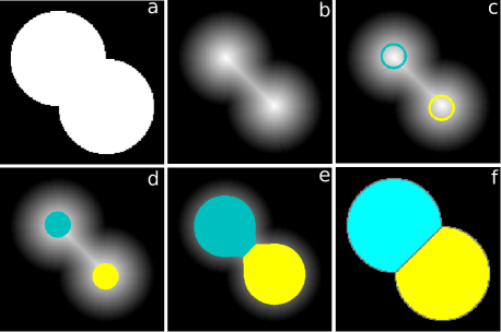
Figure 3: Different stages of the watershed algorithm. (a) Two overlapping discs. (b) EDT of the two overlapping discs. (c) Identifying the local maxima (seeds). (d) and (e) Regions grow from the initial seeds by having pixels on their boundary added to them. (f) Discs separated.

The next step is to reconstruct and label individual grains from the geometry of the solid phase. The basic assumption in the grain identification algorithm is that the boundaries between grains which are not isolated coincide with the watershed surfaces of the Euclidean distance map of grains (distance to the nearest grain boundary) Vincent:91 . The entire grain space can be thought of as the union of spheres centred on every grain voxel. Each sphere radius is given by the Euclidean distance value of the voxel at its centre. The next stage is identifying all the voxels that are not covered by any larger Euclidean spheres.

Each one of these voxels, which are at the maxima of the distance function in their local neighbourhood, then forms a seed that will grow into a single grain in the following stage of the algorithm. Fig. 3 illustrates a simple 2D case where 2 overlapping discs are separated. The seed regions essentially grow by having voxels on their boundary added to them. Voxels that lie on the boundaries of the regions are processed in reverse Euclidean distance order, i.e. voxels with high distance values are processed first. When a voxel is processed, it is assigned to the region on whose boundary it lies, or, if it lies on more than one region boundary, the region whose boundary it first became part of. At the end of the algorithm, the grain space will be partitioned into grains whose boundaries lie on the watershed surfaces of the Euclidean distance function saadatfarthesis . The watershed based grain partitioning algorithm is computationally expensive. Hence it is parallelised (using an implementation of the ”time warp” discrete event simulation protocol Soille:03 ), so it can be used to analyse very large datasets ($\sim 2000^{3}$).

2 Measurements

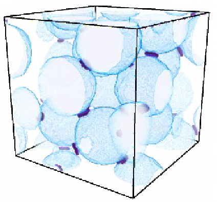
Figure 4: A subvolume of the elastic ball compaction experiment. The contact zone between touching grains (dark patches) provides a measurement of contact force.

The 3D watershed algorithm provides us with large amounts of information about the pile structure. Each grain has been labelled, its location and shape are known, its direct neighbours have been identified, and the geometry of the contact they share can been extracted as well. This data can now be processed to extract physical and mechanical properties. In this section, we present a few methods implemented in the context of granular systems. These can be separated into structural characteristics and mechanical measurements. The latter involves kinematic and force measurements that rely on prior knowledge of a contact law for individual grains.

2.1 Structural quantities

2.1.1 Packing fraction

One of the most readily measurable quantities from 3D images is the packing fraction. Packing fraction or apparent density is defined as the ratio of the volume of balls to the total volume. Table 1 summarises the packing fractions measured directly from the digital images. The packing fractions we measure on the initial pile is $57\%$, which is in the lower end of the spectrum for monodisperse beads. Such a density is achievable in our system due to the large frictional coefficient of rubber-rubber contacts. As the loading is increased, the volume fraction increases up to $62\%$.

Compression stage	$0$	$1$	$2$
Loading [gr]	$0$	$115$	$780$
Strain [%]	$0$	$3.78$	$7.83$
Packing fraction	$0.57$	$0.59$	$0.62$
Avg. coord. no.	$6.28\pm 1.64$	$6.63\pm 1.58$	$7.13\pm 1.49$
raw
Avg. coord. no.	$4.99\pm 1.80$	$5.32\pm 1.66$	$5.92\pm 1.56$
filtered

Table 1: Details of the compression progression.

2.1.2 Radial Distribution Function

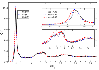
Figure 5: Autocorrelation function of the packing at different stages of compression normalized by the volume of a single grain and the packing fraction. Note the shift in the peaks as the pressure increases.

From the shapes of the individual grains calculated by the Watershed algorithm, the coordinates of each grain’s centre of mass can be accurately measured. This data is in particular required to characterize the microstructure of granular systems and to calculate the autocorrelation function of the grain centres.

The radial distribution function (RDF) is a measure of the degree of separation of grain centres and their density at a given distance. It is calculated by counting the number of grains $N$ that are separated from a given sphere by a distance in the interval $[r,r+dr]$, where $r$ is the distance between grain centres. For large $r$ the number density of the grain centres found in the interval $[r,r+dr]$ approaches the average density of grains in the packing, $\frac{3}{4\pi{R}^{3}}\rho$, where $\rho$ is the packing fraction and $R$ is average grain radius. In our calculations, we normalize RDF by the average density. Figure 5 shows the RDF in our packings throughout compression progression. The RDF of the system before insertion of any external force (stage 0) shows a prominent peak at $r\approx D_{g}$ where $D_{g}$ is the average grain diameter ($D_{g}=2\times R\approx 3.10mm$). The second peak appears at $r\approx 1.95D_{g}$ and a sub-peak approximately at $r=\sqrt{3}D_{g}$. As the vertical load increases (stage 1 and stage 2), the peak of the RDF widens and shifts to the left due to the compression of touching spheres, hence shortening the centre-centre distance between them (see Fig. 5(left)).

(a)
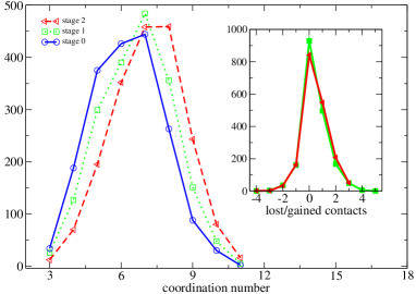
(b)

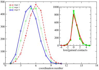
Figure 6: Histogram of coordination number as a function of loading for different threshold values: (a) No threshold is applied (using the raw data after watershed algorithm). (b) After a threshold value of $0.35~{}mm^{2}$ is subtracted from all contact surface areas. As a result the average coordination number is reduced in all three stages.

The magnitude of the shift is about $1\%$ and $2\%$ for stages $1$ and $2$. This is to be compared with the macroscopic axial strain which is of the other of 4% and 8% without any deformation along the order directions. This suggests that the internal compression is more isotropic than the loading.

2.1.3 Mean coordination

The grain partitioning also provides us with the list of contact areas between grains, from which it is possible to analyze the contact network of grains. Using first the raw data from the watershed algorithm, we have measured the coordination (number of contacts) of each grain and plotted its distribution for each stage of compression (see Figure 6(a)). This plot shows a significant increase of grain coordination as the loading increases. It is notable that as pressure increases, the distributions move to higher values and get slightly narrower (see Table 1). This increase in the coordination number is achieved by re-organisation of grains in the packing when they are compressed and also grain compression/deformation process which reduces the overall grain-grain distance. A relatively large number of grains lose their contacts with some of their immediate neighbours while almost the same amount gain new contacts as the compression progresses. We have shown the histogram of lost/gained contacts in the inset of figure 6. Negative values on the horizontal axis represent lost contacts while positive values show the number of newly gained contacts. Nearly $50\%$ of grains retain their coordination number during the compression without any changes.

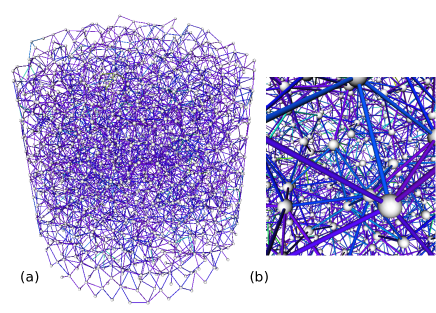
Figure 7: (a) Network representation the full packing. (b) An internal view of the packing illustrating the connecting grains

As discussed in section 3, the inherent finite resolution of the CT leads to systematic bias in fine details such as grain contacts; if the gap between two grains is in the order of, or less than, the voxel size, grains will appear to be in contact in the segmented data. To correct for this intrinsic resolution limitation, we offset all the contact areas by a small amount, which essentially corresponds to the apparent contact area of two touching perfectly spherical grains (see section 2.2.3 for detailed discussion). All contacts whose apparent surface area is below this threshold, are therefore discarded. Figure 6(b) shows a re-plot of figure 6(a) after applying the offset. The isostatic limit for mechanically stable packing of spheres in 3D suggests a connectivity of $4$ for frictional and $6$ for frictionless systems. In our measurements, the average coordination number is $\simeq 5$ for stage $0$ (see Fig.6(b)) which is in agreement with previous measurements bernal:60 ; Aste:05 .

From the knowledge of the whole contact network, a large number of other morphological and topological quantities can be calculated, such as spatial correlations in contact orientations, or contact anisotropy. Figure 7 shows a reconstruction of the contact network through which forces propagate. The statistical properties of such networks will be developed in further studies. In what follows, we will focus on the determination of mechanical forces within the pile, at the micro scale, as well as mesoscopic scale.

2.2 Kinematics and dynamics

2.2.1 Displacement fields

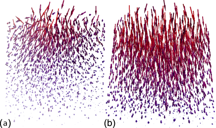
Figure 8: Displacement field presented as vector fields (velocity fields) for stage 1 (a) and 2 (b) of the experiment.

We calculate next the coordinates of the centroid of the grains for all three scans and then track each individual grain throughout the experiment. As an illustration, we render the 3D vector field derived from tracking grains during the compression for both stages of compression, see figures 8(a-b).

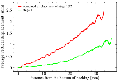
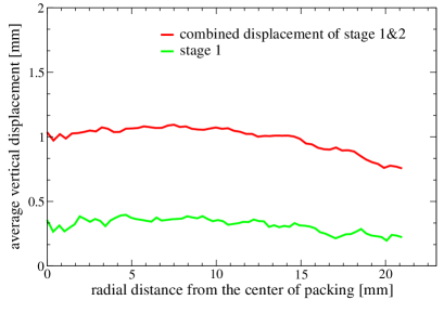
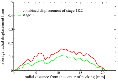
(a) (b) (c)

Figure 9: Displacement field along the loading axis. (a) The overall vertical displacement field is represented very well by an exponential equation. For visual convenience every 30 data points is shown. (b) Longitudinal displacement for the 1st stage and the overall displacement. Here we choose a bin size of $0.4mm$ for averaging. (c) Average radial displacement of grains measured from the distance between the centre of packing its outer boundary.

To gain a qualitative insight into the displacement field, we measure the average displacement of grain centres in both longitudinal and radial directions. Figure 9(a) demonstrates such displacement along the loading axis. As expected, gradient of displacement from top to bottom shows that the system is under vertical compression. The decrease of the slope with depth also indicates that part of this stress is screened by the time it reaches the bottom. A typical explanation of this is the Janssen effect Janssen:1895 , suggesting that friction on the lateral walls might be significant. To confirm this, we studied the vertical displacement profile in the radial direction (figure 9(b)) which confirms that grain movements closer to the outer region of cylinder are smaller than that of the central region. Therefore a shear component in the $(z,r)$ direction is expected. Another feature of the displacement field is the weak but noticeable radial displacement of the grain towards the boundary (see figure 9(c)). This radial displacement can be clearly seen in figure 8(a).

2.2.2 Contact mechanics

In addition to the direct measurement of individual grain displacements, a number of other mechanically relevant features can be extracted from the tomogram. Upon compression, we observed that the distance between grains varies, as well as shape and contact areas between grains. These quantities can a priori be used to quantify the force transmitted between the grains. In this section, we describe the implementation of a contact model that is suitable for stress calculations from 3D images.

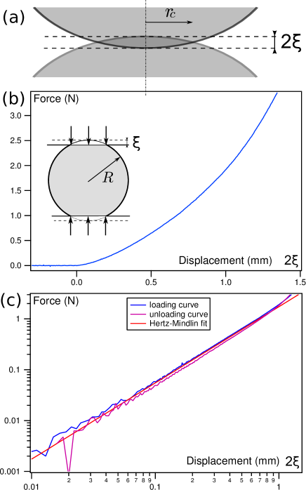
Figure 10: Response of a single rubber ball to loading.

Contact mechanics between solid objects have been studied for over a century. The seminal works of Hertz Hertz:1882 and Mindlin Mindlin:49 about the contact mechanics of solid bodies have provided analytical solutions for idealised cases, summarised in Johnson:87 . The contact force between two elastic spheres can be calculated from the nonlinear Hertz-Mindlin model. The expression of the normal force between two contacting elastic spherical grains $m$ and $n$ with uncompressed radii $R_{m}$ and $R_{n}$, made of the same material, is given by:

$$f_{mn}=\frac{2}{3}\frac{4G}{1-\nu}R^{1/2}\xi_{mn}^{3/2},$$ (1)

where $R$ is the geometric mean of $R_{m}$ and $R_{n}$, $R=2R_{m}R_{n}/(R_{m}+R_{n})$, $\xi_{mn}$ is the normal overlap, or penetration length, as depicted in Fig. 10a, $G$ is the shear modulus and $\nu$ the Poisson ratio of the grains, equal to $0.5$ for rubber Zhang:05a .

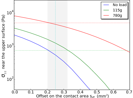
Figure 11: Solid lines: the mean vertical stress as a function of contact area offset. Dotted lines: the applied load, 740 Pa for stage 1, and 5000 Pa for stage 2.

We have tested the mechanical response of our grains by compressing a few individual grains between two steel plates and measuring the force required as a function of the gap between the plates (Fig. 10). The response of the grains is consistent with the Hertz model, and we have extracted from these graphs the value of the grains shear modulus, $850kPa$, which is a reasonable value for a commercial rubber.

The Hertz-Mindlin theory therefore provides us with a suitable model to calculate the contact force from the grain geometry, as long as we have a good estimate of the normal overlap $\xi$ for each contact. Two options can be considered at this stage. i) The normal overlap can be estimated from the distance between grain centres. If the grains are located at positions $\underline{r}_{m}$ and $\underline{r}_{n}$, assuming grains remain spherical, $\xi_{mn}=\frac{1}{2}[R_{m}+R_{n}-|\mathbf{\underline{r}_{m}-\underline{r}_{n}}|]$. The autocorrelation function shows that we expect this quantity to be of the order of a few percent of the grain diameter. Although the grain location is determined accurately, calculation of $\xi$ can be fairly inaccurate due to the anisotropy of the imposed strain causing the grains to deviate significantly from a spherical shape into more ellipsoidal geometries. The centre-centre distance is therefore not a good approach to estimate the contact geometry. ii) Our image processing protocols deliver a sensitive measurement of the contact area (Fig. 4), which provides us with a more reliable way to calculate the forces independently of the centre-centre distances. The contact area $(s_{mn})$, between grains labelled by $m$ and $n$, is related with the normal overlap $\xi_{mn}$ by: $\xi_{mn}=\frac{s_{mn}}{2\pi R}$. This purely local measurement of the force can be applied to any grain geometry, as long as the local curvature of the grain near the contact point can be estimated as well.

2.2.3 Force distribution and stress field

As discussed above, the finite resolution of the CT causes the contact areas to be systematically larger than their real values so this measurement needs to be carefully calibrated. There is de facto a small distance $\delta$, of the order of the voxel size, such that if two surfaces are separated by less than $\delta$, they will appear in contact after segmentation. This results in a systematic enlargement of the contact area, and even detection of false contacts if the separation between grains is less than $\delta$. In the case of spherical elastic grains, the contact area after segmentation would correspond to the geometrical overlap of two grains with each radius being increased by $\delta/2$. Since the contact area is linear with the contact overlap $\xi$, the effect that $\delta$ has on the surface area is equivalent to a systematic offset $s_{off}=\pi R\delta$. However, $\delta$ is a priori unknown and has to be determined by calibrating our measurements.

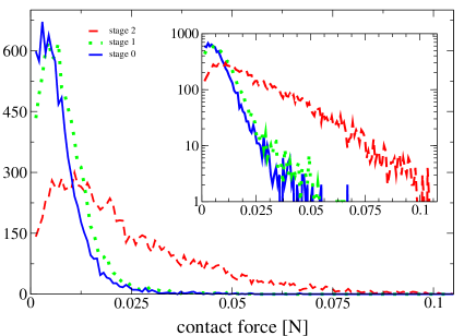
Figure 12: Histograms of normal forces in the sample for all three loading stages.

The mean stress in the vertical direction at the vicinity of the upper interface can be estimated in two independent ways for each loading step; either from the knowledge of the loading mass and geometry of the setup, or by using the contact forces to calculate the stress tensor in the bulk of the pile. We consider a subvolume $\delta v$. Each contact contained in this volume bears a force denoted $\mathbf{\underline{f}_{mn}}$, measured from the contact area $s_{mn}$ between grains indexed by $m$ and $n$. The centre to centre vector is noted $\mathbf{\underline{l}_{m,n}}$. The components of the stress tensor, indexed by $i$ and $j$, are then obtained from the following expression:

$$\sigma_{ij}=\frac{1}{\delta v}\sum_{m,n}\;f^{i}_{mn}l^{j}_{mn}$$ (2)

where the sum is over all contacting pairs of grains in the volume $\delta v$.

In order to measure the offset $\delta$ required to compensate for the segmentation error, we have calculated, using the upper third of the sample, the mean vertical stress $\sigma_{zz}$ we would obtain for a range of values of the surface offset $s_{off}=\pi R\delta$ (Fig. 11). A suitable choice should provide the value of the normal stress consistent with the loading applied on the sample (i.e. where the solid line intersects the dotted line on Fig. 11). Based on this graph, we select $s_{off}\approx$ 0.25 mm², that nearly sets the normal stress to its expected value for the high load value, where the calibration is the most reliable due to the large values of the force and increased number of contacts. This value corresponds, as expected, to the size of a single voxel, confirming the consistency of the method. For stage 0 and 1, however, based on this single threshold calibration, the overall mean stress appears to have been overestimated.

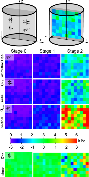
Figure 13: Stress fields in a plane section of the sample for various loads. From top to bottom, i) cartoons showing the location of the section in the sample, along a diameter, and various stress components reported, ii) the stress map in the azimuthal direction $\sigma_{\theta\theta}$, in the radial direction $\sigma_{rr}$, in the vertical direction $\sigma_{zz}$, and shear stress $\sigma_{rz}$.

Once this tool is calibrated, it can be used to probe a number of statistical quantities in the pile. Figure 12 shows the distribution of normal forces in the pile for the three different loads studied here. The 3D bulk measurement of the contact normal forces exhibit a number of features that are characteristic of granular systems. In particular, a salient feature of force measurement presented in this study is that the distributions are primarily exponential for large forces. This is in agreement with earlier measurements in 2D piles Coppersmith:97 ; Liu:95 or at a 3D interface Bruji:05 and also the numerical studies of dynamics of granulated systems Radjai:96 . Another feature often reported in granular dynamics studies OHern:01 ; Majmudar:05 is the presence of a peak or a plateau at low forces. However, this region of the distribution is also where the forces are the most sensitive to image resolution, segmentation and thresholding. We believe a much higher spatial resolution is required before conclusions can be made about the precise shape of the force distribution in the region of low forces, in particular since the mean stress could not be adjusted.

The stress field in the pile is represented by a series of color maps in Fig. 13. These stress maps confirm a number of expected results. In the absence of any loading (stage 0), we observe a slight increase of the stress from top to bottom, in agreement with the fact that only the weight of the grains themselves acts at this stage. The same pattern is observed in all directions. The vertical component of the stress tensor shows an increase with the loading, as well as the radial and azimuthal components. The magnitude of the vertical component is about twice as large as the other two. Another finding of interest concerns the existence of the shear component $(r,z)$. It is also notable that both vertical and radial components of the stress tensor have larger values near the boundary of the confining cylindrical cell at the 2nd stage of compression. Grains at the centre experience a reduced compression, due to their ability to move slightly towards the sides. Lateral grains are however under stronger radial and vertical displacement gradients. These maps are therefore in full agreement with the displacement field measured from the tracking of grains for high loadings (Fig 9).

Conclusion

We have presented in this paper the first measurements of internal stresses in a dry granular system resolved at the single grain scale. We have used here a simple geometry that allows us to calibrate and validate our measurements. In particular, we are now able to quantify, for the same pile, a number of characteristic features. They include mainly the evolution of the coordination number, the 2-point correlation function, the internal displacement fields, force distributions and stress fields, all as a function of loading. Taken together, all these measurements will enable us to better unravel the micromechanical behaviour of granular systems, in particular in quasistatic regimes. It is worth pointing out as well that by measuring the force based on the contact geometry, we are able to deal with non symmetric and polydisperse grains.

Although we have proven that these measurements are realistic and achievable, a number of improvements are still required in order to study more complex cases. We need, in particular, to increase both the spatial statistics (number of grains) and the resolution at the contact scale which will provide a better calibration of the force and therefore a more reliable force measurement in the pile. This will also improve our measurements of coordination number and other geometric quantities. Increased image resolution will also allow the use of stiffer grains which in turn will widen the range of suitable materials to use for the grains. These improvements are achievable in the near future using high resolution nano-focus CT combined with large panel detectors, providing at least a five fold improvement in resolution and speed. The contact model also needs further refinements, so that tangential forces can be estimated from the orientation of the contact zone with respect to the centre-to-centre line. These technical advances, combined with the analysis tools presented here, will contribute to the understanding of a number of open problems. Internal force distribution can now be studied in the bulk, reaching the low force region of the distribution. The mechanics of the material and in particular its mechanical stability rely on the internal organisation of the grain contacts and also the force network. These are quantities that can be directly analysed in 3D, not only statically, but also dynamically by monitoring how an applied load affects each individual grain contact.

The kinematic study of the material can also be qualitatively and quantitatively extended. Not only the local strain can be measured, but the non-affine part of the displacement field is also directly accessible. The latter is increasingly thought to be related with the bulk material properties, in particular when the system is at the onset of rigidity Wyart2008 . How such ideas can apply to 3D frictional granular systems remains to be investigated. In particular, answering such questions will require an extension to our current method so that we can study grain rotation. This would allow us to test the importance of micropolar elasticity in the mechanics of granular systems.

- (1) S.A. Langer, A.J. Liu, Europhysics Letters 49(1), 68 (2000)
- (2) H.P. Zhang, H.A. Makse, Phys. Rev. E 72(1), 011301 (2005). DOI 10.1103/PhysRevE.72.011301
- (3) C.S. O’Hern, S.A. Langer, A.J. Liu, S.R. Nagel, Phys. Rev. Lett. 86(1), 111 (2001). DOI 10.1103/PhysRevLett.86.111
- (4) D. Weaire, J.D. Barry, S. Hutzler, Journal of Physics: Condensed Matter 22(19), 193101 (2010). URL http://stacks.iop.org/0953-8984/22/i=19/a=193101
- (5) F. Radjai, M. Jean, J. Moreau, S. Roux, Phy. Rev. Lett. 77, 274 (1996)
- (6) S.N. Coppersmith, C.h. Liu, S. Majumdar, O. Narayan, T.A. Witten, Phys. Rev. E 53(5), 4673 (1996). DOI 10.1103/PhysRevE.53.4673
- (7) H.A. Makse, D.L. Johnson, L.M. Schwartz, Phys. Rev. Lett. 84(18), 4160 (2000). DOI 10.1103/PhysRevLett.84.4160
- (8) A. Drescher, G. de Josselin de Jong, Journal of the Mechanics and Physics of Solids 20(5), 337 (1972). DOI DOI: 10.1016/0022-5096(72)90029-4. URL http://www.sciencedirect.com/science/article/B6TXB-46J2WW5-D/2/a2dfa0b038f94800648e8202478aa82d
- (9) D. Howell, R.P. Behringer, C. Veje, Phys. Rev. Lett. 82(26), 5241 (1999). DOI 10.1103/PhysRevLett.82.5241
- (10) E. Kolb, J. Cviklinski, J. Lanuza, P. Claudin, E. Clément, Phys. Rev. E 69(3), 031306 (2004). DOI 10.1103/PhysRevE.69.031306
- (11) R. Brockbank, J.M. Huntley, R.C. Ball, Journal de Physique I 7(10), 1521 (1997)
- (12) D.M. Mueth, H.M. Jaeger, S.R. Nagel, Phys. Rev. E 57(3), 3164 (1998). DOI 10.1103/PhysRevE.57.3164
- (13) D.L. Blair, N.W. Mueggenburg, A.H. Marshall, H.M. Jaeger, S.R. Nagel, Phys. Rev. E 63(4), 041304 (2001). DOI 10.1103/PhysRevE.63.041304
- (14) E.I. Corwin, H.M. Jaeger, S.R. Nagel, Nature 435(7045), 1075 (2005)
- (15) G. Lois, J.M. Carlson, Europhysics Letters 80, 5800 (2007). DOI 10.1209/0295-5075/80/58001
- (16) M.D. Mantle, A.J. Sederman, L.F. Gladden, Chemical Engineering Science 56(2), 523 (2001). DOI DOI: 10.1016/S0009-2509(00)00256-6
- (17) A. Kabla, G. Debregeas, J.M. di Meglio, T.J. Senden, Europhysics Letters 71(6), 932 (2005). URL http://stacks.iop.org/0295-5075/71/932
- (18) A.J. Kabla, T.J. Senden, Phys. Rev. Lett. 102(22), 228301 (2009). DOI 10.1103/PhysRevLett.102.228301
- (19) A.J. Dijksman, M. van Hecke, Soft Matter 6(13), 2901 (2010). DOI 10.1039/b925110c. URL http://dx.doi.org/10.1039/b925110c
- (20) J. Brujic, S.F. Edwards, D.V. Grinev, I. Hopkinson, D. Brujic, H.A. Makse, Faraday Discussions 123, 207 (2003). DOI 10.1039/b204414c
- (21) J. Brujić, P. Wang, C. Song, D.L. Johnson, O. Sindt, H.A. Makse, Phys. Rev. Lett. 95(12), 128001 (2005). DOI 10.1103/PhysRevLett.95.128001
- (22) J. Zhou, S. Long, Q. Wang, A.D. Dinsmore, Science 312(5780), 1631 (2006). DOI 10.1126/science.1125151. URL http://www.sciencemag.org/cgi/content/abstract/312/5780/1631
- (23) L.E. Silbert, D. Ertas, G.S. Grest, T.C. Halsey, D. Levine, Phys. Rev. E 65, 031304 (2002)
- (24) T. Aste, M. Saadatfar, T.J. Senden, Phys. Rev. E 71(6), 061302 (2005). DOI 10.1103/PhysRevE.71.061302
- (25) M. Saadatfar, Morphological and mechanical characterisation of microstructured materials. Ph.D. thesis, The Australian National University (2006)
- (26) A. Sakellariou, T.J. Sawkins, T.J. Senden, A. Limaye, Physica A 339, 152 (2004)
- (27) A. Sakellariou, T.J. Senden, T.J. Sawkins, M.A. Knackstedt, M.L. Turner, A.C. Jones, M. Saadatfar, R.J. Roberts, A. Limaye, C.H. Arns, A.P. Sheppard, R.M. Sok, SPIE Annual Meeting 2004 August (2004)
- (28) L.A. Feldkamp, L.C. Davis, J.W. Kress, Journal of Optical Society America A 1, 612 (1984)
- (29) A.P. Sheppard, R.M. Sok, H. Averdunk, Physica A 339, 145 (2004)
- (30) M. Saadatfar, A. Sheppard, M.A. Knackstedt, Advances in X-ray Tomography for Geomaterials ISBN 1-905209-60-6, 269 (2006)
- (31) L. Vincent, P. Soille, IEEE Trans. Pattern Anal. Machine Intell. 13, 583 (1991)
- (32) P. Soille, Morphological Image Analysis: Principles and Applications., vol. ISBN:3540429883 (Springer-Verlag, 2003)
- (33) J.D. Bernal, J. Mason, Nature 188, 910 (1960). DOI doi:10.1038/188910a0
- (34) H.A. Janssen, Zeitschr. d. Vereines deutscher Ingenieure 39(35), 1045 (1895)
- (35) H. Hertz, J. Reine und angewandte Mathematik 92, 156 (1882)
- (36) R. Mindlin, Trans. ASME 71, A (1949)
- (37) K.L. Johnson, Contact mechanics, vol. ISBN-13: 978-0521347969 (Cambridge University Press, 1987)
- (38) S.N. Coppersmith, Physica D: Nonlinear Phenomena 107(2-4), 183 (1997). DOI DOI: 10.1016/S0167-2789(97)00085-7. URL http://www.sciencedirect.com/science/article/B6TVK-3SPGDBV-K/2/21460e860d7f4b5ed6437dee39f8887f. 16th Annual International Conference of the Center for Nonlinear Studies
- (39) C. h. Liu, S.R. Nagel, D.A. Schecter, S.N. Coppersmith, S. Majumdar, O. Narayan, T.A. Witten, Science 269:, 513 (1995). DOI DOI: 10.1126/science.269.5223.513
- (40) S. Majmudar, R.P. Behringer, Nature 435, 1079 (2005). DOI doi:10.1038/nature03805
- (41) M. Wyart, H. Liang, A. Kabla, L. Mahadevan, Phys. Rev. Lett. 101(21), 215501 (2008). DOI 10.1103/PhysRevLett.101.215501