On Approximate electromagnetic cloaking by transformation media

Abstract.

We give a comprehensive study on regularized approximate electromagnetic cloaking via the transformation optics approach. The following aspects are investigated: (i) near-invisibility cloaking of passive media as well as active/radiating sources; (ii) the existence of cloak-busting inclusions without lossy medium lining; (iii) overcoming the cloaking-busts by employing a lossy layer outside the cloaked region; (iv) the frequency dependence of the cloaking performances. We address these issues and connect the obtained asymptotic results to singular ideal cloaking. Numerical verifications and demonstrations are provided to show the sharpness of our analytical study.

Hongyu Liu

Department of Mathematics

University of California, Irvine

Irvine, CA 92697, USA

Email: hongyul1@uci.edu

Ting Zhou

Department of Mathematics

University of Washington

Seattle, WA 98195, USA

Email: tzhou@uw.edu

1. Introduction

A region is said to be cloaked if its contents together with the cloak are invisible to certain noninvasive wave detections. Blueprints for making objects invisible to electromagnetic waves were proposed by Pendry et al. [18] and Leonhardt [11] in 2006. In the case of electrostatics, the same idea was discussed by Greenleaf et al. [8] in 2003. The key ingredient for those constructions is that optical parameters have transformation properties and could be push-forwarded to form new material parameters. The obtained materials/media are called transformation media, which we shall further examine in the current work for cloaking of the full system of Maxwell’s equations.

The transformation-optics-approach-based scheme proposed in [8, 18] is rather singular. This poses much challenge to both theoretical analysis and practical fabrication. In order to avoid the singular structures, several regularized approximate cloaking schemes are proposed in [6, 9, 10, 12, 22]. The works [6] and [22] are based on truncation, whereas in [9, 10, 12], the ‘blow-up-a-point’ transformation in [8, 18] is regularized to be the ‘blow-up-a-small-ball’ transformation. The performances of both regularization schemes have been assessed for cloaking of acoustic waves to give successful near-invisibility effects. Particularly, in [9], the authors show that in order to ‘nearly-cloak’ an arbitrary content, it is necessary to employ an absorbing (‘lossy’) layer lining right outside the cloaked region. Since otherwise, there exist cloaking-busting inclusions which defy any attempts of cloaking. This idea of introducing a lossy layer has recently been intensively investigated for approximate acoustic cloaking (see [15, 16]), whose behaviors are now much well understood. However, very little progress has been made in the study of approximate EM cloaking for full Maxwell’s equations due to the more complicated structure of Maxwell’s equations. This is the main concern of the present article.

We have considered both the ‘truncation-scheme’ and the ‘blow-up-a-small-ball-scheme’ for approximate EM cloaking. However, in our study, the two regularization schemes have the same performances for near-invisibility, so we focus our exposition on the latter one. Based on a model problem, the following aspects on the approximate EM cloaking are addressed in detail.

(i) The near-cloak of EM waves for both passive media and active/radiating sources. For approximate cloaking of passive media, the near-cloak is shown to be within $\rho^{3}$ of the singular ideal cloaking, where $\rho$ is the regularization parameter. Whereas if there is a delta point source present in the cloaked region, the near-cloak is shown to be within $\rho^{2}$ of the perfect cloaking. That is, we could still achieve the near-invisibility effect, but with one order reduction on the approximation. Compared to the near-invisibility assessments in [6, 9, 12, 15, 16, 22] for approximate acoustic cloaking (which is of $\mathcal{O}(\rho)$ when spatial dimension is 3; and $\mathcal{O}(1/\ln\rho)$ when spatial dimension is 2), the performances for near-cloak of EM waves are much better. We point out that the study in [9, 12, 15, 16, 22] lacks the analysis on the approximate cloaking when there is an active/radiating source present inside the cloaked region. Another rather interesting observation we would like to make is that in [5], it is shown one cannot perfectly cloak an $H^{-1}$-source inside the cloaked region since otherwise there would be a conflict with certain ‘hidden’ boundary conditions of the finite energy solutions underlying the singular ideal EM cloaking, but our analysis here shows that one could nearly-cloak a delta point source inside the cloaked region.

(ii) If one allows that the contents in the cloaked region could be arbitrary, then for a fixed near-cloak construction, there always exist cloaking-busting inclusions which defy any attempts of cloaking. These are similar to the resonant inclusions observed in [9] for approximate acoustic cloaking. Following [9], we employ a lossy layer with conducting medium outside the cloaked region to overcome the resonance and re-achieve all the approximate cloaking results for passive media and active sources in (i).

(iii) The performance of the approximate EM cloaking in asymptotically low and high frequency regimes. We show that it is impossible, with a fixed near-cloaking scheme, to obtain cloaking uniformly in frequency, especially for the cloaking of active/radiating objects. Our observation is closely related to the very recent study in [16], where frequency dependence for the approximate acoustic cloaking is considered.

(iv) The limiting behaviors of solutions to regularized approximate cloaking problems, and their connections to finite energy solutions considered in [5] for singular ideal cloaking problems.

Our study has been mainly restricted to spherical cloaking devices with uniform cloaked contents. We base our analysis on spherical wave functions expansions of EM wave fields. Nonetheless, we believe similar results would equally hold for general approximate EM cloaking study.

In this paper, we focus entirely on transformation-optics-approach in constructing cloaking devices. We refer to [4, 17, 23] for state-of-the-art surveys on the rapidly growing literature and many striking applications of transformation optics. But we would also like to mention in passing the other promising cloaking schemes including the one based on anomalous localized resonance [13], and another one based on special (object-dependent) coatings [1].

The rest of the paper is organized as follows. In Section 2, we present the basics on transformation optics in a rather general setting and apply them to the construction of EM cloaking devices. Sections 3–5 are devoted to the main results, respectively on, cloaking of passive media, cloaking of radiating objects and, cloaking-busting inclusions and retaining of cloaking by employing a lossy layer. The numerical experiments are given in Section 6.

2. Transformation optics and electromagnetic cloaking

Let $\Omega$ be a bounded body in $\mathbb{R}^{3}$ whose electric permittivity, conductivity, and magnetic permeability are described by the $\mathbb{R}^{3\times 3}$-valued functions $\varepsilon,\sigma$ and $\mu$, respectively. Consider the time-harmonic electric field $E$ and magnetic field $H$ inside $\Omega$ satisfying Maxwell’s equations

$$\nabla\times E=i\omega\mu H,\quad\nabla\times H=-i\omega(\varepsilon+i\frac{\sigma}{\omega})E+J\qquad\mbox{in\ \ $\Omega$}$$ (2.1)

with $\omega>0$ representing a frequency, $J$ an internal current density. Let $\nu$ be the exterior unit normal on the boundary $\partial\Omega$. By $\Lambda_{\varepsilon,\mu,\sigma,J}^{\omega}$ we denote the linear mapping that takes the tangential component of $E|_{\partial\Omega}$ to that of $H|_{\partial\Omega}$, i.e.,

$$\Lambda_{\varepsilon,\mu,\sigma,J}^{\omega}(\nu\times E|_{\partial\Omega})=\nu\times H|_{\partial\Omega}.$$ (2.2)

$\Lambda_{\varepsilon,\mu,\sigma,J}^{\omega}$ is known as impedance map which encodes the exterior (boundary) measurements of the EM wave fields. In noninvasive detections, one intends to recover the interior object, namely $\mu,\varepsilon,\sigma$ and $J$, by knowing $\Lambda^{\omega}_{\varepsilon,\mu,\sigma,J}$. It is pointed out that knowledge of the impedance map is equivalent to that of the corresponding scattering measurements (cf. [3]). We refer readers to [19] and [20] for uniqueness results of this inverse problem. Throughout the rest of the paper, we shall denote by $\{\Omega;\varepsilon,\mu,\sigma,J\}$ the object (EM medium and internal current) supported in $\Omega$. We would also use $\Lambda_{0}^{\omega}$ to denote the impedance map in the free space; that is, it corresponds to the case with $\varepsilon=\mu=I$, $\sigma=0$ and $J=0$ in $\Omega$. In this context, invisibility cloaking can be generally introduced as follows.

Definition 2.1.

Let $\Omega$ and $D$ be bounded domains in $\mathbb{R}^{3}$ with $D\Subset\Omega$. $\Omega\backslash\bar{D}$ and $D$ represent, respectively, the cloaking region and the cloaked region. $\{\Omega\backslash\bar{D};\varepsilon_{c},\mu_{c},\sigma_{c}\}$ is said to be an invisibility cloaking for the region $D$ if

$$\Lambda_{\varepsilon_{e},\mu_{e},\sigma_{e},J_{e}}^{\omega}=\Lambda_{0}^{\omega}\ \ \ \mbox{on $\partial\Omega$ for all $\omega>0$},$$ (2.3)

where the extended object $\{\Omega;\varepsilon_{e},\mu_{e},\sigma_{e},J_{e}\}$ is given by

$$\{\Omega;\varepsilon_{e},\mu_{e},\sigma_{e},J_{e}\}=\begin{cases}&\{\Omega\backslash\bar{D};\varepsilon_{c},\mu_{c},\sigma_{c},0\}\ \ \mbox{in\ $\Omega\backslash\bar{D}$},\\ &\{D;\varepsilon_{a},\mu_{a},\sigma_{a},J_{a}\}\ \ \ \,\mbox{in\ $D$},\end{cases}$$ (2.4)

with $\{D;\varepsilon_{a},\mu_{a},\sigma_{a},J_{a}\}$ being the target object (which could be arbitrary).

According to Definition 2.1, the cloaking medium $\{\Omega\backslash\bar{D};\varepsilon_{c},\mu_{c},\sigma_{c}\}$ makes the target object, namely the interior EM medium $\{D;\varepsilon_{a},\mu_{a},\sigma_{a}\}$ and the interior source/sink $J$, invisible to exterior boundary measurements.

Next we present the transformation invariance of Maxwell’s equations and transformation properties of EM material parameters, which shall form the key ingredients for our construction of invisibility cloaking devices. To that end, we first briefly discuss the well-posedness of the Maxwell equations (2.1). In the following, let $\Omega$ be an open bounded domain in $\mathbb{R}^{3}$ with smooth boundary. Assume that $\varepsilon,\mu$ and $\sigma$ are in $L^{\infty}(\Omega)^{3\times 3}$, and they have the following properties: There are constants $c_{m},c_{M}>0$ such that for all $x\in\Omega$ and arbitrary $\xi\in\mathbb{R}^{3}$

$$c_{m}|\xi|^{2}\leq\xi^{T}\varepsilon(x)\xi\leq c_{M}|\xi|^{2},\ \ \ c_{m}|\xi|^{2}\leq\xi^{T}\mu(x)\xi\leq c_{M}|\xi|^{2}$$ (2.5)

and

$$0\leq\xi^{T}\sigma\xi\leq c_{M}|\xi|^{2}.$$ (2.6)

We remark that the conditions (2.5) and (2.6) are physical conditions for regular EM media. We also assume that $J\in L^{2}(\Omega)^{3}$. For the Maxwell equations (2.1), we seek solutions $(E,H)\in H(\mbox{curl};\Omega)\times H(\mbox{curl};\Omega)$, where

$$H(\mbox{curl};\Omega)=\{\mathbf{u}\in L^{2}(\Omega)^{3};\nabla\times\mathbf{u}\in L^{2}(\Omega)^{3}\}.$$ (2.7)

We shall not give a complete review on the study of existence and uniqueness of solutions to (2.1) in the setting described above, and we refer to [14] for results related to our present study. It is noted that there is a well-defined continuous impedance map

$$\Lambda_{\varepsilon,\mu,\sigma,J}^{\omega}:\ H^{-1/2}(\mbox{Div};\partial\Omega)\rightarrow H^{-1/2}(\mbox{Div};\partial\Omega),$$ (2.8)

provided $\omega$ avoids a discrete set of frequencies corresponding to resonances (cf. [14]). Here,

$$H^{-\frac{1}{2}}(\mbox{Div};\partial\Omega)=\{\mathbf{s}\in H^{-\frac{1}{2}}(\partial\Omega)^{3};\mathbf{s}\cdot\nu=0\ \mbox{a.e. on $\partial\Omega$}\ \mbox{and}\ \mbox{Div}\,\mathbf{s}\in H^{-\frac{1}{2}}(\partial\Omega)\},$$

with Div denoting the surface divergence on $\partial\Omega$.

Lemma 2.2.

Consider a transformation $\tilde{x}=F(x):\Omega\rightarrow\tilde{\Omega}$, which is assumed to be bi-Lipschitz and orientation-preserving. Let $M=DF:=(\frac{\partial\tilde{x}_{i}}{\partial x_{j}})_{i,j=1}^{3}$ be the Jacobian matrix of $F$. Assume that $(E,H)\in H(\mbox{\emph{curl}};\Omega)\times H(\mbox{\emph{curl}};\Omega)$ are EM fields to (2.1), then for the pull-back fields given by

$$\tilde{E}=(F^{-1})^{*}E:=(M^{T})^{-1}E\circ F^{-1},\ \tilde{H}=(F^{-1})^{*}H:=(M^{T})^{-1}H\circ F^{-1}$$ (2.9)

and

$$\tilde{J}=(F^{-1})^{*}J=\frac{1}{\mbox{\emph{det}}(M)}MJ\circ F^{-1},$$ (2.10)

we have $(\tilde{E},\tilde{H})\in H(\mbox{\emph{curl}};\tilde{\Omega})\times H(\mbox{\emph{curl}};\tilde{\Omega})$ satisfying Maxwell’s equations

$$\tilde{\nabla}\times\tilde{E}=i\omega\tilde{\mu}\tilde{H},\ \ \tilde{\nabla}\times\tilde{H}=-i\omega(\tilde{\varepsilon}+i\frac{\tilde{\sigma}}{\omega})\tilde{E}+\tilde{J}\qquad\mbox{in\ \ $\tilde{\Omega}$},$$ (2.11)

where $\tilde{\nabla}\times$ denotes the curl in the $\tilde{x}$-coordinates, and $\tilde{\varepsilon},\tilde{\mu},\tilde{\sigma}$ are the push-forwards of $\varepsilon,\mu,\sigma$ via $F$, defined respectively by

$$\tilde{\varepsilon}=F_{*}\varepsilon:= \frac{1}{\mbox{\emph{det}}(M)}{M\cdot\varepsilon\cdot M^{T}}\circ F^{-1},$$ (2.12)

$$\tilde{\mu}=F_{*}\mu:= \frac{1}{\mbox{\emph{det}}(M)}{M\cdot\mu\cdot M^{T}}\circ F^{-1},$$ (2.13)

$$\tilde{\sigma}=F_{*}\sigma:= \frac{1}{\mbox{\emph{det}}(M)}{M\cdot\sigma\cdot M^{T}}\circ F^{-1}.$$ (2.14)

Proof.

The key ingredient for the proof of the lemma is the following transformation rule on curl operation (see, e.g. [14])

$$\tilde{\nabla}\times\tilde{E}=\frac{1}{\mbox{det}(M)}M(\nabla\times E)\circ F^{-1},\ \ \tilde{\nabla}\times\tilde{H}=\frac{1}{\mbox{det}(M)}M(\nabla\times H)\circ F^{-1}.$$ (2.15)

Using (2.15) along with (2.1), (2.9) and (2.13), we have

$$\begin{split}\tilde{\nabla}\times\tilde{E}=&\frac{1}{\mbox{det}(M)}(\nabla\times E)\circ F^{-1}=\frac{1}{\mbox{det}(M)}M(i\omega\mu H)\circ F^{-1}\\ =&i\omega\frac{1}{\mbox{det}(M)}M\mu M^{T}(M^{-T}H)\circ F^{-1}=i\omega\tilde{\mu}\tilde{H}.\end{split}$$ (2.16)

Similarly, using (2.15), together with (2.1), (2.9), (2.10), (2.12) and (2.14), we have

$$\begin{split}\tilde{\nabla}\times\tilde{H}=&\frac{1}{\mbox{det}(M)}(\nabla\times H)\circ F^{-1}=\frac{1}{\mbox{det}(M)}(-i\omega\varepsilon_{r}E+J)\circ F^{-1}\\ =&-i\omega\frac{1}{\mbox{det}(M)}M\varepsilon_{r}E\circ F^{-1}+\frac{1}{\mbox{det}(M)}MJ\circ F^{-1}\\ =&-i\omega\tilde{\varepsilon}_{r}\tilde{E}+\tilde{J},\end{split}$$ (2.17)

where

$$\varepsilon_{r}=\varepsilon+i\frac{\sigma}{\omega}\quad\mbox{and}\quad\tilde{\varepsilon}_{r}=\tilde{\varepsilon}+i\frac{\tilde{\sigma}}{\omega}.$$

The proof is completed. ∎

Corollary 1.

Assume that $F:\Omega\rightarrow\Omega$ is bi-Lipschitz and orientation-preserving with $F|_{\partial\Omega}=Id$. Using Green’s identity, it is directly verified that

$$\nu\times E=\tilde{\nu}\times\tilde{E},\ \ \nu\times H=\tilde{\nu}\times\tilde{H}\quad\mbox{on \ $\partial\Omega$},$$ (2.18)

which together with Lemma 2.2 yields

$$\Lambda_{\varepsilon,\mu,\sigma,J}^{\omega}=\Lambda_{F_{*}\varepsilon,F_{*}\mu,F_{*}\sigma,(F^{-1})^{*}J}^{\omega}.$$ (2.19)

Lemma 2.2 and Corollary 1 summarize the basics of transformation optics in a rather general setting, which we shall make essential use of in the present paper. In the rest of this section, we give a short discussion on the singular ideal cloaking device construction considered in [5] and [18] using transformation optics, and introduce the notion of approximate cloaking from a regularization viewpoint. In the sequel, let $B_{r}$ denote the ball centered at the origin with radius $r$. Let $M_{1}=B_{2}$, $M_{2}=B_{1}$ and $M$ be the disjoint union $M=M_{1}\cup M_{2}$. Also, let $N_{1}=B_{2}\backslash\overline{B_{1}}$, $N_{2}=B_{1}$ and $N=N_{1}\cup N_{2}$. Moreover, set $\Sigma:=\partial B_{1}$. Consider the map

$$F_{1}:\,M_{1}\backslash\{0\}\,\rightarrow\,N_{1},\;\;\;\;F_{1}(y)=\left(1+\frac{1}{2}|y|\right)\frac{y}{|y|},\;\;\;0<|y|<2$$ (2.20)

which blows up $\{0\}$ to $N_{2}$ while keeps the boundary $\partial M_{1}$ fixed. In [5] and [18], the authors consider the lossless setting, i.e., one always assume that $\sigma=0$. In the cloaking region $N_{1}$, the EM material parameters of the corresponding cloaking medium are given by

$$\tilde{\mu}(x)=\tilde{\varepsilon}(x)=(F_{1})_{*}I:=\left.\displaystyle\frac{(DF_{1})I(DF_{1})^{T}}{\mbox{det}(DF_{1})}\right|_{y=F_{1}^{-1}(x)},\;\;\;\;x\in N_{1}.$$ (2.21)

In the cloaked region $N_{2}=B_{1}$, we consider cloaking an arbitrary but regular EM medium $(\varepsilon_{0},\mu_{0})$, i.e.,

$$\tilde{\mu}(x)=\mu_{0}(x),\;\;\;\tilde{\varepsilon}(x)=\varepsilon_{0}(x)\;\;\;\;\;x\in N_{2},$$ (2.22)

which can be viewed as the push-forwards of $(\mu_{0},\varepsilon_{0})$ in $M_{2}$ by $F_{2}=Id$. We denote the transformation by

$$F=(F_{1},F_{2}):(M_{1}\backslash\{0\},M_{2})\rightarrow(N_{1},N_{2}).$$ (2.23)

By (2.21) together with straightforward calculations, we have in the standard spherical coordinates $x\mapsto(r\cos\phi\cos\theta,r\sin\phi\cos\theta,r\sin\theta)$ that

$$\tilde{\mu}=\tilde{\varepsilon}=2\frac{(r-1)^{2}}{r^{2}}\mathbf{e}_{r}+2\mathbf{e}_{\theta},\quad 1<r<2,$$ (2.24)

where $\mathbf{e}_{r}$ and $\mathbf{e}_{\theta}$ are respectively, the unit projections along radial and angular directions, i.e.,

$$\mathbf{e}_{r}=I-\hat{x}\hat{x}^{T},\quad\mathbf{e}_{\theta}=\hat{x}\hat{x}^{T},\quad\hat{x}=\frac{x}{|x|}.$$

It is readily seen that as one approaches the cloaking interface $\Sigma$ the cloaking medium becomes singular, since $\tilde{\varepsilon}$ and $\tilde{\mu}$ no longer satisfy the condition (2.5). Finite energy solutions to the singular Maxwell’s equations underlying the cloaking are investigated in [5]. It is shown that $\{0\}$ is a removable singular point. Specifically, let $(\tilde{E},\tilde{H})$ be the EM fields corresponding to $\{N;\tilde{\varepsilon},\tilde{\mu}\}$, then $(E^{+},H^{+})=(F_{1})^{*}(\tilde{E},\tilde{H})$ are EM fields in free space on $M_{1}$, which implies by Corollary 1 that

$$\Lambda_{\tilde{\varepsilon},\tilde{\mu}}^{\omega}=\Lambda_{0}^{\omega}.$$

On the other hand, $(E^{-},H^{-})=(F_{2})^{*}(\tilde{E},\tilde{H})$ satisfy the Maxwell equations

$$\begin{cases}&\nabla\times E^{-}=i\omega\mu_{0}H^{-},\quad\nabla\times H^{-}=-i\omega\varepsilon_{0}E^{-}\ \ \mbox{on $M_{2}$}\\ &\nu\times E^{-}=0,\quad\nu\times H^{-}=0\ \ \mbox{on $\partial M_{2}$}.\end{cases}$$ (2.25)

Generically, one would have $E^{-}=H^{-}=0$ for (2.25) due to the homogeneous ‘hidden’ PEC and PMC boundary conditions in (2.25) on $\partial M_{2}$. Also, due to such ‘hidden’ boundary conditions, it is claimed in [5] that one cannot perfectly cloak a generic internal current in the cloaked region $B_{1}$.

As can be seen from (2.24) the cloaking medium for the ideal cloaking is singular, which poses challenges to both mathematical analysis and physical realization. In order to construct practical nonsingular cloaking devices, it is natural to incorporate regularization by considering approximate cloaking, which we shall investigate in the subsequent sections. We conclude this section by introducing the notion of approximate EM cloaking.

Definition 2.3.

Let $\Omega$ and $D$ be bounded domains in $\mathbb{R}^{3}$ with $D\Subset\Omega$, representing respectively the cloaking region and the cloaked region. Let $\rho>0$ denote a parameter and $e(\rho)$ be a positive function such that

$$e(\rho)\rightarrow 0\quad\mbox{as\ $\rho\rightarrow 0^{+}$}.$$

$\{\Omega\backslash\bar{D};\varepsilon_{c}^{\rho},\mu_{c}^{\rho},\sigma_{c}^{\rho}\}$ is said to be an approximate invisibility cloaking for the region $D$ if

$$\|\Lambda_{\varepsilon_{e}^{\rho},\mu_{e}^{\rho},\sigma_{e}^{\rho},J_{e}}^{\omega}-\Lambda_{0}^{\omega}\|=e(\rho)\quad\mbox{as $\rho\rightarrow 0^{+}$},$$ (2.26)

where the extended object $\{\Omega;\varepsilon_{e}^{\rho},\mu_{e}^{\rho},\sigma_{e}^{\rho},J_{e}\}$ is defined similarly to (2.4) by replacing $\varepsilon_{c},\mu_{c},\sigma_{c}$ with $\varepsilon_{c}^{\rho},\mu_{c}^{\rho},\sigma_{c}^{\rho}$.

According to (2.26), with the cloaking device $\{\Omega\backslash\bar{D};\varepsilon_{c}^{\rho},\mu_{c}^{\rho},\sigma_{c}^{\rho}\}$ we shall have the ‘near-invisibility’ cloaking effect. In order for the invisibility cloaking and approximate invisibility cloaking in Definitions 2.1 and 2.3 make the right sense, throughout the rest of the paper, we always assume that there is a well-defined impedance map $\Lambda_{0}^{\omega}$ in the free space; namely, it is assumed that there is no resonance occurring in the free space.

3. Nonsingular approximate cloaking of passive medium

In this section, we consider the approximate EM cloaking for a relatively simpler case by assuming that all the EM media concerned are lossless, i.e. $\sigma=0$, and also there is no source/sink present, i.e. $J=0$.

For approximate acoustic cloaking by regularization, Kohn et al., in [9], proposed blowing up a small ball $B_{\rho}$ to $B_{1}$ using a nonsingular transformation $F_{\rho}$ which degenerates to the singular transformation $F$ in (2.23) as $\rho\rightarrow 0$, while Greenleaf et al., in [6], proposed blowing up $B_{\rho}$ to $B_{R}$ with $R>1$ by the original singular transformation $F$. For the present study on approximate EM cloaking, we shall focus on the ‘blow-up-a-small-ball-to-$B_{1}$’ scheme and evaluate its performance. However, it is remarked that the other regularization scheme has been verified to yield the same performances for approximate EM cloaking.

3.1. Construction of approximate EM cloaking

Let $0<\rho<1$ denote a regularizer and

$$a=\frac{2(1-\rho)}{2-\rho},\;\;\;\;b=\frac{1}{2-\rho}.$$ (3.1)

Consider the nonsingular transformation from $B_{2}$ to $B_{2}$ defined by

$$x:=F_{\rho}(y)=\left\{\begin{array}[]{ll}F_{\rho}^{(1)}(y)=(a+b|y|)\frac{y}{|y|}&\rho<|y|<2,\\ F_{\rho}^{(2)}(y)=\frac{y}{\rho}&|y|\leq\rho.\end{array}\right.$$ (3.2)

Our approximate cloaking device is obtained by the push-forward of a homogeneous medium in $B_{2}\backslash\overline{B_{\rho}}$ by $F_{\rho}^{(1)}$. Suppose we hide a regular but arbitrary uniform EM medium $(\varepsilon_{0},\mu_{0})$ in the cloaked region $B_{1}$. Then the corresponding EM material parameter in $B_{2}$ is

$$(\tilde{\varepsilon}_{\rho}(x),\tilde{\mu}_{\rho}(x))=\left\{\begin{array}[]{ll}((F_{\rho}^{(1)})_{*}I,(F_{\rho}^{(1)})_{*}I)&1<|x|<2,\\ (\varepsilon_{0},\mu_{0})&|x|<1\end{array}\right.$$

which are obviously nonsingular. The EM fields $(\tilde{E}_{\rho},\tilde{H}_{\rho})\in H(\mbox{curl};B_{2})\times H(\mbox{curl};B_{2})$ corresponding to $\{B_{2};\tilde{\varepsilon}_{\rho},\tilde{\mu}_{\rho}\}$ satisfy Maxwell’s equations

$$\left\{\begin{array}[]{l}\nabla\times\tilde{E}_{\rho}=i\omega\tilde{\mu}_{\rho}(x)\tilde{H}_{\rho},\;\;\;\;\nabla\times\tilde{H}_{\rho}=-i\omega\tilde{\varepsilon}_{\rho}(x)\tilde{E}_{\rho}\;\;\;\;\mbox{in }\;B_{2},\\ \nu\times\tilde{E}_{\rho}|_{\partial B_{2}}=f\in H^{-1/2}(\mbox{Div};\partial B_{2}).\end{array}\right.$$ (3.3)

By Lemma 2.2, the pull-back EM fields

$$(E_{\rho},H_{\rho})=((F_{\rho})^{*}\tilde{E}_{\rho},(F_{\rho})^{*}\tilde{H}_{\rho})\in H(\mbox{curl};B_{2})\times H(\mbox{curl};B_{2})$$

satisfy Maxwell’s equations

$$\left\{\begin{array}[]{l}\nabla\times E_{\rho}=i\omega\mu_{\rho}(y)H_{\rho},\;\;\;\;\nabla\times H_{\rho}=-i\omega\varepsilon_{\rho}(y)E_{\rho},\;\;\;\;\mbox{in }B_{2}\backslash\overline{B_{\rho}},\\ \nu\times E_{\rho}|_{\partial B_{2}}=f\in H^{-1/2}(\mbox{Div};\partial B_{2}),\end{array}\right.$$ (3.4)

where

$$(\varepsilon_{\rho}(y),\mu_{\rho}(y))=\left\{\begin{array}[]{ll}(I,I)&\rho<|y|<2,\\ ((F_{\rho}^{(2)})^{*}\varepsilon_{0},(F_{\rho}^{(2)})^{*}\mu_{0})&|y|<\rho.\end{array}\right.$$

By Corollary 1, we see that

$$\Lambda_{\varepsilon_{\rho},\mu_{\rho}}^{\omega}=\Lambda_{\tilde{\varepsilon}_{\rho},\tilde{\mu}_{\rho}}^{\omega}.$$

Hence, the estimate of $\Lambda_{\tilde{\varepsilon}_{\rho},\tilde{\mu}_{\rho}}^{\omega}$ for the approximate EM cloaking is the same to that of $\Lambda_{\varepsilon_{\rho},\mu_{\rho}}^{\omega}$.

3.2. Convergence and hidden boundary conditions

Henceforth, the following notations for EM fields shall be adopted

$$\tilde{E}_{\rho}:=(\tilde{E}_{\rho}^{+},\tilde{E}_{\rho}^{-}),\;\;\;\;\tilde{H}_{\rho}:=(\tilde{H}_{\rho}^{+},\tilde{H}_{\rho}^{-})\;\;\;\mbox{for }\;x\in(B_{2}\backslash\overline{B_{1}},B_{1})$$

and

$$E_{\rho}:=(E_{\rho}^{+},E_{\rho}^{-}),\;\;\;\;H_{\rho}:=(H_{\rho}^{+},H_{\rho}^{-})\;\;\;\mbox{for }\;y\in(B_{2}\backslash\overline{B_{\rho}},B_{\rho}).$$

We also use $\tilde{E},\tilde{H}$ to represent the finite-energy EM fields considered in [5] for singular ideal cloaking which we discussed earlier in Section 2. (3.3) and (3.4) can be reformulated as the following transmission problems

$$\left\{\begin{array}[]{l}\nabla\times\tilde{E}^{+}_{\rho}=i\omega\tilde{\mu}_{\rho}(x)\tilde{H}^{+}_{\rho},\;\;\;\;\nabla\times\tilde{H}^{+}_{\rho}=-i\omega\tilde{\varepsilon}_{\rho}(x)\tilde{E}^{+}_{\rho}\;\;\;\;\mbox{in }\;B_{2}\backslash\overline{B_{1}},\\ \nabla\times\tilde{E}^{-}_{\rho}=i\omega\mu_{0}\tilde{H}^{-}_{\rho},\;\;\;\;\nabla\times\tilde{H}^{-}_{\rho}=-i\omega\varepsilon_{0}\tilde{E}^{-}_{\rho}\;\;\;\;\mbox{in }\;B_{1},\\ \nu\times\tilde{E}^{+}_{\rho}|_{\Sigma^{+}}=\nu\times\tilde{E}^{-}_{\rho}|_{\Sigma^{-}},\;\;\;\;\nu\times\tilde{H}^{+}_{\rho}|_{\Sigma^{+}}=\nu\times\tilde{H}^{-}_{\rho}|_{\Sigma^{-}},\\ \nu\times\tilde{E}^{+}_{\rho}|_{\partial B_{2}}=f.\end{array}\right.$$ (3.5)

and

$$\left\{\begin{array}[]{l}\nabla\times E^{+}_{\rho}=i\omega H^{+}_{\rho},\;\;\;\;\nabla\times H^{+}_{\rho}=-i\omega E^{+}_{\rho}\;\;\;\;\mbox{in }\;B_{2}\backslash\overline{B_{\rho}},\\ \nabla\times E^{-}_{\rho}=i\omega\mu_{\rho}(y)H^{-}_{\rho},\;\;\;\;\nabla\times H^{-}_{\rho}=-i\omega\varepsilon_{\rho}(y)E^{-}_{\rho}\;\;\;\;\mbox{in }\;B_{\rho},\\ \nu\times E^{+}_{\rho}|_{\Sigma_{\rho}^{+}}=\nu\times E^{-}_{\rho}|_{\Sigma_{\rho}^{-}},\;\;\;\;\nu\times H^{+}_{\rho}|_{\Sigma_{\rho}^{+}}=\nu\times H^{-}_{\rho}|_{\Sigma_{\rho}^{-}},\\ \nu\times E^{+}_{\rho}|_{\partial B_{2}}=f.\end{array}\right.$$ (3.6)

where $\Sigma_{\rho}:=\partial B_{\rho}$.

Our arguments rely heavily on expanding the EM fields into series of spherical wave functions. To that end, we introduce for $n\in\mathbb{Z}^{+}$ and $m\in\mathbb{Z}$,

$$M_{n,\zeta}^{m}(x):=\nabla\times\{xj_{n}(\zeta|x|)Y_{n}^{m}(\hat{x})\},\quad N_{n,\zeta}^{m}(x):=\nabla\times\{xh_{n}^{(1)}(\zeta|x|)Y_{n}^{m}(\hat{x})\},$$

where $\zeta\in\mathbb{C}$ is a complex number and $\hat{x}=x/|x|$ for $x\in\mathbb{R}^{3}$. Here, $Y_{n}^{m}(\hat{x})$ are spherical harmonics and, $h_{n}^{(1)}(z):=j_{n}(z)+iy_{n}(z)$ with $j_{n}(z)$ and $y_{n}(z)$, for $z\in\mathbb{C}$, being the spherical Bessel functions of the first and second kind, respectively. The most important property of such functions for our argument are their asymptotical behavior with respect to small variables:

$$j_{n}(z)=\mathcal{O}(|z|^{n}),\quad h_{n}(z)=\mathcal{O}(|z|^{-n-1}),\quad\mbox{for }|z|\ll 1.$$ (3.7)

We refer to [3] and [14] for more properties of the functions introduced here.

The second Maxwell’s equations in (3.5) and the first of (3.6) would give rise to waves for $x\in B_{1}$

$$\left\{\begin{array}[]{l}\displaystyle\tilde{E}^{-}_{\rho}=\varepsilon_{0}^{-1/2}\sum_{n=1}^{\infty}\sum_{m=-n}^{n}\alpha_{n}^{m}M_{n,k\omega}^{m}+\beta_{n}^{m}\nabla\times M_{n,k\omega}^{m},\\ \displaystyle\tilde{H}^{-}_{\rho}=\frac{1}{ik\omega}\mu_{0}^{-1/2}\sum_{n=1}^{\infty}\sum_{m=-n}^{n}k^{2}\omega^{2}\beta_{n}^{m}M_{n,k\omega}^{m}+\alpha_{n}^{m}\nabla\times M_{n,k\omega}^{m},\end{array}\right.$$ (3.8)

and for $y\in B_{2}\backslash\overline{B_{\rho}}$

$$\left\{\begin{array}[]{l}\displaystyle E^{+}_{\rho}=\sum_{n=1}^{\infty}\sum_{m=-n}^{n}c_{n}^{m}N_{n,\omega}^{m}+d_{n}^{m}\nabla\times N_{n,\omega}^{m}+\gamma_{n}^{m}M_{n,\omega}^{m}+\eta_{n}^{m}\nabla\times M_{n,\omega}^{m},\\ \displaystyle H^{+}_{\rho}=\frac{1}{i\omega}\sum_{n=1}^{\infty}\sum_{m=-n}^{n}\omega^{2}d_{n}^{m}N_{n,\omega}^{m}+c_{n}^{m}\nabla\times N_{n,\omega}^{m}+\omega^{2}\eta_{n}^{m}M_{n,\omega}^{m}+\gamma_{n}^{m}\nabla\times M_{n,\omega}^{m},\end{array}\right.$$ (3.9)

where $k=(\mu_{0}\varepsilon_{0})^{1/2}$.

The following lemma characterizes the asymptotic behaviors of the coefficients in the spherical expansions (3.8) and (3.9) as $\rho$ goes to zero.

Lemma 3.1.

Assume $\omega$ is not an eigenvalue of (3.5), namely, the corresponding homogeneous equations have only trivial solutions. Let $(\tilde{E}_{\rho},\tilde{H}_{\rho})$ be the unique solutions to (3.5), whereas $(E_{\rho},H_{\rho})=((F_{\rho})^{*}\tilde{E}_{\rho},(F_{\rho})^{*}\tilde{H}_{\rho})$ be the unique solutions to (3.6). $(\tilde{E}_{\rho}^{-},\tilde{H}_{\rho}^{-})$ and $(E_{\rho}^{+},H_{\rho}^{+})$ are given by (3.8) and (3.9), respectively, whose coefficients are uniquely determined by the boundary data $f$. As $\rho\rightarrow 0^{+}$, we have

$$\gamma_{n}^{m}=\mathcal{O}(1),\;\;\;\eta_{n}^{m}=\mathcal{O}(1);\;\;\;c_{n}^{m}=\mathcal{O}(\rho^{2n+1}),\;\;\;d_{n}^{m}=\mathcal{O}(\rho^{2n+1}),$$ (3.10)

and

$$\alpha_{n}^{m}=\mathcal{O}(\rho^{n+1}),\;\;\;\beta_{n}^{m}=\mathcal{O}(\rho^{n+1}).$$ (3.11)

Proof.

We need to introduce the vector spherical harmonics

$$U_{n}^{m}:={\frac{1}{\sqrt{n(n+1)}}}\mbox{Grad }Y_{n}^{m},\;\;\;\;\;V_{n}^{m}:=\nu\times U_{n}^{m},$$

where Grad denotes the surface gradient. Define

$$\mathcal{H}_{n}(t):=h^{(1)}_{n}(t)+t{h^{(1)}_{n}}^{\prime}(t),\;\;\;\;\;\mathcal{J}_{n}(t):=j_{n}(t)+tj^{\prime}_{n}(t).$$

For $t\ll 1$, one can verify $\mathcal{J}_{n}(t)=\mathcal{O}(t^{n})$ and $\mathcal{H}_{n}(t)=\mathcal{O}(t^{-n-1})$. Then on a sphere $\partial B_{R}$, we have for $0<R<1$,

$$\left\{\begin{array}[]{l}\displaystyle\nu\times\tilde{E}_{\rho}^{-}|_{\partial B_{R}}=\varepsilon_{0}^{-1/2}\sum_{n=1}^{\infty}\sum_{m=-n}^{n}\sqrt{n(n+1)}\Big{(}\alpha_{n}^{m}j_{n}(k\omega R)U_{n}^{m}\\ \hskip 170.71652pt+\beta_{n}^{m}\frac{1}{R}\mathcal{J}_{n}(k\omega R)V_{n}^{m}\Big{)},\\ \displaystyle\nu\times\tilde{H}_{\rho}^{-}|_{\partial B_{R}}=\frac{1}{ik\omega}\mu_{0}^{-1/2}\sum_{n=1}^{\infty}\sum_{m=-n}^{n}{\sqrt{n(n+1)}}\Big{(}\beta_{n}^{m}k^{2}\omega^{2}j_{n}(k\omega R)U_{n}^{m}\\ \hskip 170.71652pt+\alpha_{n}^{m}\frac{1}{R}\mathcal{J}_{n}(k\omega R)V_{n}^{m}\Big{)},\end{array}\right.$$ (3.12)

whereas for $\rho<R<2$,

$$\left\{\begin{array}[]{l}\displaystyle\nu\times E_{\rho}^{+}|_{\partial B_{R}}=\sum_{n=1}^{\infty}\sum_{m=-n}^{n}{\sqrt{n(n+1)}}\Big{(}c_{n}^{m}h_{n}^{(1)}(\omega R)U_{n}^{m}+d_{n}^{m}\frac{1}{R}\mathcal{H}_{n}(\omega R)V_{n}^{m}\\ \hskip 56.9055pt+\gamma_{n}^{m}j_{n}(\omega R)U_{n}^{m}+\eta_{n}^{m}\frac{1}{R}\mathcal{J}_{n}(\omega R)V_{n}^{m}\Big{)},\\ \displaystyle\nu\times H_{\rho}^{+}|_{\partial B_{R}}=\frac{1}{i\omega}\sum_{n=1}^{\infty}\sum_{m=-n}^{n}{\sqrt{n(n+1)}}\Big{(}\omega^{2}d_{n}^{m}h^{(1)}_{n}(\omega R)U_{n}^{m}\\ \hskip 56.9055pt+c_{n}^{m}\frac{1}{R}\mathcal{H}_{n}(\omega R)V_{n}^{m}+\omega^{2}\eta_{n}^{m}j_{n}(\omega R)U_{n}^{m}+\gamma_{n}^{m}\frac{1}{R}\mathcal{J}_{n}(\omega R)V_{n}^{m}\Big{)}.\end{array}\right.$$ (3.13)

Expanding the boundary value on $\partial B_{2}$ in terms of the vector spherical harmonics, we have

$$f=\sum_{n=1}^{\infty}\sum_{m=-n}^{n}{\sqrt{n(n+1)}}(f_{nm}^{(1)}U_{n}^{m}+f_{nm}^{(2)}V_{n}^{m}),$$ (3.14)

the boundary condition $\nu\times E^{+}_{\rho}|_{\partial B_{2}}=f$ implies

$$\mbox{(R-1)}\;\;\left\{\begin{array}[]{l}c_{n}^{m}h_{n}^{(1)}(2\omega)+\gamma_{n}^{m}j_{n}(2\omega)=f_{nm}^{(1)},\\ d_{n}^{m}\mathcal{H}_{n}(2\omega)+\eta_{n}^{m}\mathcal{J}_{n}(2\omega)=2f_{nm}^{(2)}.\end{array}\right.$$

Since $\tilde{E}_{\rho}=(F_{\rho}^{-1})^{*}E_{\rho}$, the transmission condition on the electric field in (3.5) reads

$$\nu\times\tilde{E}^{+}_{\rho}|_{\Sigma^{+}}=\rho(\nu\times E^{+}_{\rho}|_{\Sigma^{+}_{\rho}})=\nu\times\tilde{E}^{-}_{\rho}|_{\Sigma^{-}}.$$

By (3.12) and (3.13), we have

$$\mbox{(R-2)}\;\;\left\{\begin{array}[]{l}\rho c_{n}^{m}h_{n}^{(1)}(\omega\rho)+\rho\gamma_{n}^{m}j_{n}(\omega\rho)=\varepsilon_{0}^{-1/2}\alpha_{n}^{m}j_{n}(k\omega),\\ d_{n}^{m}\mathcal{H}_{n}(\omega\rho)+\eta_{n}^{m}\mathcal{J}_{n}(\omega\rho)=\varepsilon_{0}^{-1/2}\beta_{n}^{m}\mathcal{J}_{n}(k\omega).\end{array}\right.$$

Similarly, the transmission condition on the magnetic field implies

$$\mbox{(R-3)}\;\;\left\{\begin{array}[]{l}kc_{n}^{m}\mathcal{H}_{n}(\omega\rho)+k\gamma_{n}^{m}\mathcal{J}_{n}(\omega\rho)=\mu_{0}^{-1/2}\alpha_{n}^{m}\mathcal{J}_{n}(k\omega),\\ \rho d_{n}^{m}h_{n}^{(1)}(\omega\rho)+\rho\eta_{n}^{m}j_{n}(\omega\rho)=\mu_{0}^{-1/2}k\beta_{n}^{m}j_{n}(k\omega).\end{array}\right.$$

By (R-2) and (R-3), we have

$$c_{n}^{m}=t_{1}\gamma_{n}^{m},\;\;\;\alpha_{n}^{m}=t_{2}\gamma_{n}^{m},\;\;\;d_{n}^{m}=t_{3}\eta_{n}^{m},\;\;\;\beta_{n}^{m}=t_{4}\eta_{n}^{m},$$ (3.15)

where as $\rho\rightarrow 0^{+}$,

$$\begin{array}[]{l}t_{1}:=\displaystyle\frac{\varepsilon_{0}^{-1/2}k\mathcal{J}_{n}(\omega\rho)j_{n}(k\omega)-\mu_{0}^{-1/2}\rho j_{n}(\omega\rho)\mathcal{J}_{n}(k\omega)}{\mu_{0}^{-1/2}\rho h_{n}^{(1)}(\omega\rho)\mathcal{J}_{n}(k\omega)-\varepsilon_{0}^{-1/2}k\mathcal{H}_{n}(\omega\rho)j_{n}(k\omega)}=\mathcal{O}(\rho^{2n+1}),\\ t_{2}:=\displaystyle\frac{k\rho\mathcal{J}_{n}(\omega\rho)h_{n}^{(1)}(\omega\rho)-k\rho j_{n}(\omega\rho)\mathcal{H}_{n}(\omega\rho)}{\mu_{0}^{-1/2}\rho\mathcal{J}_{n}(k\omega)h_{n}^{(1)}(\omega\rho)-\varepsilon_{0}^{-1/2}kj_{n}(k\omega)\mathcal{H}_{n}(\omega\rho)}=\mathcal{O}(\rho^{n+1}),\\ t_{3}:=\displaystyle\frac{\mu_{0}^{-1/2}k\mathcal{J}_{n}(\omega\rho)j_{n}(k\omega)-\varepsilon_{0}^{-1/2}\rho j_{n}(\omega\rho)\mathcal{J}_{n}(k\omega)}{\varepsilon_{0}^{-1/2}\rho h_{n}^{(1)}(\omega\rho)\mathcal{J}_{n}(k\omega)-\mu_{0}^{-1/2}k\mathcal{H}_{n}(\omega\rho)j_{n}(k\omega)}=\mathcal{O}(\rho^{2n+1}),\\ t_{4}:=\displaystyle\frac{\rho\mathcal{J}_{n}(\omega\rho)h_{n}^{(1)}(\omega\rho)-\rho j_{n}(\omega\rho)\mathcal{H}_{n}(\omega\rho)}{\varepsilon_{0}^{-1/2}\rho\mathcal{J}_{n}(k\omega)h_{n}^{(1)}(\omega\rho)-\mu_{0}^{-1/2}kj_{n}(k\omega)\mathcal{H}_{n}(\omega\rho)}=\mathcal{O}(\rho^{n+1})\end{array}$$ (3.16)

By (R-1), we have

$$\gamma_{n}^{m}=\displaystyle\frac{f_{nm}^{(1)}}{t_{1}h_{n}^{(1)}(2\omega)+j_{n}(2\omega)}=\mathcal{O}(1),\;\;\;\;\eta_{n}^{m}=\displaystyle\frac{2f_{nm}^{(2)}}{t_{3}\mathcal{H}_{n}(2\omega)+\mathcal{J}_{n}(2\omega)}=\mathcal{O}(1).$$ (3.17)

By (3.15), these further imply

$$\alpha_{n}^{m}=\mathcal{O}(\rho^{n+1}),\;\;\;\beta_{n}^{m}=\mathcal{O}(\rho^{n+1}),\;\;\;c_{n}^{m}=\mathcal{O}(\rho^{2n+1}),\;\;\;d_{n}^{m}=\mathcal{O}(\rho^{2n+1}).$$

∎

We are in a position to evaluate the approximate EM cloaking. Our observations are summarized in the following.

Proposition 3.2.

For the approximate EM cloaking, if $\omega$ is not an eigenvalue of (3.5), we have

$$\|\Lambda_{\tilde{\varepsilon}_{\rho},\tilde{\mu}_{\rho}}^{\omega}-\Lambda_{0}^{\omega}\|=\mathcal{O}(\rho^{3})\quad\mbox{as\ $\rho\rightarrow 0^{+}$},$$ (3.18)

where $\|\cdot\|$ denotes the operator norm of the impedance map.

Proof.

We write the EM fields $(E,H)$ propagating in the free space as

$$\left\{\begin{array}[]{l}\displaystyle E=\sum_{n=1}^{\infty}\sum_{m=-n}^{n}a_{n}^{m}M_{n,\omega}^{m}+b_{n}^{m}\nabla\times M_{n,\omega}^{m},\\ H=\displaystyle\frac{1}{i\omega}\sum_{n=1}^{\infty}\sum_{m=-n}^{n}\omega^{2}b_{n}^{m}M_{n,\omega}^{m}+a_{n}^{m}\nabla\times M_{n,\omega}^{m}.\end{array}\right.$$ (3.19)

Consider the boundary condition $\nu\times E|_{\partial B_{2}}=f$ satisfied by the $(E,H)$ fields with $f$ given by (3.14). By straightforward calculations, we have

$$a_{n}^{m}=\frac{f_{nm}^{(1)}}{j_{n}(2\omega)},\;\;\;\;\;b_{n}^{m}=\frac{2f_{nm}^{(2)}}{\mathcal{J}_{n}(2\omega)}.$$

Hence, the tangential magnetic field on the boundary is given by

$$\nu\times H|_{\partial B_{2}}=\frac{1}{i\omega}\sum_{n=1}^{\infty}\sum_{m=-n}^{n}{\sqrt{n(n+1)}}\left(b_{n}^{m}\omega^{2}j_{n}(2\omega)U_{n}^{m}+\frac{1}{i\omega}a_{n}^{m}\frac{1}{2}\mathcal{J}_{n}(2\omega)V_{n}^{m}\right).$$ (3.20)

Compared to $\nu\times H^{+}_{\rho}|_{\partial B_{2}}$ from (3.13), one observes that $c_{n}^{m}$, $d_{n}^{m}$, $\gamma_{n}^{m}-a_{n}^{m}$ and $\eta_{n}^{m}-b_{n}^{m}$ approach zero of order $\mathcal{O}(\rho^{2n+1})$, which in turn implies (3.18). ∎

Proposition 3.2 shows that the approximate cloaking scheme constructed in Section 3.1 actually gives the near-invisibility cloaking effect. Next, we consider the limiting state of the approximate cloaking, showing that it converges to the singular ideal cloaking.

Proposition 3.3.

For the approximate EM cloaking, if $\omega$ is not an eigenvalue of (3.5), we have

$$\tilde{E}_{\rho}\rightarrow\tilde{E}\quad\mbox{and}\quad\tilde{H}_{\rho}\rightarrow\tilde{H}\quad\mbox{as\ $\rho\rightarrow 0^{+}$}.$$ (3.21)

Proof.

We first show

$$(E_{\rho}^{+},H_{\rho}^{+})=(F_{\rho}^{(1)})^{*}(\tilde{E}_{\rho}^{+},\tilde{H}_{\rho}^{+})\rightarrow(E,H)\quad\mbox{as\ $\rho\rightarrow 0^{+}$}.$$ (3.22)

It is easily verified that on any compact subset of $B_{2}$ away from the origin, one has that $(E_{\rho}^{+},H_{\rho}^{+})$ converges to $(E,H)$ at the rate $\mathcal{O}(\rho^{3})$. Indeed, we shall show

$$\|E_{\rho}^{+}-E\|_{L^{2}(B_{2}\backslash\overline{B_{\rho}})}+\|H_{\rho}^{+}-H\|_{L^{2}(B_{2}\backslash\overline{B_{\rho}})}=\mathcal{O}(\rho^{3/2}),$$

which implies (3.22). To that end, we note the following identities

$$\left\{\begin{array}[]{l}M_{n,\omega}^{m}(x)=-\sqrt{n(n+1)}j_{n}(\omega|x|)V_{n}^{m}(\hat{x}),\\ N_{n,\omega}^{m}(x)=-\sqrt{n(n+1)}h_{n}^{m}(\omega|x|)V_{n}^{m}(\hat{x}),\\ \nabla\times M_{n,\omega}^{m}(x)=\displaystyle\frac{\sqrt{n(n+1)}}{|x|}\mathcal{J}_{n}(\omega|x|)U_{n}^{m}(\hat{x})+\frac{n(n+1)}{|x|}j_{n}(\omega|x|)Y_{n}^{m}(\hat{x})\hat{x},\\ \nabla\times N_{n,\omega}^{m}(x)=\displaystyle\frac{\sqrt{n(n+1)}}{|x|}\mathcal{H}_{n}(\omega|x|)U_{n}^{m}(\hat{x})+\frac{n(n+1)}{|x|}h_{n}^{(1)}(\omega|x|)Y_{n}^{m}(\hat{x})\hat{x}.\end{array}\right.$$ (3.23)

By (3.9) and (3.19), we have

$$\begin{split}E_{\rho}^{+}-E=\sum_{n=1}^{\infty}\sum_{m=-n}^{n}&-\sqrt{n(n+1)}[(\gamma_{n}^{m}-a_{n}^{m})j_{n}(\omega|x|)+c_{n}^{m}h_{n}^{(1)}(\omega|x|)]V_{n}^{m}(\hat{x})\\ &+\frac{\sqrt{n(n+1)}}{|x|}[(\eta_{n}^{m}-b_{n}^{m})\mathcal{J}_{n}(\omega|x|)+d_{n}^{m}\mathcal{H}_{n}(\omega|x|)]U_{n}^{m}(\hat{x})\\ &+\frac{n(n+1)}{|x|}[(\eta_{n}^{m}-b_{n}^{m})j_{n}(\omega|x|)+d_{n}^{m}h_{n}^{(1)}(\omega|x|)]Y_{n}^{m}(\hat{x})\hat{x}.\end{split}$$

This implies as $\rho\rightarrow 0^{+}$

$$\begin{split}&\int_{B_{2}\backslash\overline{B_{\rho}}}|E^{+}_{\rho}-E|^{2}dx\\ &\hskip 42.67912pt=\sum_{n=1}^{\infty}\sum_{m=-n}^{n}\int_{\rho}^{2}n(n+1)|(\gamma_{n}^{m}-a_{n}^{m})j_{n}(\omega r)+c_{n}^{m}h_{n}^{(1)}(\omega r)|^{2}r^{2}dr\\ &\hskip 91.04872pt+\int_{\rho}^{2}n(n+1)|(\eta_{n}^{m}-b_{n}^{m})\mathcal{J}_{n}(\omega r)+d_{n}^{m}\mathcal{H}_{n}(\omega r)|^{2}dr\\ &\hskip 91.04872pt+\int_{\rho}^{2}n^{2}(n+1)^{2}|(\eta_{n}^{m}-b_{n}^{m})j_{n}(\omega r)+d_{n}^{m}h_{n}^{(1)}(\omega r)|^{2}dr\\ &\hskip 42.67912pt=\sum_{n=1}^{\infty}\sum_{m=-n}^{n}\mathcal{O}(\rho^{2n+1})=\mathcal{O}(\rho^{3})\end{split}$$

by the convergence orders of the coefficients. Similarly, we have

$$\int_{B_{2}\backslash\overline{B_{\rho}}}|H^{+}_{\rho}-H|^{2}dx=\mathcal{O}(\rho^{3}).$$

On the other hand, it is observed from (3.12) that

$$\left\{\begin{array}[]{l}\nu\times\tilde{E}_{\rho}^{-}|_{\Sigma^{-}}=\displaystyle\varepsilon_{0}^{-1/2}\sum_{n=1}^{\infty}\sum_{m=-n}^{n}\sqrt{n(n+1)}\Big{(}\alpha_{n}^{m}j_{n}(k\omega)U_{n}^{m}\\ \hskip 170.71652pt+\beta_{n}^{m}\mathcal{J}_{n}(k\omega)V_{n}^{m}\Big{)},\\ \nu\times\tilde{H}_{\rho}^{-}|_{\Sigma^{-}}=\displaystyle\frac{1}{ik\omega}\mu_{0}^{-1/2}\displaystyle\sum_{n=1}^{\infty}\sum_{m=-n}^{n}\sqrt{n(n+1)}\Big{(}\beta_{n}^{m}k^{2}\omega^{2}j_{n}(k\omega)U_{n}^{m}\\ \hskip 170.71652pt+\alpha_{n}^{m}\mathcal{J}_{n}(k\omega)V_{n}^{m}\Big{)}\end{array}\right.$$ (3.24)

are both of $\mathcal{O}(\rho^{2})$ as $\rho\rightarrow 0^{+}$. Therefore the homogeneous PEC and PMC conditions naturally appears on the interior cloaking interface $\Sigma^{-}$. This is consistent with the interior ‘hidden’ boundary conditions discovered in [5] for singular ideal cloaking (see also (2.25)), which together with (3.22) implies (3.21). ∎

3.3. Cloak-busting inclusions and frequency dependence

In our earlier discussion, we achieved near-invisibility under the condition that there are no resonances occurring. That is, $\omega$ is not an eigenvalue to (3.3), or equivalently, to (3.4). In fact, if $\omega$ is an eigenvalue to (3.4), the small inclusion $(\varepsilon_{\rho},\mu_{\rho})$ in the free space could have a large effect on the boundary measurement. In this resonance case, one may not even has a well-defined boundary operator $\Lambda_{\varepsilon_{\rho},\mu_{\rho}}^{\omega}$. The failure of the near-invisible cloaking due to such “cloak-busting” inclusion is also observed in the study of approximate acoustic cloaking in [9]. In the following, we shall show a similar result that for a fixed approximate EM cloaking scheme, there always exists certain interior content $(\varepsilon_{0},\mu_{0})$ such that resonance occurs at certain frequency $\omega$. We shall be looking for such triples $(\omega,\varepsilon_{0},\mu_{0})$, or equivalently $(\omega,k,\mu_{0})$, dependent on $\rho$, such that (3.5) is ill-posed. It corresponds to choices of $(\omega,k,\mu_{0})$ such that the coefficient matrices of systems (R-1), (R-2) and (R-3) are singular.

We consider two decoupled systems (R-1-1)–(R-2-1)–(R-3-1) and (R-1-2)–(R-2-2)–(R-3-2) corresponding respectively, to the variables $\{c_{n}^{m},\alpha_{n}^{m},\gamma_{n}^{m}\}$ and $\{d_{n}^{m},\beta_{n}^{m},\eta_{n}^{m}\}$. The coefficient matrices are denoted as $A_{n}$ and $B_{n}$ in the following. By elementary linear algebra manipulations, the augmented matrix for $A_{n}$ for the first system reduces to

$$\left(\begin{array}[]{cccc}h_{n}^{(1)}(2\omega)&0&j_{n}(2\omega)&f_{nm}^{(1)}\\ 0&-\varepsilon_{0}^{-1/2}j_{n}(k\omega)&\rho j_{n}(\omega\rho)-\frac{\rho j_{n}(2\omega)h_{n}^{(1)}(\omega\rho)}{h_{n}^{(1)}(2\omega)}&-\frac{f^{(1)}_{nm}\rho h_{n}^{(1)}(\omega\rho)}{h_{n}^{(1)}(2\omega)}\\ 0&0&\tilde{A}_{n}(3,3)&\tilde{A}_{n}(3,4)\end{array}\right)$$

where

$$\begin{split}\tilde{A}_{n}(3,3)=&\frac{\varepsilon_{0}^{1/2}}{h_{n}^{(1)}(2\omega)j_{n}(k\omega)}\left\{\mu_{0}^{1/2}j_{n}(k\omega)[\mathcal{J}_{n}(\omega\rho)h_{n}^{(1)}(2\omega)-\mathcal{H}_{n}(\omega\rho)j_{n}(2\omega)]\right.\\ &\left.-\rho\mu_{0}^{-1/2}\mathcal{J}_{n}(k\omega)[j_{n}(\omega\rho)h_{n}^{(1)}(2\omega)-h_{n}^{(1)}(\omega\rho)j_{n}(2\omega)]\right\},\end{split}$$

and

$$\tilde{A}_{n}(3,4)=\frac{\varepsilon_{0}^{1/2}f^{(1)}_{nm}}{h_{n}^{(1)}(2\omega)j_{n}(k\omega)}\left\{\rho\mu_{0}^{-1/2}h_{n}^{(1)}(\omega\rho)\mathcal{J}_{n}(k\omega)-\mu_{0}^{1/2}\mathcal{H}_{n}(\omega\rho)j_{n}(k\omega)\right\}.$$

For $\mbox{det}(A_{n})=0$, one can choose $(\omega,k,\mu_{0})$ satisfying

$$\mu_{0}\frac{j_{n}(k\omega)}{\mathcal{J}_{n}(k\omega)}=\rho\frac{j_{n}(\omega\rho)h_{n}^{(1)}(2\omega)-h_{n}^{(1)}(\omega\rho)j_{n}(2\omega)}{\mathcal{J}_{n}(\omega\rho)h_{n}^{(1)}(2\omega)-\mathcal{H}_{n}(\omega\rho)j_{n}(2\omega)},$$ (3.25)

It is easily verified that with this choice, if $f_{nm}^{(1)}\neq 0$, then $\tilde{A}_{n}(3,4)\neq 0$, there exists no solution of $(c_{n}^{m},\alpha_{n}^{m},\gamma_{n}^{m})$. The boundary value problem is ill-posed and one does not have a well-defined boundary impedance map. In like manner, one can find $(\omega,k,\varepsilon_{0})$ such that $\mbox{det}(B_{n})=0$.

Next we consider the performances of the approximate cloaking scheme in extreme frequency regimes. That is, we let $\rho$ and $(\varepsilon_{0},\mu_{0})$ be fixed, and evaluate the approximate cloaking effects as $\omega$ approaches zero or infinity, corresponding the low and high frequency regimes. First, we see that

$$\nu\times H_{\rho}^{+}|_{\partial B_{2}}-\nu\times H|_{\partial B_{2}}=\sum_{n=1}^{\infty}\sum_{m=-n}^{n}g_{nm}^{(1)}U_{n}^{m}+g_{nm}^{(2)}V_{n}^{m},$$

where

$$\begin{split}g_{nm}^{(1)}:=&\frac{\omega}{i}\sqrt{n(n+1)}\left(b_{n}^{m}j_{n}(2\omega)-\eta_{n}^{m}j_{n}(2\omega)-d_{n}^{m}h_{n}^{(1)}(2\omega)\right)\\ =&\displaystyle\frac{-2i\sqrt{n(n+1)}\omega^{2}t_{3}b_{n}^{m}W_{n}(2\omega)}{t_{3}\mathcal{H}_{n}(2\omega)+\mathcal{J}_{n}(2\omega)},\\ =&\frac{-2i\sqrt{n(n+1)}\omega^{2}b_{n}^{m}\left[\varepsilon_{0}\mathcal{J}_{n}(\omega\rho)j_{n}(k\omega)-\rho j_{n}(\omega\rho)\mathcal{J}_{n}(k\omega)\right]W_{n}(2\omega)}{\varepsilon_{0}^{1/2}\mbox{det}(B_{n})},\\ g_{nm}^{(2)}:=&\frac{1}{2i\omega}\sqrt{n(n+1)}\left(a_{n}^{m}\mathcal{J}_{n}(2\omega)-\gamma_{n}^{m}\mathcal{J}_{n}(2\omega)-c_{n}^{m}\mathcal{H}_{n}(2\omega)\right)\\ =&\displaystyle\frac{i\sqrt{n(n+1)}t_{1}a_{n}^{m}W_{n}(2\omega)}{t_{1}h_{n}^{(1)}(2\omega)+j_{n}(2\omega)}\\ =&\frac{i\sqrt{n(n+1)}a_{n}^{m}\left[\mu_{0}\mathcal{J}_{n}(\omega\rho)j_{n}(k\omega)-\rho j_{n}(\omega\rho)\mathcal{J}_{n}(k\omega)\right]W_{n}(2\omega)}{\mu_{0}^{1/2}\mbox{det}(A_{n})}\end{split}$$ (3.26)

with $W_{n}(t):=j_{n}(t){h_{n}^{(1)}}^{\prime}(t)-h_{n}^{(1)}(t)j_{n}^{\prime}(t)$.

We shall address the frequency dependence issue by assuming that the inputs are given by the EM plane waves of the form (6.1). The corresponding coefficients $f_{nm}^{(1)}$ and $f^{(2)}_{nm}$ are given by (6.2), while $a_{n}^{m}$ and $b_{n}^{m}$ are given by (6.3). It is readily seen

$$a_{n}^{m}=\mathcal{O}(1),\qquad b_{n}^{m}=\mathcal{O}(\omega^{-1}).$$

For the low frequency regime with $\omega\ll 1$, by (3.26), it is straightforward to show

$$g_{nm}^{(1)}\sim\omega^{n}\rho^{2n+1},\quad g_{nm}^{(2)}\sim\omega^{n-1}\rho^{2n+1},$$

which implies a satisfactory approximate cloaking. Whereas for the high frequency regime with $\omega\gg 1$, we exclude the influence of resonances from our study by considering the case that $|\mbox{det}(A_{n})|$ and $|\mbox{det}(B_{n})|$ are bounded from below by a positive function $C_{nm}(\omega,\rho)$, where the transmission problem (3.5) is well-posed. Then we consider two separate cases:

• When $1\leq\omega\ll\rho^{-1}$, i.e., $\omega\rho\ll 1$, since $j_{n}(t),h_{n}^{(1)}(t)$ oscillate between $-t^{-1}$ and $t^{-1}$, $\mathcal{J}_{n}(t),\mathcal{H}_{n}(t)$ oscillate between $-1$ and $1$, and $W_{n}(t)\sim t^{-2}$ as $t$ increases, we have

  $$|g_{nm}^{(1)}|\lesssim\frac{(\omega\rho)^{n}\omega^{-2}}{C_{nm}(\omega,\rho)},\quad|g_{nm}^{(2)}|\lesssim\frac{(\omega\rho)^{n}\omega^{-3}}{C_{nm}(\omega,\rho)},$$ (3.27)

  where one can show that $C_{nm}(\omega,\rho)\lesssim\omega^{-n-3}\rho^{-n-1}$. Here and in the following, for two expressions $\mathcal{R}_{1}$ and $\mathcal{R}_{2}$, by “$\mathcal{R}_{1}\lesssim\mathcal{R}_{2}$” we mean “$\mathcal{R}_{1}\leq c\mathcal{R}_{2}$” with a constant $c$.

• For even higher frequency $\omega\gg 1$ such that $\omega\rho\gtrsim 1$, we calculate

  $$|g_{nm}^{(1)}|\lesssim\frac{\omega^{-2}}{C_{nm}(\omega,\rho)},\quad|g_{nm}^{(2)}|\lesssim\frac{\omega^{-3}}{C_{nm}(\omega,\rho)}$$ (3.28)

  where $C_{nm}\lesssim\omega^{-2}$.

By (3.27) and (3.28), we cannot conclude whether or not one can achieve the near-invisibility. However, we conducted extensive numerical experiments to see that one has the near-invisibility in these two cases. These suggest that for the cloaking of passive media, excluding the resonance frequencies, one could achieve the near-invisibility for the approximate cloaking scheme of every frequency. This is sharply different from the case of cloaking active/radiating objects which we shall consider in the next section.

So far, we have been concerned with the cloaking device where the cloaked region is $B_{1}$ and the cloaking medium occupies $B_{2}\backslash\bar{B}_{1}$, which we obtain by using the transformation (3.1)–(3.2). It is remarked here that for arbitrary $0<R_{1}<R_{2}<\infty$, one can construct an approximate cloaking device whose cloaked region is $B_{R_{1}}$ and the cloaking layer is $B_{R_{2}}\backslash\bar{B}_{1}$ by implementing the following transformation

$$x:=G_{\rho}(y)=\left\{\begin{array}[]{ll}G_{\rho}^{(1)}(y)=(a+b|y|)\frac{y}{|y|}&\rho<|y|<R_{2},\\ G_{\rho}^{(2)}(y)=\frac{y}{\rho}&|y|\leq\rho,\end{array}\right.$$

where

$$a=\frac{R_{1}-\rho}{R_{2}-\rho}R_{2},\quad b=\frac{R_{2}-R_{1}}{R_{2}-\rho}.$$

It is readily seen that all our earlier results hold for such construction. The remark applies equally to all our subsequent study.

4. Approximate cloaking with an internal electric current at origin

In this section, we consider the approximate EM cloaking scheme constructed in Section 3.1 in the case that we have an internal electric current present in the cloaked region supported at the origin. The corresponding EM fields verify

$$\left\{\begin{array}[]{l}\nabla\times\tilde{E}_{\rho}=i\omega\tilde{\mu}_{\rho}\tilde{H}_{\rho},\;\;\;\;\;\nabla\times\tilde{H}_{\rho}=-i\omega\tilde{\varepsilon}_{\rho}\tilde{E}_{\rho}+\tilde{J},\;\;\;\;\;\mbox{in }\;B_{2}\\ \nu\times\tilde{E}_{\rho}|_{\partial B_{2}}=f,\end{array}\right.$$ (4.1)

where $\tilde{J}$ has the form

$$\tilde{J}=\sum_{|\alpha|<K}(\partial_{x}^{\alpha}\delta_{0}(x))\mathbf{v}_{\alpha},$$ (4.2)

with $\delta_{0}$ denoting the Dirac delta function at origin and $\mathbf{v}_{\alpha}\in\mathbb{C}^{3}$. The pull-back EM fields satisfy

$$\left\{\begin{array}[]{l}\nabla\times E_{\rho}=i\omega\mu_{\rho}H_{\rho},\;\;\;\;\;\nabla\times H_{\rho}=-i\omega\varepsilon_{\rho}E_{\rho}+J,\;\;\;\;\;\mbox{in }\;B_{2},\\ \nu\times E_{\rho}|_{\partial B_{2}}=f,\end{array}\right.$$ (4.3)

where $J=(F_{\rho}^{2})^{*}\tilde{J}$.

The point electric current $\tilde{J}$ would give rise to a radiating field

$$E_{\tilde{J}}=\displaystyle\sum_{n=1}^{K}\sum_{m=-n}^{n}p_{n}^{m}N_{n,k\omega}^{m}+q_{n}^{m}\nabla\times N_{n,k\omega}^{m}.$$ (4.4)

Hence for $x\in B_{1}$

$$\tilde{E}^{-}_{\rho}=\varepsilon_{0}^{-1/2}\sum_{n=1}^{\infty}\sum_{m=-n}^{n}\alpha_{n}^{m}M_{n,k\omega}^{m}+\beta_{n}^{m}\nabla\times M_{n,k\omega}^{m}+p_{n}^{m}N_{n,k\omega}^{m}+q_{n}^{m}\nabla\times N_{n,k\omega}^{m},$$ (4.5)

where $p_{n}^{m}$ and $q_{n}^{m}$ equal zero when $n>K$. Whereas $E_{\rho}^{+}$ and $H_{\rho}^{+}$ are as in (3.9).

Lemma 4.1.

Assume $\omega$ is not an eigenvalue to (4.1). Let $(\tilde{E}_{\rho},\tilde{H}_{\rho})$ be the EM fields to (4.1) with $\tilde{J}$ given by (4.2), and $(E_{\rho},H_{\rho})=((F_{\rho})^{*}\tilde{E}_{\rho},(F_{\rho})^{*}\tilde{H}_{\rho})$ be the EM fields to (4.3). Given $\tilde{E}_{\rho}^{-}$ as in (4.5) and $E_{\rho}^{+}$ as in (3.9), we have as $\rho\rightarrow 0^{+}$,

$$\gamma_{n}^{m}=\mathcal{O}(1),\;\;\;\eta_{n}^{m}=\mathcal{O}(1);\;\;\;c_{n}^{m}=\mathcal{O}(\rho^{n+1}),\;\;\;d_{n}^{m}=\mathcal{O}(\rho^{n+1}),$$ (4.6)

and

$$\alpha_{n}^{m}=\mathcal{O}(1),\;\;\;\beta_{n}^{m}=\mathcal{O}(1).$$ (4.7)

Proof.

The boundary condition on $\partial B_{2}$ implies (R-1). From the standard transmission conditions, we have

$$\mbox{(R-2')}\left\{\begin{array}[]{l}\rho c_{n}^{m}h_{n}^{(1)}(\omega\rho)+\rho\gamma_{n}^{m}j_{n}(\omega\rho)=\varepsilon_{0}^{-1/2}(\alpha_{n}^{m}j_{n}(k\omega)+p_{n}^{m}h_{n}^{(1)}(k\omega)),\\ d_{n}^{m}\mathcal{H}_{n}(\omega\rho)+\eta_{n}^{m}\mathcal{J}_{n}(\omega\rho)=\varepsilon_{0}^{-1/2}(\beta_{n}^{m}\mathcal{J}_{n}(k\omega)+q_{n}^{m}\mathcal{H}_{n}(k\omega)),\end{array}\right.$$

and

$$\mbox{(R-3')}\left\{\begin{array}[]{l}kc_{n}^{m}\mathcal{H}_{n}(\omega\rho)+k\gamma_{n}^{m}\mathcal{J}_{n}(\omega\rho)=\mu_{0}^{-1/2}(\alpha_{n}^{m}\mathcal{J}_{n}(k\omega)+p_{n}^{m}\mathcal{H}_{n}(k\omega)),\\ \rho d_{n}^{m}h_{n}^{(1)}(\omega\rho)+\rho\eta_{n}^{m}j_{n}(\omega\rho)=\mu_{0}^{-1/2}(k\beta_{n}^{m}j_{n}(k\omega)+kq_{n}^{m}h_{n}^{(1)}(k\omega)).\end{array}\right.$$

Solving (R-2’) and (R-3’), we obtain

$$\begin{array}[]{ll}c_{n}^{m}=t_{1}\gamma_{n}^{m}+t_{1}^{\prime}p_{n}^{m},&\alpha_{n}^{m}=t_{2}\gamma_{n}^{m}+t_{2}^{\prime}p_{n}^{m},\\ d_{n}^{m}=t_{3}\eta_{n}^{m}+t_{3}^{\prime}q_{n}^{m},&\beta_{n}^{m}=t_{4}\eta_{n}^{m}+t_{4}^{\prime}q_{n}^{m},\end{array}$$ (4.8)

where $t_{i}$ $(i=1,2,3,4)$ are given by (3.16) and $t^{\prime}_{i}$ $(i=1,2,3,4)$ are given by

$$\begin{array}[]{l}t_{1}^{\prime}=\displaystyle\frac{h^{(1)}_{n}(k\omega)\mathcal{J}_{n}(k\omega)-\mathcal{H}_{n}(k\omega)j_{n}(k\omega)}{\mu_{0}^{-1/2}\rho h_{n}^{(1)}(\omega\rho)\mathcal{J}_{n}(k\omega)-\varepsilon_{0}^{-1/2}k\mathcal{H}_{n}(\omega\rho)j_{n}(k\omega)}=\mathcal{O}(\rho^{n+1}),\\ t_{2}^{\prime}=\displaystyle\frac{\varepsilon_{0}^{-1/2}kh^{(1)}_{n}(k\omega)\mathcal{H}_{n}(\omega\rho)-\mu_{0}^{-1/2}\rho\mathcal{H}_{n}(k\omega)h^{(1)}_{n}(\omega\rho)}{\mu_{0}^{-1/2}\rho h_{n}^{(1)}(\omega\rho)\mathcal{J}_{n}(k\omega)-\varepsilon_{0}^{-1/2}k\mathcal{H}_{n}(\omega\rho)j_{n}(k\omega)}=\mathcal{O}(1),\\ t_{3}^{\prime}:=\displaystyle\frac{\mathcal{J}_{n}(k\omega)h^{(1)}_{n}(k\omega)-\mathcal{H}_{n}(k\omega)j_{n}(k\omega)}{\varepsilon_{0}^{-1/2}\rho h_{n}^{(1)}(\omega\rho)\mathcal{J}_{n}(k\omega)-\mu_{0}^{-1/2}k\mathcal{H}_{n}(\omega\rho)j_{n}(k\omega)}=\mathcal{O}(\rho^{n+1}),\\ t_{4}^{\prime}:=\displaystyle\frac{\mu_{0}^{-1/2}kh^{(1)}_{n}(k\omega)\mathcal{H}_{n}(\omega\rho)-\varepsilon_{0}^{-1/2}\rho\mathcal{H}_{n}(k\omega)h^{(1)}_{n}(\omega\rho)}{\varepsilon_{0}^{-1/2}\rho h_{n}^{(1)}(\omega\rho)\mathcal{J}_{n}(k\omega)-\mu_{0}^{-1/2}k\mathcal{H}_{n}(\omega\rho)j_{n}(k\omega)}=\mathcal{O}(1).\end{array}$$ (4.9)

Plugging into (R-1), we obtain

$$\gamma_{n}^{m}=\displaystyle\frac{f_{nm}^{(1)}-p_{n}^{m}t_{1}^{\prime}h_{n}^{(1)}(2\omega)}{t_{1}h_{n}^{(1)}(2\omega)+j_{n}(2\omega)}=\mathcal{O}(1),\;\;\;\eta_{n}^{m}=\displaystyle\frac{2f_{nm}^{(2)}-t_{3}^{\prime}q_{n}^{m}\mathcal{H}_{n}(2\omega)}{t_{3}\mathcal{H}_{n}(2\omega)+\mathcal{J}_{n}(2\omega)}=\mathcal{O}(1),$$ (4.10)

which together with (4.8) imply (4.6) and (4.7). ∎

Next, we evaluate the performances of the approximate EM cloaking.

Proposition 4.2.

For the approximate EM cloaking with an internal point current (4.2) present in the cloaked region, if $\omega$ is not an eigenvalue to (4.1), we have

$$\|\Lambda_{\tilde{\varepsilon}_{\rho},\tilde{\mu}_{\rho},\tilde{J}}^{\omega}-\Lambda_{0}^{\omega}\|=\mathcal{O}(\rho^{2})\quad\mbox{as\ $\rho\rightarrow 0^{+}$},$$ (4.11)

where $\|\cdot\|$ denotes the operator norm of the impedance map.

Proof.

On the boundary $\partial B_{2}$, using the expression (3.13) for $\nu\times H_{\rho}^{+}|_{\partial B_{2}}$ and (3.20) for $\nu\times H|_{\partial B_{2}}$, together with the asymptotic estimates of the corresponding coefficients in Lemma 4.1, we have (4.11) by straightforward comparisons, since the coefficients $c_{n}^{m}$, $d_{n}^{m}$, $\gamma_{n}^{m}-a_{n}^{m}$ and $\eta_{n}^{m}-b_{n}^{m}$ converge to zero of order $\mathcal{O}(\rho^{n+1})$. ∎

By Proposition 4.2, we see that one still achieves near-invisibility cloaking even though there is a source/sink present in the cloaked region. That is, the approximate cloaking makes both the passive medium and the active point source/sink nearly-invisible. However, we have one order reduction of the convergence rate. This is due to the extra terms

$$\frac{-p_{n}^{m}t_{1}^{\prime}h_{n}^{(1)}(2\omega)}{t_{1}h_{n}^{(1)}(2\omega)-j_{n}(2\omega)},\;\;\frac{-q_{n}^{m}t_{3}^{\prime}\mathcal{H}_{n}(2\omega)}{t_{3}\mathcal{H}_{n}(2\omega)-\mathcal{J}_{n}(2\omega)},\;\;t_{1}^{\prime}p_{n}^{m},\;\;t_{3}^{\prime}q_{n}^{m}\,\sim\rho^{n+1}$$

in $\gamma_{n}^{m}-a_{n}^{m}$, $\eta_{n}^{m}-b_{n}^{m}$, $c_{n}^{m}$ and $d_{n}^{m}$ respectively, compared to the case without the source/sink.

Next, we consider the limiting status of the approximate cloaking in this case when a point source/sink is present. We have

Proposition 4.3.

Assume $\omega$ is not an eigenvalue to (4.1). Let $(\tilde{E}_{\rho},\tilde{H}_{\rho})$ be the EM fields satisfying (4.1) and $(E_{\rho},H_{\rho})=((F_{\rho})^{*}\tilde{E}_{\rho},(F_{\rho})^{*}\tilde{H}_{\rho})$ be the EM fields satisfying (4.3). Then we have as $\rho\rightarrow 0^{+}$,

$$(E_{\rho}^{+},H_{\rho}^{+})\rightarrow(E,H)$$ (4.12)

with $(E,H)$ being the EM fields on $B_{2}$ in the free space. Also

$$(\tilde{E}_{\rho}^{-},\tilde{H}_{\rho}^{-})\rightarrow(\hat{E}^{-},\hat{H}^{-}),$$ (4.13)

where $(\hat{E}^{-},\hat{H}^{-})$ satisfy the Maxwell equations

$$\nabla\times\hat{E}^{-}=i\omega\mu_{0}\hat{H}^{-},\quad\nabla\times\hat{H}^{-}=-i\omega\varepsilon_{0}\hat{E}^{-}+\tilde{J}\quad\mbox{in \ $B_{1}$}$$ (4.14)

with

$$\nu\times\hat{E}^{-}|_{\Sigma^{-}}\neq 0\quad\mbox{and}\quad\nu\times\hat{H}^{-}|_{\Sigma^{-}}\neq 0.$$ (4.15)

Proof.

By a similar argument to the first part of the proof of Proposition 3.3, one can show that on any compact subset of $B_{2}$ away from the origin, $(E_{\rho}^{+},H_{\rho}^{+})\rightarrow(E,H)$ at the rate $\mathcal{O}(\rho^{2})$, and on $B_{2}\backslash\overline{B_{\rho}}$,

$$\|E_{\rho}^{+}-E\|_{L^{2}(B_{2}\backslash\overline{B_{\rho}})}+\|H_{\rho}^{+}-H\|_{L^{2}(B_{2}\backslash\overline{B_{\rho}})}=\mathcal{O}(\rho^{1/2})\quad\mbox{as\ \ $\rho\rightarrow 0^{+}$}.$$

This proves (4.12). Next, we shall show (4.15) which in turn implies (4.13)–(4.14). On the interior cloaking interface $\Sigma^{-}$, the Cauchy data are given by

$$\left\{\begin{array}[]{l}\nu\times\tilde{E}_{\rho}^{-}|_{\Sigma^{-}}=\displaystyle\varepsilon_{0}^{-1/2}\sum_{n=1}^{\infty}\sum_{m=-n}^{n}\sqrt{n(n+1)}\Big{(}(\alpha_{n}^{m}j_{n}(k\omega)+p_{n}^{m}h_{n}^{(1)}(k\omega))U_{n}^{m}\\ \hskip 142.26378pt+(\beta_{n}^{m}\mathcal{J}_{n}(k\omega)+q_{n}^{m}\mathcal{H}_{n}(k\omega))V_{n}^{m}\Big{)},\\ \nu\times\tilde{H}_{\rho}^{-}|_{\Sigma^{-}}=\displaystyle\frac{\mu_{0}^{-1/2}}{ik\omega}\sum_{n=1}^{\infty}\sum_{m=-n}^{n}\sqrt{n(n+1)}\Big{(}(\alpha_{n}^{m}\mathcal{J}_{n}(k\omega)+p_{n}^{m}\mathcal{H}_{n}(k\omega))V_{n}^{m}\\ \hskip 142.26378pt+k^{2}\omega^{2}(\beta_{n}^{m}j_{n}(k\omega)+q_{n}^{m}h_{n}^{(1)}(k\omega))U_{n}^{m}\Big{)}.\end{array}\right.$$ (4.16)

We observe that as $\rho\rightarrow 0^{+}$

$$\begin{split}\alpha_{n}^{m}j_{n}(k\omega)+p_{n}^{m}h_{n}^{(1)}(k\omega)&=t_{2}\gamma_{n}^{m}j_{n}(k\omega)+(t_{2}^{\prime}j_{n}(k\omega)+h_{n}^{(1)}(k\omega))p_{n}^{m}=\mathcal{O}(\rho),\\ \beta_{n}^{m}\mathcal{J}_{n}(k\omega)+q_{n}^{m}\mathcal{H}_{n}(k\omega)&=t_{4}\eta_{n}^{m}\mathcal{J}_{n}(k\omega)+(t_{4}^{\prime}\mathcal{J}_{n}(k\omega)+\mathcal{H}_{n}(k\omega))q_{n}^{m}=\mathcal{O}(1),\end{split}$$ (4.17)

where

$$\begin{split}&t_{2}^{\prime}j_{n}(k\omega)+h_{n}^{(1)}(k\omega)\sim\frac{\rho h_{n}^{(1)}(\omega\rho)[j_{n}(k\omega)\mathcal{H}_{n}(k\omega)-h_{n}^{(1)}(k\omega)\mathcal{J}_{n}(k\omega)]}{\mu_{0}\mathcal{H}_{n}(\omega\rho)j_{n}(k\omega)}=\mathcal{O}(\rho),\\ &t_{4}^{\prime}\mathcal{J}_{n}(k\omega)+\mathcal{H}_{n}(k\omega)\sim\frac{j_{n}(k\omega)\mathcal{H}_{n}(k\omega)-\mathcal{J}_{n}(k\omega)h_{n}^{(1)}(k\omega)}{j_{n}(k\omega)}=\mathcal{O}(1).\end{split}$$

Similarly, we have

$$\begin{split}&\beta_{n}^{m}j_{n}(k\omega)+q_{n}^{m}h_{n}^{(1)}(k\omega)=\mathcal{O}(\rho),\\ &\alpha_{n}^{m}\mathcal{J}_{n}(k\omega)+p_{n}^{m}\mathcal{H}_{n}(k\omega)=\mathcal{O}(1).\end{split}$$ (4.18)

Plugging (4.17) and (4.18) into (4.16), we have (4.15). The proof is completed. ∎

By Proposition 4.3, we see that as $\rho\rightarrow 0^{+}$, the near-cloak converges to the ideal-cloak. Moreover, in the limiting case, the EM fields in the cloaked region are trapped inside and the cloaked region is completely isolated.

Finally, we consider the frequency dependence for the approximate cloaking of active/radiating objects. Again, we address our study by considering the inputs being EM plane waves as in Section 3.3. By straightforward calculations, the coefficients that characterize the difference of the boundary measurements, i.e. $\nu\times H_{\rho}^{+}|_{\partial B_{2}}-\nu\times H|_{\partial B_{2}}$, associated to terms $U_{n}^{m}$ and $V_{n}^{m}$, verify

$$\begin{split}\tilde{g}_{nm}^{(1)}:=&\frac{\omega}{i}\sqrt{n(n+1)}(b_{n}^{m}j_{n}(2\omega)-\eta_{n}^{m}j_{n}(2\omega)-d_{n}^{m}h_{n}^{(1)}(2\omega))\\ =&\frac{-2i\sqrt{n(n+1)}\omega^{2}W_{n}(2\omega)}{\varepsilon_{0}^{1/2}\mbox{det}(B_{n})}\Big{[}b_{n}^{m}\left(\varepsilon_{0}\mathcal{J}_{n}(\omega\rho)j_{n}(k\omega)-\rho j_{n}(\omega\rho)\mathcal{J}_{n}(k\omega)\right)\\ &-\varepsilon_{0}^{1/2}q_{n}^{m}k\omega W_{n}(k\omega)\Big{]},\\ \tilde{g}_{nm}^{(2)}:=&\frac{1}{2i\omega}\sqrt{n(n+1)}(a_{n}^{m}\mathcal{J}_{n}(2\omega)-\gamma_{n}^{m}\mathcal{J}_{n}(2\omega)-c_{n}^{m}\mathcal{H}_{n}(2\omega))\\ =&\frac{i\sqrt{n(n+1)}W_{n}(2\omega)}{\mu_{0}^{1/2}\mbox{det}(A_{n})}\Big{[}a_{n}^{m}\left(\mu_{0}\mathcal{J}_{n}(\omega\rho)j_{n}(k\omega)-\rho j_{n}(\omega\rho)\mathcal{J}_{n}(k\omega)\right)\\ &-\mu_{0}^{1/2}p_{n}^{m}k\omega W_{n}(k\omega)\Big{]}.\end{split}$$ (4.19)

In the low frequency regime with $\omega\ll 1$, by (4.19) we have

$$\tilde{g}_{nm}^{(1)}\sim\omega^{-n}\rho^{n+1},\quad\tilde{g}_{nm}^{(2)}\sim\omega^{-n-2}\rho^{n+1},$$

which implies that one cannot achieve near-invisibility when $\omega\lesssim\rho^{2/3}$. In the high frequency regime with $\omega\gg 1$, by excluding the resonances and using similar arguments to that in Section 3.3, one can show

$$|\tilde{g}_{nm}^{(1)}|\lesssim\frac{\omega^{-1}}{C_{nm}(\omega,\rho)},\quad|\tilde{g}_{nm}^{(2)}|\lesssim\frac{\omega^{-3}}{C_{nm}(\omega,\rho)},$$ (4.20)

where

$$C_{nm}(\omega,\rho)\lesssim\left\{\begin{array}[]{ll}\omega^{-n-3}\rho^{-n-1}&\omega\rho\ll 1,\,\omega\gtrsim 1,\\ \omega^{-2}&\omega\rho\gtrsim 1.\end{array}\right.$$

By (4.20), one cannot conclude whether or not the near-invisibility is achieved. However, in our numerical experiment given in Section 6.3, we have observed the failure of the approximate cloaking in the high frequency regime. Therefore, it can be concluded that for a fixed approximate cloaking scheme with a point source/sink (4.2) present in the cloaked region, in addition to resonances, the near-invisibility cannot be achieved uniformly in frequency.

5. Approximate cloaking with a lossy layer

In our earlier discussion of lossless approximate cloakings, we have seen the failure of the near-invisibility due to resonant inclusions. Following the spirit in [9] by introducing a damping mechanism to overcome resonances in approximate acoustic cloaking, we surround the cloaked region first by an isotropic conducting layer, then another anisotropic nonconducting layer as described as earlier. To be more specific, given a damping parameter $\tau>0$, our new regularized parameter in $B_{2}$ is given by

$$(\tilde{\mu}_{\rho}(x),\tilde{\varepsilon}_{\rho}(x))=\left\{\begin{array}[]{ll}((F_{2\rho})_{*}I,(F_{2\rho})_{*}I)&1<|x|<2,\\ (\mu_{\tau},\varepsilon_{\tau}):=((F_{2\rho})_{*}I,(F_{2\rho})_{*}(1+i\tau))&\frac{1}{2}<|x|<1,\\ (\mu_{0},\varepsilon_{0})&|x|<\frac{1}{2},\end{array}\right.$$ (5.1)

which is the push-forward of

$$(\mu_{\rho}(y),\varepsilon_{\rho}(y))=\left\{\begin{array}[]{ll}(I,I)&2\rho<|y|<2,\\ (I,1+i\tau)&\rho<|y|<2\rho,\\ ((F_{2\rho}^{-1})_{*}\mu_{0},(F_{2\rho}^{-1})_{*}\varepsilon_{0})&|y|<\rho.\end{array}\right.$$ (5.2)

by the transformation

$$x:=F_{2\rho}(y)=\left\{\begin{array}[]{ll}(\frac{1-2\rho}{1-\rho}+\frac{1}{2(1-\rho)}|y|)\frac{y}{|y|}&2\rho<|y|<2,\\ \frac{y}{2\rho}&|y|\leq 2\rho.\end{array}\right.$$

To assess the approximate cloaking in this setting, we consider the transmission problem

$$\left\{\begin{array}[]{l}\nabla\times E_{1}=i\omega H_{1},\;\;\;\;\;\nabla\times H_{1}=-i\omega E_{1},\;\;\;\;\;\mbox{in }\;2\rho<|y|<2,\\ \nabla\times\tilde{E}_{2}=i\omega\mu_{\tau}\tilde{H}_{2},\;\;\;\;\;\nabla\times\tilde{H}_{2}=-i\omega\varepsilon_{\tau}\tilde{E}_{2},\;\;\;\;\;\mbox{in }\;\frac{1}{2}<|x|<1,\\ \nabla\times\tilde{E}_{3}=i\omega\mu_{0}\tilde{H}_{3},\;\;\;\;\;\nabla\times\tilde{H}_{3}=-i\omega\varepsilon_{0}\tilde{E}_{3}+\tilde{J},\;\;\;\;\;\mbox{in }\;|x|<\frac{1}{2},\\ \nu\times E_{1}|_{\partial B_{2}}=f;\\ \nu\times\tilde{E}_{2}|_{\partial B_{1}^{-}}=2\rho(\nu\times E_{1})|_{\partial B_{2\rho}^{+}},\;\;\;\nu\times\tilde{H}_{2}|_{\partial B_{1}^{-}}=2\rho(\nu\times H_{1})|_{\partial B_{2\rho}^{+}};\\ \nu\times\tilde{E}_{3}|_{\partial B_{1/2}^{-}}=\nu\times\tilde{E}_{2}|_{\partial B_{1/2}^{+}},\;\;\;\nu\times\tilde{H}_{3}|_{\partial B_{1/2}^{-}}=\nu\times\tilde{H}_{2}|_{\partial B_{1/2}^{+}}.\end{array}\right.$$ (5.3)

The problem is well-posed on $B_{2}$ since $\varepsilon_{\tau}$ is complex. Actually, we have

$$(\mu_{\tau},\varepsilon_{\tau})=(2\rho,2\rho(1+i\tau)).$$

Set

$$k_{\tau}:=(\mu_{\tau}\varepsilon_{\tau})^{1/2}=\mathcal{O}(\rho)\quad\mbox{as }\;\rho\rightarrow 0^{+}.$$

We can write the spherical wave expansions of the electric fields as follows

$$\left\{\begin{array}[]{l}E_{1}=\displaystyle\sum_{n=1}^{\infty}\sum_{m=-n}^{n}\gamma_{n}^{m}M_{n,\omega}^{m}+\eta_{n}^{m}\nabla\times M_{n,\omega}^{m}+c_{n}^{m}N_{n,\omega}^{m}+d_{n}^{m}\nabla\times N_{n,\omega}^{m},\\ \tilde{E}_{2}=\displaystyle\varepsilon_{\tau}^{-1/2}\sum_{n=1}^{\infty}\sum_{m=-n}^{n}\tilde{\gamma}_{n}^{m}M_{n,k_{\tau}\omega}^{m}+\tilde{\eta}_{n}^{m}\nabla\times M_{n,k_{\tau}\omega}^{m}+\tilde{c}_{n}^{m}N_{n,k_{\tau}\omega}^{m}+\tilde{d}_{n}^{m}\nabla\times N_{n,k_{\tau}\omega}^{m},\\ \tilde{E}_{3}=\varepsilon_{0}^{-1/2}\displaystyle\sum_{n=1}^{\infty}\sum_{m=-n}^{n}\alpha_{n}^{m}M_{n,k\omega}^{m}+\beta_{n}^{m}\nabla\times M_{n,k\omega}^{m}+p_{n}^{m}N_{n,k\omega}^{m}+q_{n}^{m}\nabla\times N_{n,k\omega}^{m}.\end{array}\right.$$ (5.4)

Then we have

Proposition 5.1.

For any $\omega\in\mathbb{R}^{+}$, assume the EM field $(\tilde{E}_{\rho},\tilde{H}_{\rho})$ satisfies

$$\left\{\begin{array}[]{l}\nabla\times\tilde{E}_{\rho}=i\omega\tilde{\mu}_{\rho}\tilde{H}_{\rho},\;\;\;\;\;\nabla\times\tilde{H}_{\rho}=-i\omega\tilde{\varepsilon}_{\rho}\tilde{E}_{\rho}+\tilde{J},\;\;\;\;\;\mbox{in }\;B_{2}\\ \nu\times\tilde{E}_{\rho}|_{\partial B_{2}}=f,\end{array}\right.$$

where $(\tilde{\mu}_{\rho},\tilde{\varepsilon}_{\rho})$ is the lossy medium given by (5.1). Then the pull-back field $(E_{\rho},H_{\rho})$ satisfies

$$\left\{\begin{array}[]{l}\nabla\times E_{\rho}=i\omega\mu_{\rho}H_{\rho},\;\;\;\;\;\nabla\times H_{\rho}=-i\omega\varepsilon_{\rho}E_{\rho}+J,\;\;\;\;\;\mbox{in }\;B_{2},\\ \nu\times E_{\rho}|_{\partial B_{2}}=f\end{array}\right.$$

with $(\mu_{\rho},\varepsilon_{\rho})$ given by (5.2). Therefore, the fields

$$\begin{split}(E_{1},H_{1})&=(E_{\rho}|_{B_{2}\backslash\overline{B_{2\rho}}},H_{\rho}|_{B_{2}\backslash\overline{B_{2\rho}}}),\\ (\tilde{E}_{2},\tilde{H}_{2})&=(\tilde{E}_{\rho}|_{B_{1}\backslash\overline{B_{1/2}}},\tilde{H}_{\rho}|_{B_{1}\backslash\overline{B_{1/2}}}),\\ (\tilde{E}_{3},\tilde{H}_{3})&=(\tilde{E}_{\rho}|_{B_{1/2}},\tilde{H}_{\rho}|_{B_{1/2}})\end{split}$$

satisfy the transmission problem (5.3). Moreover,

1. If $\tilde{J}=0$, then $(E_{1},\tilde{E}_{2},\tilde{E}_{3})$ is given by (5.4) with $p_{n}^{m}=q_{n}^{m}=0$ for all $n$ and $m$, and

   $$\left\{\begin{array}[]{l}\gamma_{n}^{m}=\mathcal{O}(1),\;\;\eta_{n}^{m}=\mathcal{O}(1),\;\;c_{n}^{m}=\mathcal{O}(\rho^{2n+1}),\;\;d_{n}^{m}=\mathcal{O}(\rho^{2n+1});\\ \tilde{c}_{n}^{m}=\mathcal{O}(\rho^{2n+5/2}),\;\;\tilde{d}_{n}^{m}=\mathcal{O}(\rho^{2n+5/2}),\;\;\tilde{\gamma}_{n}^{m}=\mathcal{O}(\rho^{3/2}),\;\;\tilde{\eta}_{n}^{m}=\mathcal{O}(\rho^{3/2});\\ \alpha_{n}^{m}=\mathcal{O}(\rho^{n+1}),\;\;\beta_{n}^{m}=\mathcal{O}(\rho^{n+1}).\end{array}\right.$$ (5.5)

2. If $\tilde{J}\neq 0$ is given by (4.2), then $(E_{1},\tilde{E}_{2},\tilde{E}_{3})$ is given by (5.4) with $p_{n}^{m},q_{n}^{m}\neq 0$ for some $n$ and $m$, and

   $$\left\{\begin{array}[]{l}\gamma_{n}^{m}=\mathcal{O}(1),\;\;\eta_{n}^{m}=\mathcal{O}(1),\;\;c_{n}^{m}=\mathcal{O}(\rho^{n+1}),\;\;d_{n}^{m}=\mathcal{O}(\rho^{n+1});\\ \tilde{c}_{n}^{m}=\mathcal{O}(\rho^{n+3/2}),\;\;\tilde{d}_{n}^{m}=\mathcal{O}(\rho^{n+3/2}),\;\;\tilde{\gamma}_{n}^{m}=\mathcal{O}(\rho^{-n+1/2})\;\;\tilde{\eta}_{n}^{m}=\mathcal{O}(\rho^{-n+1/2});\\ \alpha_{n}^{m}=\mathcal{O}(1),\;\;\beta_{n}^{m}=\mathcal{O}(1).\end{array}\right.$$ (5.6)

Proof.

In the case that no source/sink is present $(\tilde{J}=0)$, the boundary condition and transmission conditions in (5.3) imply (R-1) and the following equations.

$$\mbox{(R-4)}\left\{\begin{array}[]{l}\displaystyle\varepsilon_{\tau}^{-1/2}\left(\tilde{\gamma}_{n}^{m}j_{n}(k_{\tau}\omega)+\tilde{c}_{n}^{m}h_{n}^{(1)}(k_{\tau}\omega)\right)=2\rho\left(\gamma_{n}^{m}j_{n}(2\omega\rho)+c_{n}^{m}h_{n}^{(1)}(2\omega\rho)\right),\\ \varepsilon_{\tau}^{-1/2}\left(\tilde{\eta}_{n}^{m}\mathcal{J}_{n}(k_{\tau}\omega)+\tilde{d}_{n}^{m}\mathcal{H}_{n}(k_{\tau}\omega)\right)=\eta_{n}^{m}\mathcal{J}_{n}(2\omega\rho)+d_{n}^{m}\mathcal{H}_{n}(2\omega\rho).\end{array}\right.$$

$$\mbox{(R-5)}\displaystyle\left\{\begin{array}[]{l}\mu_{\tau}^{-1/2}\left(\tilde{c}_{n}^{m}\mathcal{H}_{n}(k_{\tau}\omega)+\tilde{\gamma}_{n}^{m}\mathcal{J}_{n}(k_{\tau}\omega)\right)=k_{\tau}\left(c_{n}^{m}\mathcal{H}_{n}(2\omega\rho)+\gamma_{n}^{m}\mathcal{J}_{n}(2\omega\rho)\right),\\ \mu_{\tau}^{-1/2}k_{\tau}\left(\tilde{d}_{n}^{m}h_{n}^{(1)}(k_{\tau}\omega)+\tilde{\eta}_{n}^{m}j_{n}(k_{\tau}\omega)\right)=2\rho\left(d_{n}^{m}h_{n}^{(1)}(2\omega\rho)+\eta_{n}^{m}j_{n}(2\omega\rho)\right).\end{array}\right.$$

$$\mbox{(R-6)}\displaystyle\left\{\begin{array}[]{l}\varepsilon_{0}^{-1/2}\alpha_{n}^{m}j_{n}(\frac{k\omega}{2})=\varepsilon_{\tau}^{-1/2}\left(\tilde{\gamma}_{n}^{m}j_{n}(\frac{k_{\tau}\omega}{2})+\tilde{c}_{n}^{m}h_{n}^{(1)}(\frac{k_{\tau}\omega}{2})\right),\\ \varepsilon_{0}^{-1/2}\beta_{n}^{m}\mathcal{J}_{n}(\frac{k\omega}{2})=\varepsilon_{\tau}^{-1/2}\left(\tilde{\eta}_{n}^{m}\mathcal{J}_{n}(\frac{k_{\tau}\omega}{2})+\tilde{d}_{n}^{m}\mathcal{H}_{n}(\frac{k_{\tau}\omega}{2})\right).\end{array}\right.$$

$$\mbox{(R-7)}\displaystyle\left\{\begin{array}[]{l}\mu_{0}^{-1/2}k_{\tau}\alpha_{n}^{m}\mathcal{J}_{n}(\frac{k\omega}{2})=\mu_{\tau}^{-1/2}k\left(\tilde{c}_{n}^{m}\mathcal{H}_{n}(\frac{k_{\tau}\omega}{2})+\tilde{\gamma}_{n}^{m}\mathcal{J}_{n}(\frac{k_{\tau}\omega}{2})\right),\\ \mu_{0}^{-1/2}k\beta_{n}^{m}j_{n}(\frac{k\omega}{2})=k_{\tau}\mu_{\tau}^{-1/2}\left(\tilde{d}_{n}^{m}h_{n}^{(1)}(\frac{k_{\tau}\omega}{2})+\tilde{\eta}_{n}^{m}j_{n}(\frac{k_{\tau}\omega}{2})\right).\end{array}\right.$$

Solving (R-6-1) and (R-7-1), we obtain

$$\tilde{c}_{n}^{m}=l_{1}\alpha_{n}^{m},\;\;\tilde{\gamma}_{n}^{m}=l_{2}\alpha_{n}^{m},$$

where as $\rho\rightarrow 0^{+}$

$$\begin{split}l_{1}&=\displaystyle\frac{\varepsilon_{\tau}^{1/2}\varepsilon_{0}^{-1/2}\left(j_{n}(\frac{k\omega}{2})\mathcal{J}_{n}(\frac{k_{\tau}\omega}{2})-\mu_{\tau}\mu_{0}^{-1}\mathcal{J}_{n}(\frac{k\omega}{2})j_{n}(\frac{k_{\tau}\omega}{2})\right)}{h_{n}^{(1)}(\frac{k_{\tau}\omega}{2})\mathcal{J}_{n}(\frac{k_{\tau}\omega}{2})-\mathcal{H}_{n}(\frac{k_{\tau}\omega}{2})j_{n}(\frac{k_{\tau}\omega}{2})}=\mathcal{O}(\rho^{n+3/2}),\\ l_{2}&=\displaystyle\frac{\varepsilon_{\tau}^{1/2}\varepsilon_{0}^{-1/2}\left(\mu_{\tau}\mu_{0}^{-1}\mathcal{J}_{n}(\frac{k\omega}{2})h^{(1)}_{n}(\frac{k_{\tau}\omega}{2})-j_{n}(\frac{k\omega}{2})\mathcal{H}_{n}(\frac{k_{\tau}\omega}{2})\right)}{h_{n}^{(1)}(\frac{k_{\tau}\omega}{2})\mathcal{J}_{n}(\frac{k_{\tau}\omega}{2})-\mathcal{H}_{n}(\frac{k_{\tau}\omega}{2})j_{n}(\frac{k_{\tau}\omega}{2})}=\mathcal{O}(\rho^{-n+1/2}).\end{split}$$

Plugging the above quantities into (R-4-1) and (R-5-1), we further have

$$\begin{split}\mbox{(R-4-1)}\;\;\;&-r_{1}\alpha_{n}^{m}+2\rho\varepsilon_{\tau}^{1/2}h_{n}^{(1)}(2\omega\rho)c_{n}^{m}=-2\rho\varepsilon_{\tau}^{1/2}j_{n}(2\omega\rho)\gamma_{n}^{m},\\ \mbox{(R-5-1)}\;\;\;&-r_{2}\alpha_{n}^{m}+\mu_{\tau}^{1/2}k_{\tau}\mathcal{H}_{n}(2\omega\rho)c_{n}^{m}=-\mu_{\tau}^{1/2}k_{\tau}\mathcal{J}_{n}(2\omega\rho)\gamma_{n}^{m},\end{split}$$

where

$$\begin{split}r_{1}&=l_{1}h_{n}^{(1)}(k_{\tau}\omega)+l_{2}j_{n}(k_{\tau}\omega)=\mathcal{O}(\rho^{1/2}),\\ r_{2}&=l_{1}\mathcal{H}_{n}(k_{\tau}\omega)+l_{2}\mathcal{J}_{n}(k_{\tau}\omega)=\mathcal{O}(\rho^{1/2}).\end{split}$$

Then

$$c_{n}^{m}=s_{1}\gamma_{n}^{m},\;\;\alpha_{n}^{m}=s_{2}\gamma_{n}^{m}$$

where

$$\begin{split}s_{1}&=\frac{\mu_{\tau}\mathcal{J}_{n}(2\omega\rho)r_{1}-2\rho j_{n}(2\omega\rho)r_{2}}{2\rho h_{n}^{(1)}(2\omega\rho)r_{2}-\mu_{\tau}\mathcal{H}_{n}(2\omega\rho)r_{1}}=\mathcal{O}(\rho^{2n+1}),\\ s_{2}&=\frac{2\rho\mu_{\tau}\varepsilon_{\tau}^{1/2}\left(-j_{n}(2\omega\rho)\mathcal{H}_{n}(2\omega\rho)+\mathcal{J}_{n}(2\omega\rho)h_{n}^{(1)}(2\omega\rho)\right)}{2\rho h_{n}^{(1)}(2\omega\rho)r_{2}-\mu_{\tau}\mathcal{H}_{n}(2\omega\rho)r_{1}}=\mathcal{O}(\rho^{n+1}).\end{split}$$

By (R-1) as $\rho\rightarrow 0^{+}$, we have

$$\gamma_{n}^{m}=\displaystyle\frac{f_{nm}^{(1)}}{s_{1}h_{n}^{(1)}(2\omega)+j_{n}(2\omega)}=\mathcal{O}(1),$$ (5.7)

which in turn implies

$$c_{n}^{m}=\mathcal{O}(\rho^{2n+1}),\;\;\alpha_{n}^{m}=\mathcal{O}(\rho^{n+1}),$$

$$\tilde{c}_{n}^{m}=\mathcal{O}(\rho^{2n+5/2}),\;\;\tilde{\gamma}_{n}^{m}=\mathcal{O}(\rho^{3/2}).$$

Similar calculations suggests the other estimates in (5.5).

Statement (ii) is derived from solving (R-1), (R-4), (R-5) and

$$\mbox{(R-6')}\left\{\begin{array}[]{l}\varepsilon_{0}^{-1/2}\left(j_{n}(\frac{k\omega}{2})\alpha_{n}^{m}+h_{n}^{(1)}(\frac{k\omega}{2})p_{n}^{m}\right)=\varepsilon_{\tau}^{-1/2}\left(\tilde{\gamma}_{n}^{m}j_{n}(\frac{k_{\tau}\omega}{2})+\tilde{c}_{n}^{m}h_{n}^{(1)}(\frac{k_{\tau}\omega}{2})\right),\\ \varepsilon_{0}^{-1/2}\left(\mathcal{J}_{n}(\frac{k\omega}{2})\beta_{n}^{m}+\mathcal{H}_{n}(\frac{k\omega}{2})q_{n}^{m}\right)=\varepsilon_{\tau}^{-1/2}\left(\tilde{\eta}_{n}^{m}\mathcal{J}_{n}(\frac{k_{\tau}\omega}{2})+\tilde{d}_{n}^{m}\mathcal{H}_{n}(\frac{k_{\tau}\omega}{2})\right),\end{array}\right.$$

$$\mbox{(R-7')}\left\{\begin{array}[]{l}\mu_{0}^{-1/2}k_{\tau}\left(\alpha_{n}^{m}\mathcal{J}_{n}(\frac{k\omega}{2})+p_{n}^{m}\mathcal{H}_{n}\left(\frac{k\omega}{2}\right)\right)=\mu_{\tau}^{-1/2}k\left(\tilde{c}_{n}^{m}\mathcal{H}_{n}(\frac{k_{\tau}\omega}{2})+\tilde{\gamma}_{n}^{m}\mathcal{J}_{n}(\frac{k_{\tau}\omega}{2})\right),\\ \mu_{0}^{-1/2}k\left(\beta_{n}^{m}j_{n}(\frac{k\omega}{2})+q_{n}^{m}h_{n}^{(1)}\left(\frac{k\omega}{2}\right)\right)=k_{\tau}\mu_{\tau}^{-1/2}\left(\tilde{d}_{n}^{m}h_{n}^{(1)}(\frac{k_{\tau}\omega}{2})+\tilde{\eta}_{n}^{m}j_{n}(\frac{k_{\tau}\omega}{2})\right).\end{array}\right.$$

∎

Using Proposition 5.1, all our results in Sections 3 and 4 for the lossless approximate EM cloaking can be shown to hold equally for the lossy approximate cloaking scheme (5.1). We remark briefly on this here.

Remark 5.2.

The estimates in (i) of Proposition 5.1 imply that, without an internal source/sink, the EM fields $(\tilde{E}_{3},\tilde{H}_{3})$ in the cloaked region $B_{1/2}$ degenerates in order $\mathcal{O}(\rho^{2})$. Whereas for the EM fields $(\tilde{E}_{2},\tilde{H}_{2})$ in the lossy layer $B_{1}\backslash\overline{B_{1/2}}$, it is easily seen

$$M_{n,k_{\tau}\omega}^{m},\nabla\times M_{n,k_{\tau}\omega}^{m}=\mathcal{O}(\rho^{n}),\;\;\;\;N_{n,k_{\tau}\omega}^{m},\nabla\times N_{n,k_{\tau}\omega}^{m}=\mathcal{O}(\rho^{-n-1}).$$

Then (5.5) and (5.4) imply that $(\tilde{E}_{2},\tilde{H}_{2})$ degenerate in order $\mathcal{O}(\rho^{2})$ as $\rho$ decays. It follows that the vanishing Cauchy data appears on the inner surface $\partial B_{1}^{-}$. Moreover, the boundary operator on $\partial B_{2}$ of the approximate cloaking converges to that of the ideal cloaking in order $\mathcal{O}(\rho^{3})$.

Remark 5.3.

With an internal point source/sink of the form (4.2) present in the cloaked region, the asymptotic estimates of the coefficients for the corresponding EM fields are given in (ii). By straightforward verification, one can show near-invisibility for the lossy approximate cloaking similar to Proposition 4.2 in the lossless case. On the other hand, one can also show that both the EM fields $(\tilde{E}_{2},\tilde{H}_{2})$ and $(\tilde{E}_{3},\tilde{H}_{3})$ are $\mathcal{O}(1)$, and hence they do not degenerate. Moreover, the Cauchy data on the inner surface $\partial B_{1}^{-}$ does not vanish since by (R-4) and (R-5), the terms associated to $V_{n}^{m}$ of $\nu\times\tilde{E}_{2}$ and $\nu\times\tilde{H}_{2}$ are $\mathcal{O}(1)$. These observations suggest that in the limiting case, the lossy approximate cloaking converges to the ideal cloaking, and the cloaked region is completed isolated with the EM fields trapped inside (see Proposition 4.3 for similar observations in the lossless case).

For the frequency dependence of the performances of the lossy approximate cloakings, we also have completely similar results to those in the lossless case, which we would not repeat here ( see our discussion at the end of Sections 3 and 4).

We conclude this section with two more interesting observations. In [9], for the approximate acoustic cloaking by employing a lossy layer, one needs to require that the damping parameter $\tau\sim\rho^{-2}$, which is not necessary for our present approximate EM cloaking. On the other hand, it is shown in [16] that if $\tau$ is allowed to be $\rho$-dependent, one could achieve near-invisibility uniformly in frequency. However, such result does not hold for the approximate EM cloaking.

6. Numerical experiments

In this section, we carry out some numerical experiments based on the discussions and calculations in Sections 3, 4 and 5. First we introduce an electric plane wave of the form

$$E=e^{-i\omega x\cdot d}P$$ (6.1)

with $d=(1,\theta_{d},\phi_{d})\in\mathbb{S}^{2}$, $P\in\mathbb{C}^{3}$ and $d\cdot P=0$. In the free space, the EM fields $(E,H):=(e^{-i\omega x\cdot d}P,-e^{-i\omega x\cdot d}d\times P)$ satisfy Maxwell’s equations

$$\nabla\times E=i\omega H\quad\nabla\times H=-i\omega E.$$

The spherical wave functions expansions of the EM-fields $(E,H)$ are given by

$$\left\{\begin{array}[]{l}E=\displaystyle\sum_{n=1}^{\infty}\sum_{m=-n}^{n}a_{n}^{m}M_{n,\omega}^{m}(x)+b_{n}^{m}\nabla\times M_{n,\omega}^{m}(x),\\ H=\displaystyle\frac{1}{i\omega}\sum_{n=1}^{\infty}\sum_{m=-n}^{n}\omega^{2}b_{n}^{m}M_{n,\omega}^{m}(x)+a_{n}^{m}\nabla\times M_{n,\omega}^{m}(x),\end{array}\right.$$

where

$$a_{n}^{m}=\frac{f_{nm}^{(1)}}{j_{n}(2\omega)},\;\;\;\;\;b_{n}^{m}=\frac{2f_{nm}^{(2)}}{\mathcal{J}_{n}(2\omega)},$$

and

$$\begin{array}[]{l}f_{nm}^{(1)}:=f_{nm}^{(1)}(d,P)=\displaystyle\frac{4\pi}{n(n+1)i^{n}}\overline{M_{n,{\omega}}^{m}(2d)}\cdot P,\\ \color[rgb]{0,0,0}f_{nm}^{(2)}:=f_{nm}^{(2)}(d,P)=\displaystyle\frac{4\pi}{n(n+1)\omega i^{n-1}}\overline{\nabla\times M_{n,{\omega}}^{m}(2d)}\cdot P.\end{array}$$ (6.2)

By (3.23), we have

$$a_{n}^{m}=-\frac{4\pi}{\sqrt{n(n+1)}i^{n}}\overline{V_{n}^{m}(d)}\cdot P,\quad b_{n}^{m}=\frac{4\pi}{\sqrt{n(n+1)}\omega i^{n-1}}\overline{U_{n}^{m}(d)}\cdot P.$$ (6.3)

On the boundary $\partial B_{2}$, one has

$$\left(\hat{x}\times e^{-i\omega x\cdot d}P\right)\big{|}_{\partial B_{2}}=\sum_{n=1}^{\infty}\sum_{m=-n}^{n}\sqrt{n(n+1)}\left(f_{nm}^{(1)}U_{n}^{m}(\hat{x})+f_{nm}^{(2)}V_{n}^{m}(\hat{x})\right).$$ (6.4)

Figure 1 demonstrates an electric field by taking the first 15 modes in the above expansion; that is, $n$ is up to $N=15$. Throughout all our computations, we shall make use of such truncation when a spherical wave function expansion is considered.

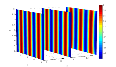
Figure 1. Real part of $E_{1}$, namely the first component of $E$ (sliced at $x=0,1,2$), with the first 15 modes and $\omega=5$, $d=(1,\pi/2,\pi/2)\in\mathbb{S}^{2}$, $P=(1,0,0)^{T}$.

6.1. Lossless approximate cloaking of passive media

Recall in Section 3 that the EM material parameters of our lossless cloaking device are

$$(\tilde{\varepsilon}_{\rho}(x),\tilde{\mu}_{\rho}(x))=\left\{\begin{array}[]{ll}((F_{\rho}^{(1)})_{*}I,(F_{\rho}^{(1)})_{*}I)&1<|x|<2,\\ (\varepsilon_{0},\mu_{0})\mbox{ -- arbitrary constant}&|x|<1.\end{array}\right.$$

Based on the calculations in Lemma 3.1, we depict the EM fields $(\tilde{E}_{\rho},\tilde{H}_{\rho})$ propagating in $\{B_{2};\tilde{\varepsilon}_{\rho},\tilde{\mu}_{\rho}\}$ in Figure 2 with the following boundary condition

$$\hat{x}\times\tilde{E}_{\rho}|_{\partial B_{2}}=\hat{x}\times E,$$ (6.5)

where $E$ is the one demonstrated in Fig 1. It is remarked that the boundary input (6.5) will also be implemented in our subsequent numerical experiments, when a boundary condition is concerned.

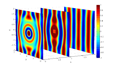
Figure 2. Real part of $({\tilde{E}}_{\rho})_{1}$ (sliced at $x=0,1,2$), with $\omega=5$, $\varepsilon_{0}=\mu_{0}=2$, $\rho=1/6$.

Next, we consider the convergence of the near-cloak to the ideal-cloak. To that end, for the EM fields $(\tilde{E}_{\rho},\tilde{H}_{\rho})$, we compute the deviations of the boundary operators via the formula

$$Er(\rho):=\|\hat{x}\times\tilde{H}_{\rho}-\hat{x}\times H\|_{H^{-\frac{1}{2}}(\mbox{Div};\partial B_{2})}.$$

In our calculations, we shall make use of the following identity from [14],

$$\|\mathbf{\lambda}\|^{2}_{H^{-\frac{1}{2}}(\mbox{Div};\partial B_{2})}=\sum_{n=1}^{\infty}\sum_{m=-n}^{n}\sqrt{n(n+1)}|g^{(1)}_{n,m}|^{2}+\frac{1}{\sqrt{n(n+1)}}|g^{(2)}_{n,m}|^{2},$$

given the vector spherical harmonic expansion of $\mathbf{\lambda}$

$$\mathbf{\lambda}=\sum_{n=1}^{\infty}\sum_{m=-n}^{n}g^{(1)}_{n,m}U_{n}^{m}+g^{(2)}_{n,m}V_{n}^{m}.$$

The convergence rate as $\rho\rightarrow 0^{+}$ is calculated as following

$$r(\rho):=\ln{\frac{Er(\rho_{1})}{Er(\rho_{2})}}\Big{/}\ln{\frac{\rho_{1}}{\rho_{2}}},\quad\rho_{1},\rho_{2}\rightarrow 0^{+}.$$

In Table 1, we list the computational results, which verify Proposition 3.2, i.e., the convergence order is $3$.

$\rho$	$0.1$	$0.05$	$0.01$	$0.005$	$0.002$	$0.001$
$Er(\rho)$	$0.1810$	$0.0139$	$8.42e-05$	$1.02e-06$	$6.42e-07$	$7.97e-08$
$r(\rho)$		$3.703$	$3.173$	$3.044$	$3.020$	$3.009$

Table 1. Convergence rate of boundary operator for the lossless approximate cloaking with $\omega=5$, $\varepsilon_{0}=\mu_{0}=2$.

6.2. Lossless cloaking of active/radiating objects

In this numerical experiment, we study the performance of our lossless approximate cloaking device when an internal point source/sink is present at origin, elaborating to the discussion in Section 4. We apply a delta source $\tilde{J}=\sum_{|\alpha|<K}(\partial_{x}^{\alpha}\delta_{0}(x))\mathbf{v}_{\alpha}$ by introducing a radiating field

$$E_{\tilde{J}}=\displaystyle\sum_{n=1}^{K}\sum_{m=-n}^{n}p_{n}^{m}N_{n,k\omega}^{m}+q_{n}^{m}\nabla\times N_{n,k\omega}^{m},$$

with known $p_{n}^{m}$ and $q_{n}^{m}$, into the electric field $E_{\rho}^{-}$ inside the virtue inclusion $B_{\rho}$. In Figure 3 and Table 2, we choose $p_{1}^{-1}=p_{1}^{0}=p_{1}^{1}=5$, $q_{1}^{-1}=q_{1}^{0}=q_{1}^{1}=2$ and $q_{n}^{m}=p_{n}^{m}=0$ otherwise. From Figure 3, we see that one could still achieve near-invisibility, and the EM fields in the cloaked region is almost trapped inside. Table 2 verifies that the convergence order of the near-cloak is 2, which is consistent with Proposition 4.2.

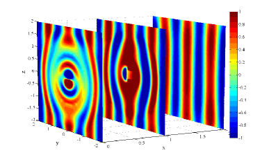
Figure 3. Real part of $({\tilde{E}}_{\rho})_{1}$ for the cloaking problem (sliced at $x=0,1,2$) with a delta source at the origin, $\omega=5$, $\varepsilon_{0}=\mu_{0}=2$, $\rho=1/12$.

$\rho$	$0.1$	$0.05$	$0.01$	$0.005$	$0.002$	$0.001$
$Er(\rho)$	$1.9787$	$0.3509$	$0.0114$	$0.0028$	$4.41e-04$	$1.10e-04$
$r(\rho)$		$2.495$	$2.129$	$2.031$	$2.013$	$2.006$

Table 2. Convergence rate of boundary operator for the lossless approximate cloaking with a delta source, $\omega=5$, $\varepsilon_{0}=\mu_{0}=2$.

6.3. Cloak-busting inclusions and frequency dependence

In Section 3.3, we have shown the failure of lossless cloaking due to resonances. In Figures 4, for a fixed $\rho$, the first mode ($n=1$) of boundary errors $Er(\rho)$ are plotted vs frequency $\omega$, for both passive and active cloaking. We observe blowups of the errors at resonant frequencies, where the determinants $\mbox{det}(A_{n})$ and $\mbox{det}(B_{n})$ ($n=1$) vanish (see Figure 5 for those resonance frequencies).

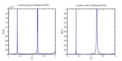
Figure 4. Boundary error for mode $n=1$. Left: lossless cloaking (no source). Right: lossless cloaking (with a source). $\rho=0.01$, $\omega\in[1,3]$.

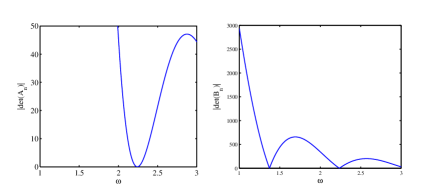
Figure 5. Frequency dependence of determinants of coefficients system (R-1), (R-2) and (R-3). $\rho=0.01$, $\omega\in[1,3]$.

In fact, we have numerically shown that for every frequency $\omega$ and $\rho$, there is a choice of ‘cloaking-busting’ inclusion in $B_{1}$, e.g., a pair of parameters $(\varepsilon_{0},\mu_{0})$ satisfying (3.25), such that the lossless construction is resonant. In Figure 6, an example of such resonant inclusion at mode $n=1$ is plotted against $\rho$ for a fixed frequency. One can see that as $\rho\rightarrow 0^{+}$, the EM parameters of the inclusion become singular, namely, $\varepsilon_{0}\rightarrow\infty$ and $\mu_{0}\rightarrow 0$.

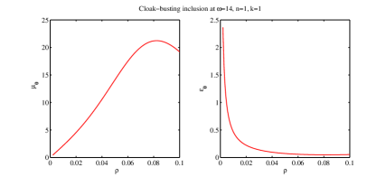
Figure 6. EM parameters $(\mu_{0},\varepsilon_{0})$ for a cloak-busting inclusion at $n=1$ $\omega=14$ with $k=1$.

As discussed in Section 3.3 and Section 5, Figure 7 demonstrates that both the lossless (excluding the resonant frequencies) and lossy cloaking schemes work well in the low frequency regime, namely when $\omega\ll 1$, without any source/sink present in the cloaked region. In Sections 4 and 5, when a point source/sink is present at the origin, we see that both the lossless and lossy cloaking schemes fail when $\omega\lesssim\rho^{2/3}$, as shown in Figure 8. For higher frequencies, the behaviors of the cloaking schemes are not deterministic. Nonetheless, we show in Figure 9 that the lossless cloaking of active/radiating objects (excluding resonant frequencies) generates relatively large boundary error $Er(\rho)$ when $\omega\gg 1$.

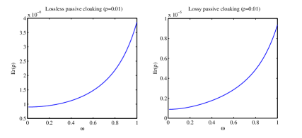
Figure 7. Approximate cloaking performance in low frequency regime $\omega\in[0,1]$. Left: boundary error ($n=1$) for lossless cloaking (no source). Right: boundary error ($n=1$) for lossy cloaking (no source). $\rho=0.01$.

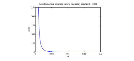
Figure 8. Boundary error ($n=1$) for cloaking with a source. Approximate cloaking compromises in low frequency regime. $\rho=0.01$.

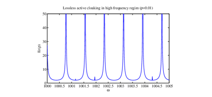
Figure 9. Approximate cloaking (with a source) performance in high frequency regime . Boundary error ($n=1$) $Er(\rho)>2$ for $\omega\in[1000,1005]$. $\rho=0.01$.

6.4. Lossy approximate cloaking

According to our discussion in Section 5, we employ a lossy layer right between the cloaking layer and the cloaked region. In Figure 10, we show how the EM-fields propagate in such a lossy construction of approximate cloaking. One can see that near-invisibility is achieved. In Table 3, the convergence order of the lossy near-cloak of passive media as $\rho\rightarrow 0^{+}$ is shown to be 3, which is consistent with Remark 5.2. It is recalled that for the lossy approximate cloaking, the EM parameters in $B_{2}$ are given by

$$(\tilde{\mu}_{\rho}(x),\tilde{\varepsilon}_{\rho}(x))=\left\{\begin{array}[]{ll}((F_{2\rho})_{*}I,(F_{2\rho})_{*}I)&1<|x|<2,\\ (\mu_{\tau},\varepsilon_{\tau}):=((F_{2\rho})_{*}I,(F_{2\rho})_{*}(1+i\tau)I)&\frac{1}{2}<|x|<1,\\ (\mu_{0},\varepsilon_{0})&|x|<\frac{1}{2}.\end{array}\right.$$

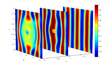
Figure 10. Real part of $({\tilde{E}}_{\rho})_{1}$ for the lossy approximate cloaking problem (sliced at $x=0,1,2$), with $\omega=5$, $\varepsilon_{0}=\mu_{0}=2$, $\rho=1/6$.

$\rho$	$0.1$	$0.05$	$0.01$	$0.005$	$0.002$	$0.001$
$Er(\rho)$	$0.2733$	$0.0455$	$3.75e-04$	$4.69e-05$	$3.00e-06$	$3.75e-07$
$r(\rho)$		$2.5867$	$2.9818$	$2.9998$	$2.9998$	$2.9998$

Table 3. Convergence rate of boundary operator for lossy approximate cloaking of passive medium, with frequency $\omega=5$, $\varepsilon_{0}=\mu_{0}=2$, damping parameter $\tau=3$.

At last, we demonstrate the frequency dependence of our lossy approximate cloaking scheme in Figure 11 without a source/sink. Observe that the resonant frequencies disappear. However, we observe some frequencies at which the boundary error $Er(\rho)$ is relatively large. We believe such frequencies are those very close to the poles or transmission eigenvalues in the complex plane of the boundary value problem. It is remarked that such phenomenon could also be observed in the lossless approximate cloaking. If there is a point source present at the origin, we would have the similar numerical result as the case considered in Figure 9 for the lossless cloaking.

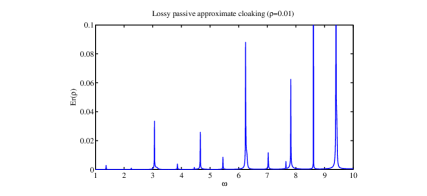
Figure 11. Boundary error ($n=1$) of lossy approximate cloaking (no source). $\rho=0.01$.

References

• [1] Alu, A. and Engheta, N., Achieving transparency with plasmonic and metamaterial coatings, Phys. Rev. E 72 (2005), 016623.
• [2] Calderón, A. P., On an inverse boundary value problem, Seminar on Numerical Analysis and its Applications to Continuum Physics (Río de Janeiro, 1980), pp. 65–73, Soc. Brasil. Mat., Río de Janeiro, 1980.
• [3] Colton, D. and Kress, R., “Inverse acoustic and electromagnetic scattering theory,” 2nd edition Springer-Verlag, New York, 1998.
• [4] Greenleaf, A., Kurylev, Y., Lassas, M., and Uhlmann, G., Cloaking devices, electromagnetic wormholes and transformation optics, SIAM Review, 51 (2009), 3–33.
• [5] Greenleaf, A., Kurylev, Y., Lassas, M. and Uhlmann, G., Full-wave invisibility of active devices at all frequencies, Commu. Math. Phys., 275 (2007), 749–789.
• [6] Greenleaf, A., Kurylev, Y., Lassas, M. and Uhlmann, G., Isotropic transformation optics: approximate acoustic and quantum cloaking, New J. Phys., 10 (2008), 115024.
• [7] Greenleaf, A., Kurylev, Y., Lassas, M. and Uhlmann, G., Improvement of cylindrical cloaking with the SHS lining, Opt. Express, 15 (2007), 12717–12734.
• [8] Greenleaf, A., Lassas, M. and Uhlmann, G., On nonuniqueness for Calderón’s inverse problem, Math. Res. Lett., 10 (2003), 685.
• [9] Kohn, R. V., Onofrei, D., Vogelius, M. S. and Weinstein, M. I., Cloaking via change of variables for the Helmholtz equation, Comm. Pure Appl. Math., 63 (2010), 0973–1016..
• [10] Kohn, R. V., Shen, H., Vogelius, M. S. and Weinstein, M. I., Cloaking via change of variables in electric impedance tomography, Inverse Problems, 24 (2008), 015016.
• [11] Leonhardt, U., Optical conformal mapping, Science, 312 (2006), 1777–1780.
• [12] Liu, H. Y., Virtual reshaping and invisibility in obstacle scattering, Inverse Problems, 25 (2009), 045006.
• [13] Milton, G. W. and Nicorovici, N.-A. P., On the cloaking effects associated with anomalous localized resonance, Proc. Roy. Soc. A, 462 (2006), 3027–3095.
• [14] Monk, P., Finite Element Methods for Maxwell’s Equations, Oxford University Press, New York, 2003.
• [15] Nguyen, H. M., Cloaking via change of variables for the Helmholtz equation in the whole space, Commu. Pure Appl. Math., to appear.
• [16] Nguyen, H. M. and Vogelius, M., Full range scattering estimates and their application cloaking, preprint, 2010
• [17] Norris, A. N., Acoustic cloaking theory, Proc. R. Soc. A, 464 (2008), 2411-2434.
• [18] Pendry, J. B., Schurig, D., and Smith, D. R., Controlling Electromagnetic Fields, Science, 312 (2006), 1780–1782.
• [19] Ola, P., Päivärinta, L. and Somersalo, E., An inverse boundary value problem in electrodynamics, Duke Math. J., 70 (1993), no. 3, 617–653.
• [20] Ola, P. and Somersalo, E., Electromagnetic inverse problems and generalized Sommerfeld potentials, SIAM J. Appl. Math., 56 (1996), no. 4, 1129–1145.
• [21] Pendry, J. B., Schurig, D. and Smith, D. R., Controlling electromagnetic fields, Science, 312 (2006), 1780–1782.
• [22] Ruan, Z., Yan, M., Neff, C. W. and Qiu, M., Ideal cylyindrical cloak: Perfect but sensitive to tiny perturbations, Phy. Rev. Lett., 99 (2007), no. 11, 113903.
• [23] Yan, M., Yan, W., and Qiu, M., Invisibility cloaking by coordinate transformation, Chapter 4 of Progress in Optics–Vol. 52, Elsevier, pp. 261–304, 2008.