Abstract

In this letter we study a novel effect of a hidden sector coupling to the standard model Higgs boson: an enhancement of the Higgs pair production cross section near threshold due to bound state effects. After summing the ladder contributions of the hidden sector to the effective $ggHH$ coupling, we find the amplitude for gluon-gluon scattering via a Higgs loop. We relate this amplitude to the double Higgs production cross section via the optical theorem. We find that enhancements of the ${\cal O}(100)$ for the partonic cross section near the threshold region can be obtained for a hidden sector strongly coupled to the Higgs boson. The corresponding cross section at the LHC can be as large as ${\cal O}(10)$ times the SM result for extreme values of the coupling. The detection of such an effect could in principle lead to important information about the hidden sector.

Instituto de Física Teórica
Universidade Estadual Paulista
Rua Dr. Bento T. Ferraz, 271, 01140-070, São Paulo, Brazil

1 Introduction

The idea of a hidden sector, that is, a sector that is singlet under the symmetries of the standard model and interacts with the rest of the particles only through the Higgs boson (in addition to gravity), sometimes called “Higgs portal”, was probably first introduced by Veltman and Ynduráin [1] with the purpose of parametrizing the limit of large Higgs mass in the standard model.

A more recent motivation of a hidden sector comes from new viable dark matter models. The existence of dark matter inferred from several different observations signals the incompleteness of the standard model of the electroweak interactions [2]. Perhaps the best motivated candidate for dark matter are neutralinos arising from supersymmetric extensions of the standard model but there are other contenders from different extensions with varying degrees of theoretical motivations [3].

The simplest extension of the standard model with a natural dark matter candidate is the addition of a scalar singlet [4]. A more recent role of singlet scalars in dark matter phenomenology appears when one tries to explain the excess of positrons and electrons seen in some experiments as an effect of dark matter annihilation [3]. In this case, the annihilation cross section must be a factor of $\mathcal{O}(10^{3})$ larger than the usual cross section determined by the observed dark matter abundance in the case of thermal relics. The existence of new light singlet scalars coupling to the dark matter candidate can generate an enhancement in the annihilation cross section of dark matter particles, known as the Sommerfeld enhancement [5]. Several studies have been performed considering this possibility [6]. In particular, the coupling of this scalar to the Higgs boson can lead to sizeable effects in the direct detection of dark matter, as recently emphasized in [7].

In this letter we want to study a novel effect of the coupling of the Higgs boson with another scalar field: the enhancement of the double Higgs production at the LHC near threshold due to the formation of Higgs-Higgs bound states.

Double Higgs production is an important process to test the structure of the Higgs boson potential and possible new physics beyond the Standard Model [8]. A possible enhancement effect may be of importance since the gluon distribution functions are largest near the threshold region. This is akin to the well known enhancement of top quark pair production near threshold due to the gluon contribution [9]. Contribution of bound states to the production of supersymmetric particles at the LHC has also been recently discussed in [10]. The enhancement of the double Higgs production may have observable effects and therefore can in principle probe the hidden sector.

2 Enhancement

The formation of a nonrelativistic Higgs-Higgs bound state, sometimes referred to as Higgsonium [11] or Higgsium [12] would result in an increase of the double Higgs production cross section near threshold. The possibility of formation of Higgsium can arise within the standard model due to the Higgs boson self-interactions, but only in the case of a very heavy Higgs, actually above the unitarity bound [13]. Since we will be interested in an intermediate Higgs boson mass, we will only consider the contribution of the interaction of the Higgs boson with the hidden sector to this process.

Double Higgs production within the standard model via the dominant gluon fusion process at hadron colliders was computed by Plehn et al. [14]. They use a form-factor for an effective $gghh$ coupling that we will denote by $\Gamma^{(0)}$. This effective coupling depends dominantly on the total momentum entering the vertex.

We add to the standard model lagrangian a new singlet real scalar $\phi$ with a coupling to the Higgs boson $h$:

$$\mathcal{L}=\mathcal{L}_{SM}+\frac{1}{2}\left(\partial_{\mu}\phi\right)^{2}-\frac{1}{2}m_{\phi}^{2}\phi^{2}+guhh\phi$$ (1)

where $m_{\phi}$ is the mass of the new scalar, $g$ is a dimensionless coupling constant and $u$ is an energy scale from this new sector. This lagrangian should be thought of as a toy model used to study a general phenomenom. For the moment we will assume that it is already in its diagonal basis for the scalar sector.

Unfortunately there is no full treatment of bound states in quantum field theory and some approximations must be used, such as the ladder approximation to the Bethe-Salpeter equation [15]. We will follow the standard framework developed for computing threshold effects due to bound states [9] and use the optical theorem to write:

$$\sigma(gg\rightarrow hh)=\frac{1}{s}\mbox{Im}\mathcal{M}(gg\underset{hh}{\rightarrow}gg),$$ (2)

where $\mathcal{M}(gg\underset{hh}{\rightarrow}gg)$ is the amplitude for gluon-gluon scattering through a Higgs boson loop. Our goal will be to compute this amplitude in the nonrelativistic limit taking into account the contributions from the hidden sector.

We first compute the corrections to the effective $gghh$ vertex due to the hidden scalar exchange by summing all ladder contributions as shown in Figure (1a), which results in the integral equation

$$S(q,p)=1 + \int\frac{d^{4}k}{\left(2\pi\right)^{4}}\;\frac{ig^{2}u^{2}}{(p-k)^{2}-m_{\phi}^{2}}$$

$$\frac{i}{(q/2+k)^{2}-m_{h}^{2}-im_{h}\Gamma_{h}}\;\frac{i}{(q/2-k)^{2}-m_{h}^{2}-im_{h}\Gamma_{h}}\;S(q,k)$$

where $S(q,p)=\Gamma(q,p)/\Gamma^{(0)}(q,p)$ is the normalized coupling, $q$ is the 2-particle bound state momentum and $2p$ is the relative momentum . A bound state would appear as a pole at $q^{2}=m_{hh}^{2}$, with $m_{hh}<2m_{h}$. Near threshold we write $q=(2m_{h}+E,\vec{0})$, where $|E|<<m_{h}$ is the binding energy for a nonrelativistic bound state.

In the nonrelativistic limit we keep only the instantaneous part of the $\phi$ propagator. Likewise, since we are in the threshold region, we neglect the time dependence of the total vertex $gghh$ and for consistency we do the same for the vertex inside the loop in the Bethe Salpeter equation (figure 1a). With these approximations one can perform the $k_{0}$ integral to obtain:

$$S(\vec{q},\vec{p})=1-\frac{g^{2}u^{2}}{8m_{h}^{2}}\int\frac{d^{3}k}{\left(2\pi\right)^{3}}\;\frac{1}{(\vec{p}-\vec{k})^{2}-m_{\phi}^{2}}\;\frac{1}{\vec{k}^{2}/m_{h}-E-i\Gamma_{h}}\;S(\vec{q},\vec{k})$$ (4)

Setting

$$G(\vec{q},\vec{p})=\frac{1}{\vec{p}^{2}/m_{h}-E-i\Gamma_{h}}\;S(\vec{q},\vec{p})$$ (5)

and performing a Fourier transform in Eq.(4) we arrive at a Schroedinger-like equation, depending of the relative position $r$ and center of mass coordinate $r^{\prime}$ placed at origin:

$$\left[-\frac{\nabla^{2}}{m_{h}}-E-i\Gamma_{h}+V(r)\right]G_{V}(\vec{r},\vec{r}^{\prime}=0,E)=\delta^{3}(\vec{r})$$ (6)

with an Yukawa potential given by

$$V(r)=-\frac{g^{2}u^{2}}{8m_{h}^{2}}\frac{e^{-m_{\phi}r}}{r}.$$ (7)

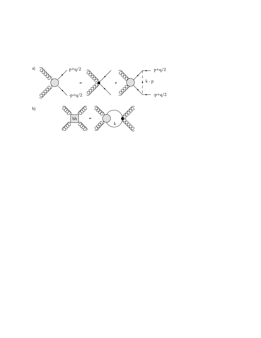
Figure 1: (a) Bethe Salpeter equation for ${\cal M}(gg\rightarrow hh)$ with hidden sector corrections in the ladder aproach (b) Relation between the total scattering amplitude ${\cal M}(gg\underset{hh}{\rightarrow}gg)$ and ${\cal M}(gg\rightarrow hh)$.

Now we can find the amplitude $\mathcal{M}(gg\underset{hh}{\rightarrow}gg)$ by solving the integral equation depicted in Figure (1b):

$$\mathcal{M}(gg\underset{hh}{\rightarrow}gg) = \Gamma^{(0)}(E)$$

$$\int\frac{d^{4}k}{\left(2\pi\right)^{4}}\;\frac{i}{(q/2+k)^{2}-m_{h}^{2}-im_{h}\Gamma_{h}}\;\frac{i}{(q/2-k)^{2}-m_{h}^{2}-im_{h}\Gamma_{h}}\;\Gamma(q,k)$$

Following similar steps as in the previous calculation we obtain

$$\mathcal{M}\left(gg\underset{hh}{\rightarrow}gg\right)=\left(\Gamma^{(0)}(E)\right)^{2}G_{V}(0,E).$$ (9)

Therefore the cross section with the contribution from the hidden sector is

$$\sigma(gg\rightarrow hh)=\sigma_{0}(gg\rightarrow hh)R(E)$$ (10)

with the enhancement factor $R(E)$ is given by

$$R(E)=\frac{\mbox{Im}G_{V}(\vec{0},E)}{\mbox{Im}G_{0}(\vec{0},E)}$$ (11)

where $E=\sqrt{s}-2m_{h}$ is the center-of-mass energy of the Higgsium from threshold and $G_{0}$ is the solution of the same Schroedinger equation (6) in the absence of a potential.

3 Finding the enhancement factor

The solution to eq.(6) can be obtained following the standard procedure of defining two independent solutions $v_{1}$ and $v_{2}$ of the corresponding radial homogeneous equation in the relevant case of zero angular momentum, one regular at the origin and the other regular at infinity:

$$G\left(r,r^{\prime},E+i\Gamma_{h}\right)=\left\{\begin{array}[]{c}-\frac{m_{h}}{4\pi}\frac{v_{1}\left(r\right)v_{2}\left(r^{\prime}\right)}{rr^{\prime}}\ \ \ \ \mbox{for}\ 0<r<r^{\prime}<\infty\\ -\frac{m_{h}}{4\pi}\frac{v_{1}\left(r^{\prime}\right)v_{2}\left(r\right)}{rr^{\prime}}\ \ \ \ \mbox{for}\ 0<r^{\prime}<r<\infty\;,\end{array}\right.$$ (12)

where $v_{1,2}(r)$ is a solution of the equation:

$$\left[\frac{d^{2}}{dr^{2}}+m_{h}\left(E+i\Gamma_{h}-V(r)\right)\right]v(r)=0$$ (13)

We use the method described in Strassler and Peskin [9] to numerically solve the equation above with the appropriate boundary conditions. We will use the functions $v_{a}$ and $v_{b}$ with boundary conditions $v_{a}\left(r\rightarrow 0\right)=r$ and $v_{b}\left(r\rightarrow 0\right)=1$ to write

$$v_{1}(r) = v_{a}(r)$$ (14)

$$v_{2}(r) = v_{b}(r)+Bv_{a}(r).$$ (15)

Hence $B=\underset{r\rightarrow\infty}{\lim}\left(-\frac{v_{b}\left(r\right)}{v_{a}\left(r\right)}\right)$ and we can formally calculate the imaginary part of the Green function as :

$$\mbox{Im}G_{V}(0,0,E+i\Gamma_{h})=-\frac{m_{h}}{4\pi}\mbox{Im}B$$ (16)

In our numerical solution the boundary conditions for the Green function is of course calculated at a finite value of $r$, and it is very important to keep the Higgs boson width that guarantees its exponential decay.

In the absence of a potential it is easy to find that

$$G_{0}\left(r,r^{\prime},E+i\Gamma_{h}\right)=-\frac{m_{h}}{4\pi}\frac{\sin\left(\lambda r\right)}{\lambda r}\frac{e^{i\lambda r}}{r}$$ (17)

where $\lambda=\sqrt{m(E+i\Gamma_{h})}$ and therefore

$$\mbox{Im}G_{0}\left(0,0,E+i\Gamma_{h}\right)=-\frac{m_{h}}{4\pi}\mbox{Re}{\lambda}.$$ (18)

4 Results and Conclusion

We use the results of Plehn et al. [14] to evaluate the cross section without hidden sector corrections , which can be written as:

$$\sigma_{0}(gg\rightarrow hh)=\frac{1}{16\pi s}\left|\mathcal{M}(gg\rightarrow hh)\right|^{2}\sqrt{\left(1-\frac{4m_{h}^{2}}{s}\right)}.$$ (19)

Part of the kinematical factor is cancelled by the denominator of the enhancement factor of eq.(10) resulting in a total cross section given by

$$\sigma(gg\rightarrow hh)=\frac{1}{16\pi s}\left|\mathcal{M}(gg\rightarrow hh)\right|^{2}\sqrt{\left(1+\frac{2m_{h}}{\sqrt{s}}\right)}\;\frac{\mbox{Im}B}{\sqrt{m_{h}\sqrt{s}}}$$ (20)

The enhancement depends basically on two parameters: the strenght of the interaction $\kappa=\frac{g^{2}u^{2}}{8m_{h}^{2}}$ and its range determined by the mass $m_{\phi}$ of the exchanged boson. For $m_{\phi}=0$ one is back to the well known Coulomb case. As an illustration of this effect we will set the Higgs mass in 180 GeV (we checked that our results are weakly dependent on the Higgs mass in the intermediate range).

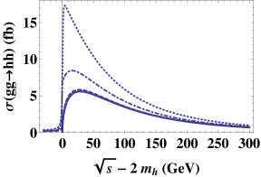
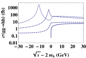
Figure 2: Double higgs production cross section as a function of energy above threshold for $m_{\phi}=50$ GeV. Left panel: Double higgs production cross section cross for $\kappa=0.01,0.1,\;\mbox{and}\;0.3$ (dashed, dot-dashed and dotted lines, respectively) compared with the uncorrected result (solid line). Right panel: Double higgs production cross section near threshold for $\kappa=0.1,0.7,\;\mbox{and}\;1$ (dashed, dot-dashed and dotted lines, respectively) compared with the uncorrected result (solid line). Notice the logarithm scale in this case.

In Figure (2) we show the total cross section $\sigma(gg\rightarrow hh)$ for different values of the coupling constant for $m_{\phi}=50$ GeV. For couplings $\kappa<0.01$ hardly any modification is observed. The difference below threshold is due to the finite width effects contained in the function $G$, which allows a nonzero cross section below threshold. We have checked that our numerical code reproduces the analytical result eq.(18) to high accuracy.

The enhancement increases with the coupling and for values $\kappa>0.6$ a dramatic difference results from the presence of peaks due to Higgs-Higgs bound states. We find enhancement factors as large as a factor of ${\cal O}(100)$ in this case, which is comparable to what has been found in the study of Sommerfeld enhancement for dark matter annihilation cross section in several models [5].

A couple of comments are in order. First, it is a textbook exercise [16] to implement a variational method to estimate the energy of the l=0 bound state in a Yukawa potential. In our case the energy is given by:

$$E=-\kappa m_{\phi}p^{3}(p-1)/4(p+1)^{3}$$ (21)

where p is a solution of the equation $\kappa m_{h}/m_{\phi}=(p+1)^{3}/p(p+3)$. For $\kappa=1$, $m_{h}=180$ GeV and $m_{\phi}=50$ GeV, the values used in our paper, we obtain $E=-11$ GeV ($E=-1.8$ GeV for $\kappa=0.7$). These are in good agreement with our numerical results shown in Figure(2) and corroborate that the bound states are nonrelativistic, since the binding energy is much smaller than the Higgs mass even for these large values of kappa. Secondly, the nonrelativistic approximation is only valid for a region of $30$ GeV or so around threshold. The left plot of Figure(2) is only meant to illustrate that the corrections are small even at high energies. In our numerical results for the LHC cross sections below we switched-off the bound state corrections at an energy of $15$ GeV above threshold.

For lighter $\phi$ masses (${\cal O}(10)$ GeV) the peaks appear for smaller couplings at lower energies and occasionally more than one peak can be seen. For heavier masses, as expected, bound states are not formed but some enhancement effect is still obtained.

In order to estimate the corresponding enhancement at the LHC, we have convoluted the parton level cross section with the gluon distribution function in the proton. For our estimates we used the Mathematica package of the leading order CTEQ5 [17] with factorization and renormalization scales set to $q=2m_{h}$. In Table (1) we present our results for $\sqrt{s}=7$ and $14$ TeV. The convolution smooths out the large partonic enhancements but one can still find cross sections that are as large as 20 times the SM result for extreme values of the coupling. We find that the enhancement factors are not very sensitive to the CM energy, although the absolute values of the production cross section certainly are.

$\kappa$	$\sqrt{s}=7$ TeV	$\sqrt{s}=14$ TeV
0.1	1.1	1.2
0.3	1.5	1.6
0.7	5.5	6.0
1.0	19	21

Table 1: Enhancement factor for double Higgs production cross section at the LHC for different values of the coupling $\kappa$ to a hidden sector for $\sqrt{s}=7$ and $14$ TeV

At this point we should note that the simplest model with an additional singlet would not result in a large enhancement due to the mixing between the scalars, which requires $\kappa<\frac{\lambda m_{\phi}^{2}}{4m_{h}^{2}}$ where $\lambda$ is the Higgs boson self-coupling [18]. There are a few examples where one could have a strong interaction of the hidden sector with the Higgs boson, such as considering a more evolved scalar sector or even interactions with hidden abelian gauge fields or a condensate of fermions. We take no position on what the primary motivation might exist for the hidden sector. Our goal is to consider the general effect of this hidden sector on double Higgs production near threshold.

One may also be concerned with unitarity violation when large couplings are present. For example, at low energies one gets a s-channel contribution to the $s$-wave scattering amplitude that goes as $a_{0}=g^{2}u^{2}/32\pi m_{\phi}^{2}$; this is less than one for $g^{2}u^{2}={\cal O}(m_{h}^{2})$ and the examples discussed here.

The prospects for detection of such an enhancement require a detailed study that is beyond the scope of this short letter. The signal would probably be an excess of 4 gauge boson events near the double Higgs threshold, where the SM background is small. It is amusing to entertain the idea that an investigation of the double Higgs cross section near threshold could lead to important information about the hidden sector.

References

- [1] M. J. G. Veltman and F. J. Ynduráin, Nucl. Phys. B 325, 1 (1989).
- [2] See e.g., G. Bertone, D. Hooper and J. Silk, Phys. Rept. 405, 279 (2005).
- [3] For a recent review, see e.g., J. L. Feng, arXiv:1003.0904.
- [4] J. McDonald, Phys. Rev. D 50, 3637 (1994); C. P. Burgess, M. Pospelov and T. ter Veldhuis, Nucl. Phys. B 619, 709 (2001); M. C. Bento, O. Bertolami, R. Rosenfeld, L. Teodoro, Phys. Rev. D 62, 041302 (2000); M. C. Bento, O. Bertolami, R. Rosenfeld, Phys. Lett. B 518, 276 (2001).
- [5] A. Sommerfeld, Annalen der Physik 403, 257 (1931); A. D. Sakharov, Zh. Eksp. Teor. Fiz. 18, 631 (1948) (reprinted in Sov. Phys. Usp. 34, 375 (1991)); J. Hisano, S. Matsumoto and M. M.Nojiri, Phys. Rev. Lett. 92, 031303 (2004); J. Hisano, S. Matsumoto, M. M.Nojiri and O. Saito, Phys. Rev. D 71, 063528 (2005); R. Iengo, JHEP 05, 024 (2009).
- [6] See, e.g., M. Cirelli, A. Strumia and M. Tamburini, Nucl. Phys. B 787, 152 (2007); N. Arkani-Hamed, D. P. Finkbeiner, T. R. Slatyer and N. Weiner, Phys. Rev. D 79 015014 (2009); J. D. March-Russell and S. M. West, Phys. Lett. B 676, 133 (2009); M. Lattanzi and J. Silk, Phys. Rev. D 79, 083523 (2009); M. R. Buckley and P. J. Fox, Phys. Rev. D 81, 083522 (2010); J. L. Feng, M. Kaplighat and H.-B. Yu, arXiv:1005.4678.
- [7] C. Arina, F. Josse-Michaux and N. Sahu, Phys. Rev. D 82, 015005 (2010).
- [8] See, e.g., C. O. Dib, R. Rosenfeld and A. Zerwekh, JHEP 0605 074 (2006); H. de Sandes and R. Rosenfeld, Phys. Lett. B 659, 323 (2008); E. Asakawa et al., arXiv:1009.4670.
- [9] V. S. Fadin and V A. Khoze, JETP Lett. 46, 525 (1987); V. S. Fadin, V A. Khoze and T. Sjostrand, Z. Phys. C48, 613 (1990); M. J. Strassler and M. E. Peskin, Phys. Rev. D 43, 1500 (1991); K. Hagiwara, Y. Sumino and H. Yokoya, Phys. Lett. B 666, 71 (2008); Y. Kiyo, J. H. Kühn, S. Moch, M. Steinhauser and P. Uwer, Eur. Phys. J. C 60, 375 (2009); Y. Sumino and H. Yokoya arXiv:1007.0075v1.
- [10] Y. Kats and M. D. Schwartz, JHEP 1004, 016 (2010).
- [11] J. A. Grifols, Phys. Lett. B 264, 149 (1991).
- [12] B. Grinstein and M. Trott, Phys. Rev. D 76, 073002 (2007).
- [13] R. N. Cahn and M. Suzuki, Phys. Lett. B 134, 115 (1984); A. P. Contogouris, N. Mebarki, D. Atwood and H. Tanaka, Mod. Phys. Lett. A 3, 295 (1988); G. Rupp, Phys. Lett. B 288, 99 (1992).
- [14] T. Plehn, M. Spira and P. M. Zerwas, Nucl. Phys. B 479, 46 (1996).
- [15] For a nonperturbative study of bound states in a model similar to ours, see T. Niewenhuis and J. A Tjon, Phys. Rev. Lett. 77, 814 (1996).
- [16] S. Flügge, Practical Quantum Mechanics, Springer Verlag (1971).
- [17] CTEQ Collaboration (H. L. Lai et al.), Eur. Phys. J. C 12, 375 (2000).
- [18] R. Schabinger and J. D. Wells, Phys. Rev. D 72, 093007 (2005).