Using epidemic prevalence data to jointly estimate reproduction and removal

Abstract

This study proposes a nonhomogeneous birth–death model which captures the dynamics of a directly transmitted infectious disease. Our model accounts for an important aspect of observed epidemic data in which only symptomatic infecteds are observed. The nonhomogeneous birth–death process depends on survival distributions of reproduction and removal, which jointly yield an estimate of the effective reproduction number $R(t)$ as a function of epidemic time. We employ the Burr distribution family for the survival functions and, as special cases, proportional rate and accelerated event-time models are also employed for the parameter estimation procedure. As an example, our model is applied to an outbreak of avian influenza (H7N7) in the Netherlands, 2003, confirming that the conditional estimate of $R(t)$ declined below unity for the first time on day 23 since the detection of the index case.

and

1 Introduction

The data-generating process of an epidemic has special characteristics to which one wants to pay particular attention when modeling these data. First, the observed data of an infectious disease outbreak are limited in the sense that the incidence—expressed as the number of newly infected individuals as a function of time—is usually measured by symptom onset of disease, which is sometimes further accompanied by reporting delay. Thus, all of the observed cases in the reported data represent those who experienced infection at some point in time in the past. Second, epidemic data sets do not usually include information on the number of susceptible individuals as a function of time, but solely records infected (interpreted as symptomatic) individuals. It is therefore unknown if susceptible individuals in the past are still susceptible at a point of time. Third, the susceptible population is usually not well defined at the beginning of an outbreak, and its size may vary with time due to time-dependency in contact behavior and public health countermeasures during the outbreak. In a veterinary context, the countermeasures might include a transportation ban during an infectious disease outbreak on animal farms. Control measures are taken not only to reduce the number of contacts, but also to limit the ability of infected individuals to generate secondary cases. For instance, one may think of preemptive culling in the case of an infectious disease outbreak on animal farms. Fourth, since the infection is transmitted from individual to individual, observation of an infected individual is not independent of observing other individuals.

These characteristics lead us to consider developing a method which appropriately captures the dynamics of a directly transmitted infectious disease by modeling the number of infected-and-detected individuals, preferably in discrete time, in order to quantify the reproduction of infected individuals in a nonhomogeneous manner. This contrasts with other statistical models which measure the population of susceptibles and model the force of infection at which these susceptibles get infected.

As is usually assumed, one can think of a population in which an epidemic of an infectious disease occurs as consisting of three groups (or sub-populations) of individuals. The first is the susceptible population which represents individuals who have not been infected yet but may experience infection in the future. The second is a population of infectious individuals which consists of those who have been infected and are infectious to others. The last group consists of removed or recovered individuals who are no longer infectious and may be immune or are removed from the population. The simplest type of the model which describes the transmission dynamics over time is referred to as an SIR (Susceptible-Infected-Recovered) model [Diekmann and Heesterbeek (2000)]. Since the present study will concentrate on the number of infected, here we consider their dynamics alone. Letting $x(t)$ and $y(t)$ be the susceptible and infectious fractions of the population at time $t$, respectively, the derivative of $y(t)$ is expressed as

$$\frac{\mathrm{d}}{\mathrm{d}t}y(t)=\beta(t)y(t)x(t)-\mu(t)y(t).$$ (1)

Note that the transmission rate $\beta(t)$ and the removal rate $\mu(t)$ may depend on time. If one rewrites the product of the transmission rate $\beta(t)$ and susceptibles $x(t)$ as $\lambda(t)$ ($=\beta(t)x(t)$), then the equation is rewritten as

$$\frac{\mathrm{d}}{\mathrm{d}t}y(t)=\lambda(t)y(t)-\mu(t)y(t),$$ (2)

which is the equation of the deterministic nonhomogeneous birth–death process. The function $\lambda(t)$ has been referred to as the reproductive power and can be interpreted as the rate at which a single infected individual is able to generate secondary cases [Kendall (1948)]. In other words, $\lambda(t)$ is the rate at which an infected individual is able to reproduce itself. The so-called death rate $\mu(t)$ in a birth–death process is interpreted as the rate at which an infected individual is removed from the sub-population of infected individuals. It should be noted that equation (2) relaxed the definition of $y(t)$ compared to that in (1). Namely, whereas $y(t)$ in (1) has to be infectious to others, we can instead regard $y(t)$ in (2) as infected-and-detected individuals (i.e., regardless of infectiousness).

One of the advantages of using this simple equation is that the population of susceptibles is allowed to vary over time. Therefore, the reproductive power varies over time due to two different reasons: (1) the population of susceptibles $x(t)$ varies as a function of time and (2) the transmission rate $\beta(t)$ is nonhomogeneous over time. In addition, the removal rate $\mu(t)$ is allowed to vary with time.

It can be an advantage to model infection process stochastically, because one can explicitly define the probability of transmission, rather than deterministically stating if the transmission happens [Andersson and Britton (2000)]. A stochastic model can describe not only the quantitative patterns of observation with time-dependent expected values, but also offer standard errors of the parameters without making adhoc distributional assumptions. More importantly, the likelihood function can be explicitly derived, which will be useful for statistical inference of parameters and critical assessments of the modeling method. Moreover, such a stochastic process can model the number of infected over time as being dependent.

The present study aims to develop a stochastic model which is based on a nonhomogeneous birth–death process. The model is applied to an observed data set of infected-and-detected (but not yet removed) cases, permitting reasonable assessment of the time course of an epidemic. In Section 2 the stochastic version of the nonhomogeneous birth–death model is comprehensively described. A novel analytical solution of the model is obtained with the use of a general Lagrange transformation derivation of which has not been explicitly discussed to date. In Section 3 we discuss a conditional discrete-time fitting method. Although a similar conditional fitting procedure was employed in a recent study [van den Broek and Heesterbeek (2007)], the present study is the first to apply the technique to a model where both birth and death rates are nonhomogeneous. Depending on the model and the data given, the number of parameters to be estimated can be large and it might be difficult to get stable estimates. Besides, a relationship between the reproductive power and the removal rate might exist. Therefore, more restricted models which employ this relationship are discussed in Section 4. In Section 5 our model is applied to an observed epidemic data set of avian influenza A (H7N7) in the Netherlands, 2003.

2 The nonhomogeneous birth–death model

The stochastic differential equations for a nonhomogeneous birth–death process, with $Y(t)$ and $y_{0}$ being the number of infected-and-detected at time $t$ and the initial number of infected-and-detected at time $0$, respectively, are as follows:

$$\frac{\mathrm{d}}{\mathrm{d}t}p_{y}(t) = \lambda(t)(y-1)p_{y-1}(t)+\mu(t)(y+1)p_{y+1}(t)-\bigl{(}\lambda(t)+\mu(t)\bigr{)}yp_{y}(t),$$

$$\frac{\mathrm{d}}{\mathrm{d}t}p_{0}(t) = \mu(t)p_{1}(t),$$

where $\lambda(t)$ denotes the reproductive power, $\mu(t)$ the death rate and $\Pr(Y(t)=y)=p_{y}(t)$ the probability that the number of infected-and-detected individuals at time $t$ is $y$. It should be noted that here we consider $Y(t)$ as the number of infected-and-detected individuals which represents the observed elements of the data and is irrelevant to infectiousness. If we take the probability generating function of the probabilities $p$, we can derive a partial differential equation for this fraction by multiplying the above differential equations with $z^{y}$, summing the result, and taking the derivative. The analytical solution of the partial differential equation is [Kendall (1948)]

$$\Phi(y,u)=\biggl{[}\frac{\theta-(1-\pi-\theta)u}{1-\pi u}\biggr{]}^{y_{0}}.$$

If we write $\rho(t)=\int_{0}^{t}[\mu(\tau)-\lambda(\tau)]\,\mathrm{d}\tau=\log[\frac{S_{\lambda}(t)}{S_{\mu}(t)}]$ and

$$\gamma(t)=\int_{0}^{t}e^{\rho(\tau)}\lambda(\tau)\,\mathrm{d}\tau=-\int_{0}^{t}\frac{\mathrm{d}S_{\lambda}(\tau)}{S_{\mu}(\tau)},$$ (3)

we get

$$\theta = 1-\frac{e^{-\rho(t)}}{1+\gamma(t)e^{-\rho(t)}}=1-\frac{S_{\mu}(t)}{S_{\lambda}(t)+\gamma(t)S_{\mu}(t)},$$ (4)

$$\pi = 1-\frac{1}{1+\gamma(t)e^{-\rho(t)}}=1-\frac{S_{\lambda}(t)}{S_{\lambda}(t)+\gamma(t)S_{\mu}(t)}.$$ (5)

It should be noted that $S_{\lambda}(t)=e^{-\int_{0}^{t}\lambda(\tau)\,\mathrm{d}\tau}$ is the reproduction survival function and $S_{\mu}(t)=e^{-\int_{0}^{t}\mu(\tau)\,\mathrm{d}\tau}$ is the removal survival function.

To obtain the probability distribution from $\Phi(y,u)$, the general Lagrange transformation is useful (the details of which can be found elsewhere[Consul and Famoye (2006)]). First, let $\Phi(y,u)=[\theta+(1-\theta)\frac{(1-\pi)u}{1-\pi u}]^{y_{0}}=[\theta+(1-\theta)\psi(u)]^{y_{0}}$, where $\psi(u)$ is the probability generating function (pgf) of the geometric distribution. Second, let $g(z)=1-\pi+\pi z$, the pgf of a Bernoulli distribution. Numerically, the smallest root of the transformation $z=ug(z)$ defines a pgf $z=\psi(u)=\frac{(1-\pi)u}{1-\pi u}$ [Consul and Famoye (2006)]. Third, additionally considering $f(z)=(\theta+(1-\theta)z)^{y_{0}}$, the pgf of the discrete general Lagrange probability distribution under the Lagrange transform $z=ug(z)$ is given by $f(z)=f(\psi(u))=[\theta+(1-\theta)\frac{(1-\pi)u}{1-\pi u}]^{y_{0}}$ and, moreover, the probability mass function is a special case of the double-binomial distribution [Consul and Famoye (2006), pages 22–27], which can be referred to as the Bernoulli-binomial Lagrangian distribution in the terminology of [Johnson, Kemp and Kotz (2005)]

$$P\bigl{(}Y(t)=0\bigr{)} = \theta^{y_{0}},$$

$$P\bigl{(}Y(t)=y\bigr{)} = \frac{y_{0}}{y}\theta^{y_{0}}\pi^{y}\sum_{k=0}^{\min(y-1,y_{0}-1)}\pmatrix{y_{0}-1\cr k}\pmatrix{y\cr y-k-1}$$

$$\hphantom{\frac{y_{0}}{y}\theta^{y_{0}}\pi^{y}\sum_{k=0}^{\min(y-1,y_{0}-1)}}{}\times\biggl{[}\frac{(1-\pi)(1-\theta)}{\pi\theta}\biggr{]}^{k+1},$$

$$\hskip 223.0pty\geq 1,$$

where $\theta$ and $\pi$ are defined in equations (4) and (5). It should be noted that $g(z)$ and $f(z)$ are pgf’s and, thus, the necessary conditions for Lagrange transformation are satisfied. To the best of our knowledge, detailed derivation of equation (2) has never been discussed in the context of the nonhomogeneous birth–death model (see Section 6).

The expectation and the variance of (2) are

$$E(y) = y_{0}\frac{1-\theta}{1-\pi}$$

$$= y_{0}\frac{S_{\mu}(t)}{S_{\lambda}(t)},$$

$$\operatorname{var}(y) = y_{0}\frac{(1-\theta)[\theta+\pi(1-\theta-\pi)]}{(1-\pi)^{3}}$$

$$= y_{0}\frac{S_{\mu}(t)}{S_{\lambda}(t)}\biggl{[}1+(2\gamma-1)\frac{S_{\mu}(t)}{S_{\lambda}(t)}\biggr{]}$$

$$= y_{0}R(t)[1+(2\gamma-1)R(t)]$$

by using (4) and (5).

The expected value has two interpretations. The first part is the predicted number of infected individuals at time $t_{0}$ who survived removal [i.e., $y_{0}S_{\mu}(t)$]. The second part, $\frac{1}{S_{\lambda}(t)}$, measures the rate at which a nonremoved infected individual reproduces itself. This is similar to an interpretation of a nonhomogeneous birth process [van den Broek and Heesterbeek (2007)]; the difference of the present study from the previous nonhomogeneous birth process is that in the present setup only the predicted nonremoved infected-and-detected individuals reproduce. Second, the ratio of the rates $\frac{S_{\mu}(t)}{S_{\lambda}(t)}$ is the net reproduction ratio with which an infected individual reproduces itself, which is interpreted as the effective reproduction number $R(t)$ as a function of epidemic time $t$. $R(t)$ in the present study can be regarded as the average number of secondary cases generated by a single primary case at time $t$. That is, our $R(t)$ is an instantaneous measure of secondary transmissions occurring at time $t$, whose definition is equivalent to the period total fertility rate in mathematical demography [Nishiura and Chowell (2009)]. If $R(t)<1$, it suggests that the epidemic is in decline and may be regarded as being “under control” at time $t$ [vice versa, if $R(t)>1$]. It should be noted that the expected value of (2) is equivalent to an analytical solution of the deterministic version of a nonhomogeneous birth–death process (2).

The term $\gamma(t)$ in the formula for the variance represents the dependence between the birth and death rate as can be seen from (3). As it is clear from the analytical expression for the variance, the variance becomes large if the probability of nonremoval is large for an infected individual, if the probability of reproduction is large, or both. This matches intuitive sense. In addition, the variance can be regarded as a type of negative binomial variance, if we rewrite it as $\operatorname{var}(y)=E(y)[1+\frac{2\gamma-1}{y_{0}}E(y)]$.

3 Fitting the model

We have shown how the epidemic data can be generated by a stochastic nonhomogeneous birth–death process. Nevertheless, the observed data are, in reality, just one sample path of all the possible sample paths that can arise from such an epidemic process. Considering further that the number of infected-and-detected and individuals at a certain point in time $t$ depends on the number of infected-and-detected individuals at some time point before $t$, our model is fitted to the data by conditioning on the transmission dynamics which happened before $t$ [Becker (1989), Becker and Yip (1989)]. Moreover, as we briefly discussed in the Introduction, another important point in practice is the discrete nature of the time points of observation, that is, say, $t_{j}$, $j=0,1,\ldots,n$, where the time unit might typically be days or weeks. Therefore, the number of infecteds at time $t_{j}$ is modeled conditionally on the number of infecteds by time $t_{j-1}$.

Since the probability mass function (2) is a conditional probability mass function, conditioning being on the number of infecteds at $t_{0}$, this can be effectively used as the conditional model for the number of infecteds at time $t_{j}$, given the number of infecteds at time $t_{j-1}$. For this reason, the survival distributions $S_{\lambda}(t)$ and $S_{\mu}(t)$ and, of course, $\gamma(t)$, are also conditioned on the past. Let $T_{\lambda}$ and $T_{\mu}$ be the stochastic variables that measure the reproduction time and the removal time, respectively. The conditional survival probability for the reproduction time is

$$P(T_{\lambda}>t_{j}|T_{\lambda}>t_{j-1}) = \frac{S_{\lambda}(t_{j})}{S_{\lambda}(t_{j-1})}$$

$$= 1-\frac{S_{\lambda}(t_{j-1})-S_{\lambda}(t_{j})}{S_{\lambda}(t_{j-1})}$$

$$= 1-P\bigl{(}T_{\lambda}\in(t_{j-1},t_{j}]|T_{\lambda}>t_{j-1}\bigr{)}$$

$$= 1-h_{\lambda}(t_{j-1}),$$

where $h_{\lambda}(t_{j-1})$ is interpreted as the discrete reproductive power. Similarly, the conditional survival probability for the removal time is given by

$$P(T_{\mu}>t_{j}|T_{\mu}>t_{j-1})=1-h_{\mu}(t_{j-1}),$$

where $h_{\mu}(t_{j-1})$ is the discrete removal hazard.

The discrete conditional version of (3) in the time interval ($t_{j-1}$, $t_{j}$] is

$$\frac{P(T_{\lambda}\in(t_{j-1},t_{j}]|T_{\lambda}>t_{j-1})}{P(T_{\mu}>t_{j}|T_{\mu}>t_{j-1})}=\frac{h_{\lambda}(t_{j-1})}{1-h_{\mu}(t_{j-1})}.$$

When these conditional discrete measurements are considered, $\theta$ and $\pi$ correspond to $h_{\mu}(t_{j-1})$ and $h_{\lambda}(t_{j-1})$, respectively. Using these, the conditional probability for (2) is expressed as

$$P\bigl{(}Y(t_{j})=0|Y(t_{j-1})=y_{t_{j-1}}\bigr{)}=h_{\mu}(t_{j-1})^{y_{0}},\vspace*{-6pt}$$

$$P\bigl{(}Y(t_{j})=y_{t_{j}}|Y(t_{j-1})=y_{t_{j-1}}\bigr{)}$$

$$\qquad=\frac{y_{t_{j-1}}}{y_{tj}}h_{\mu}(t_{j-1})^{y_{t{j-1}}}h_{\lambda}(t_{j-1})^{y_{t_{j}}}$$

$$\quad\qquad{}\times\sum_{k=0}^{\min(y_{t_{j}}-1,y_{t_{j-1}}-1)}\pmatrix{y_{t_{j-1}}-1\cr k}\pmatrix{y_{t_{j}}\cr y_{t_{j}}-k-1}$$

$$\hphantom{\quad\qquad{}\times\sum_{k=0}^{\min(y_{t_{j}}-1,y_{t_{j-1}}-1)}}{}\times\biggl{[}\frac{(1-h_{\lambda}(t_{j-1}))(1-h_{\mu}(t_{j-1}))}{h_{\lambda}(t_{j-1})h_{\mu}(t_{j-1})}\biggr{]}^{k+1},\qquad y\geq 1.$$

The expected value of this probability is $y_{t_{j-1}}\frac{1-h_{\mu}(t_{j-1})}{1-h_{\lambda}(t_{j-1})}$, which is referred to as the sample path profile [Lindsey (2001)]. The corresponding conditional measurement of the effective reproduction number is $R(t_{j-1})=\frac{1-h_{\mu}(t_{j-1})}{1-h_{\lambda}(t_{j-1})},$ with $h_{\mu}(t_{j-1})=1-\frac{S_{\mu}(t_{j})}{S_{\mu}(t_{j-1})}$ and $h_{\lambda}(t_{j-1})=1-\frac{S_{\lambda}(t_{j})}{S_{\lambda}(t_{j-1})}$.

Let $\Delta$ be the vector of parameters from the survival distributions (see Section 4). The log-likelihood function is then

$$l(\Delta)=\sum_{i=1}^{n}\log\bigl{[}P\bigl{(}Y(t_{j})=y_{t_{j}}|Y(t_{j-1})=y_{t_{j-1}},\Delta\bigr{)}\bigr{]}.$$

Note that the likelihood is evaluated only for $y_{t_{j}}>0$, because zero prevalence is the absorbing state of the process and this state is not observable in reality.

The log-likelihood can be maximized using an optimization procedure, such as the Nelder–Mead method to find the maximum likelihood estimates. In our exercise, the software system R [R Development Core Team (2008)] is used. The information matrix is used to find the standard errors of the parameters, and we use Akaike’s information criterion (AIC) to compare model fits.

4 The Burr distribution and its special cases

To choose a particular form for the survival functions, one might take the early phase of the outbreak into account. The mean of the probability mass function (2) depends on these survival functions and is the same as the solution of (2). Since (2) can be derived from the SIR model, one might look at the deterministic SIR-model to decide the parametric form of the survival function. In the early phase of the outbreak a deterministic SIR-model can be well approximated by a deterministic SI-model since in that phase the number of removals is limited. The dynamic equations for this SI-model hold for the fraction of susceptibles and for the fraction of infected and since the fraction of susceptibles at a point of time is the same as the fraction of individuals with infection time larger than that time point, the dynamic equations should also hold for the survival function. The Burr family of distribution functions has this precise property [van den Broek and Heesterbeek (2007)].

When detection of a symptomatic infected individual occurs, he/she usually will be removed immediately. Thus, it is reasonable to assume that the reproductive power and the removal rate have a similar structure, and follow a similar survival function.

The most well-known and useful distribution from the Burr family is the Burr XII, or Singh–Maddala distribution, which in the literature is sometimes referred to simply as the Burr distribution. The survival function is given by

$$S(t)=\biggl{[}1+\biggl{(}\frac{t}{b}\biggr{)}^{a}\biggr{]}^{-q},\qquad t>0,a,b,q>0.$$

The right tail is governed by the parameters $a$ and $q$, the left tail by $a$, and $b$ is the scale parameter [Kleiber and Kotz (2003), page 198]. To reduce the number of parameters to be estimated, one can consider three special cases of the Burr distribution [Kleiber and Kotz (2003)]:

1. The logistic form is obtained for $q=1,$ giving the log-logistic or the Fisk distribution.

2. For $a=1$, the Burr distribution is reduced to the Lomax (Pareto type II) distribution.

3. The case $a=q$ is also known as the para-logistic distribution.

The Weibull distribution and the Pareto distribution are limiting cases of the Burr distribution [Shao (2004)]. An interesting way to arrive at the Burr distribution is to assume that the times follow a Weibull distribution, the scale parameter of which follows an inverse generalized gamma distribution [Kleiber and Kotz (2003)].

As another way to reduce the number of model parameters, and to find a further relationship between the reproductive power and the removal rate, one may rewrite the Burr distribution as a proportional rate or an accelerated event-time distribution (just as in the case of the more famous Weibull distribution). Suppose that the survival function for the reproduction time is a Burr distribution with parameters $a,b_{1}$ and $q$ and suppose that the survival function of the removal time is also a Burr distribution with parameters $a,b_{2}$ and $q$. If we replace $b_{2}$ by $db_{1}$ (where $d$ is a constant), we get

$$S_{\mu}(t)=\biggl{[}1+\biggl{(}\frac{t}{b_{2}}\biggr{)}^{a}\biggr{]}^{-q}=\biggl{[}1+\biggl{(}\frac{t}{db_{1}}\biggr{)}^{a}\biggr{]}^{-q}=\biggl{[}1+\biggl{(}\frac{t^{\prime}}{b_{1}}\biggr{)}^{a}\biggr{]}^{-q}=S_{\lambda}(t^{\prime}).$$

Therefore, the survival distribution for the removal times is exactly the same as that for the reproduction time, except that the removal time is interpreted as accelerated reproduction time.

To employ the proportional rate model, let the survival distribution for the reproduction time be a Burr distribution with parameters $a,b$ and $q_{1}$, and suppose that the survival distribution of the removal times is also a Burr distribution with parameters $a,b$ and $q_{2}$. If we replace $q_{2}$ by $cq_{1}$ (where $c$ is a constant), we get

$$S_{\mu}(t)=\biggl{[}1+\biggl{(}\frac{t}{b}\biggr{)}^{a}\biggr{]}^{-q_{2}}=\biggl{[}1+\biggl{(}\frac{t}{b}\biggr{)}^{a}\biggr{]}^{-cq_{1}}=\biggl{\{}\biggl{[}1+\biggl{(}\frac{t}{b}\biggr{)}^{a}\biggr{]}^{-q_{1}}\biggr{\}}^{c}=\{S_{\lambda}(t)\}^{c},$$

indicating that the rates are proportional; that is, the rate at which an infected-and-detected is removed is proportional to the rate at which an infected-and-detected individual reproduces. Of course, the Burr distribution can also be written as both an accelerated event-time distribution and as a proportional rate distribution, that is, $S_{\mu}(t)=[S_{\lambda}(t^{\prime})]^{c}$.

All the distributions described above can be written in accelerated event-time form and in proportional hazard form, except for log-logistic distribution which has only an accelerated event-time form. In the next section we fit all of those models to epidemic data of avian influenza A (H7N7) in the Netherlands, 2003.

5 Dutch avian influenza A (H7N7) epidemic in 2003

Here we show an example of our model application to an observed data set. An epidemic of avian influenza A (H7N7) virus started on February 28, 2003, in the Gelderse Vallei in the Netherlands. In total, 239 flocks experienced infection with known detection date. Control measures taken include movement restrictions, stamping out of infected flocks, and preemptive culling of flocks in the neighborhood of infected flocks. As a result, 1255 commercial flocks and 17,421 flocks of smallholders had to be depopulated, and approximately 25.6 million animals were killed. The virus was also transmitted to humans who had been in close contact with the infected chickens, resulting in one human death. Further details can be found elsewhere [Stegeman et al. (2003)].

We examine transmission and detection events between flocks. We regard the detection date of a case (i.e., infected individual) as the date at which there were first signs of infection in a flock. In other words, the detection date of an infected individual is regarded as the birth date in our model. Therefore, the birth date is not the date of infection but the date at which an infected farm is detected, which is used as a surrogate. Moreover, the date of depopulation is regarded as the death date. Consequently, the Dutch data consist of the prevalence of infected-and-detected (but not yet removed) flocks on each epidemic date.

Figure 1 shows the temporal distribution of the prevalent cases (representing those who were born and have not been removed yet). As can be seen, the right tail contains gaps and the center of the distribution is not well determined. Usually these make it difficult to fit simple models to the data.

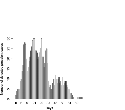
Figure 1: Temporal distribution of the prevalent cases of avian influenza A (H7N7) epidemic in the Netherlands, 2003. The index case was reported on February 28, 2003 (and the date is defined as day 0). The prevalent cases represent those who have been infected and detected but have not been depopulated yet at day $t$, which correspond to the expected value of $y_{t}$ in Section 3. See Stegeman et al. 2003 for further information.

Table 1: Akaike’s information criterion (AIC) for different models

	Full model	Acc. event time[1]table11	Prop. rate[2]table12	Both acc. event and prop. rate
Burr	342.4	345.90	346.4	342.7
Log-logistic	371.3	369.8	–	–
Lomax	341.9	344.8	344.9	same as full model
Para-logistic	351.8	354.0	357.5	same as full model

[1]table11Accelerated event-time model. [2]table12Proportional rate model.

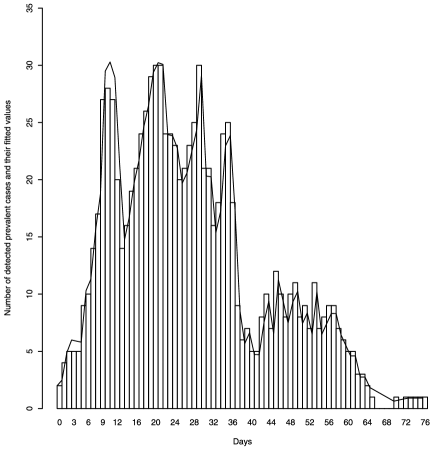
Figure 2: Comparison of the observed numbers and the predicted values from the conditional model of prevalent cases of avian influenza A (H7N7) epidemic in the Netherlands, 2003. The index case was reported on February 28, 2003 (and the date is defined as day 0). Observed data (bars) is compared with the predicted number of cases (solid line) based on the full Lomax model. It should be noted that the expectation of prevalence $y_{t_{j}}$ is conditioned on $y_{t_{j-1}}$.

The Burr model with three parameters for birth rate and three for death rate was fitted to the observed data. We refer to it as the full Burr model. To objectively show how this model fits to the data better than other types of models, we compared its likelihood with that of the full inverse Burr (Burr III or Dagum) model. The inverse Burr model is also known as a flexible distribution from the Burr family and can be viewed as a generalized gamma with a scale parameter that follows an inverse Weibull distribution [Kleiber and Kotz (2003)]. The inverse Burr yielded an AIC of $363.7$, while the full Burr model yielded 342.4. We thus examined the full Burr model (and its special cases) for further analyses. The AICs for these different models are in Table 1. The full Lomax model gave the best fit, although the difference in AIC with the full Burr distribution was not particularly large. In other words, the information criterium suggest that both the death rate and the reproductive power may be proportional and that the removal time may be accelerated reproduction time in the observed data set. Figure 2 visually confirms a good fit of the full Lomax model to the observed number of infected-and-detected individuals based on the conditional model in discrete time. The model seems to have well captured the observation, because fitting prevalence $y_{t_{j}}$ to the data is conditioned on $y_{t_{j-1}}$. It should be noted that the predicted values in Figure 2 reflect a qualitative pattern of the observed data always one or two steps late, which is a general tendency of conditional fit.

=172pt Parameter Estimate St. error $\ln(b_{1})$ 3.235 0.5998 $\ln(q_{1})$ 2.712 0.3611 $\ln(b_{2})$ 4.987 1.0396 $\ln(q_{2})$ 3.980 0.8480

Table 2: Parameter estimates for the Lomax distribution

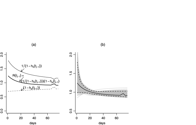
Figure 3: Time dependency of birth and death rates which jointly yield the effective reproduction number. (a) ($(1-h_{\mu}(t_{j-1})$) indicates the rate at which an infected-and-detected case escapes removal, whereas ($1/(1-h_{\lambda}(t_{j-1}))$) denotes the rate at which a single infected-and-detected (but not yet removed) case reproduces secondary cases. The product $(1-h_{\mu}(t_{j-1}))$ $/(1-h_{\lambda}(t_{j-1}))$ yields the effective reproduction number $R(t)$ as a function of time, which can be interpreted as the average number of secondary cases generated by a single primary case at time $t_{j-1}$. If $R(t_{j-1})<1$, it suggests that the epidemic is in decline. In our example, the expected value of $R(t_{j-1})$ declined below unity on day 23 since the detection of index case. (b) The effective reproduction number, $R(t_{j-1})$, calculated from sample paths drawn from the underlying estimated process (gray lines) with the estimated value (black line) and the 95% percentile lines (dashed lines).

Parameter estimates for the best fitting model are shown in Table 2 with their standard errors. The logarithm of the acceleration factor, $d$, was estimated at $1.47$ with a standard error of $0.369$, and the logarithm of the proportionality between the reproductive power and the removal rate was $1.54$ with a standard error of $0.355$. The estimates of mean reproduction and removal times for the Lomax distribution can be calculated from [Kleiber and Kotz (2003)] $E(t)=\frac{b\Gamma(2)\Gamma(q-1)}{\Gamma(q)}$. The mean reproduction time was estimated as $1.81$, indicating that it takes on average 1.8 days for a detected case to reproduce another detected case. The mean removal time was estimated as $2.79,$ indicating that on average it takes 2.8 days for a detected infected case to be removed.

In Figure 3 the rate at which a single case survives removal, ($1-h_{\mu}(t_{j-1})$), is shown as a function of epidemic date. In addition, the rate at which a single nonremoved case reproduces secondary cases, ($1/(1-h_{\lambda}(t_{j-1})$), is also shown in the figure. The product of these two functions jointly yields $R(t_{j-1})$ (also shown in Figure 3). Compared with other modeling results [e.g., Nishiura and Chowell (2009)], our estimates of $R(t_{j-1})$ are smoothed as a function of time owing to our parametric model for the survival functions of reproduction and removal. Nevertheless, it should be noted that our approach does not have to assume that the generation time distribution is known [i.e., common assumption in estimating $R(t)$], because our approach does not have to translate a growth rate of incidence to the reproduction number. As we discussed above, $R(t_{j-1})<1$ suggests that the epidemic is in decline at time $t_{j-1}$ [vice versa, if $R(t_{j-1})>1$]. This can be understood by considering the condition for $R(t_{j-1})=1$; that is, the reproductive power becomes equivalent to the removal rate at time $t$. In our example, the expected value of $R(t_{j-1})$ declined below unity for the first time on day 23 since the detection of the index case, supporting eventual end of the epidemic in the later stage. The sawtooth at the end of the lines is considered to have been caused by zero prevalence during the corresponding time period (i.e., because of our conditional measurement, the survival functions reflect small variations in the observed data). Figure 3(b) shows the estimated effective reproduction number $R(t_{j-1})$. To get an idea of the statistical uncertainty of $R(t_{j-1})$, 500 sample paths were drawn from the estimated nonhomogeneous birth–death model and for each sample path the effective reproduction number was calculated (gray lines). The 95% percentile lines of $R(t_{j-1})$ are also shown.

6 Discussion

In the present study we modeled an epidemic based on the nonhomogeneous birth–death process, addressing some of the critical issues which are seen in the observation of directly transmitted infectious diseases. First, we modeled infected-and-detected individuals, which corresponds to observable and countable information in practice (e.g., our model requires neither susceptibles nor infectious individuals). Second, for a similar reason, the application of a birth–death process allowed the population at risk (i.e., the susceptible population) to vary with time. Third, applying the concepts of a nonhomogeneous birth–death process to epidemic modeling, dependent events (i.e., dependence of a single infected individual on other infected individuals) were addressed in the model. Fourth, our stochastic model offered an explicit likelihood function and yielded a standard error of parameters. Last, our model allowed estimation of the effective reproduction number, $R(t)$. Although a different probability distribution was given by Bailey (1964), the derivation was not given in the literature, and, to the best of our knowledge, equation (2) is the first to derive the pdf explicitly.

In a recent study van den Broek and Heesterbeek (2007) applied a nonhomogeneous birth process to epidemic data, in which the survival-time distribution was modified by a final-size parameter to describe the end of an epidemic (which was influenced by public health countermeasures). The countermeasures would not only reduce the final size of an epidemic but also the reproductive power as a function of time, because secondary transmissions caused by infected individuals are restricted under the control measures. The nonhomogeneous birth process in the previous study permitted an explicit assessment of the time variations in the number of newly infected individuals (and thus the reproductive power).

In the present study the proposed nonhomogeneous birth–death process further improved our understanding of time dependency by explicitly adding the nonhomogeneous removal rate. Whereas the reproductive power changes as a function of time due to variations in susceptible individuals or in the transmission rate, the removal rate is also nonhomogeneous when infected individuals are likely to be removed upon detection. Thus, adding nonhomogeneous death to a nonhomogeneous birth process enabled us to separately consider the effectiveness of countermeasures as a reduction in reproductive power (e.g., reduction in infectious contacts) and an increase in removal rate of infected individuals (e.g., culling of infected farms). In this way, the fading out of an epidemic was modeled in a smoother way, as compared to the previous model based on a nonhomogeneous birth process alone.

Moreover, it should be noted that our model does not necessarily require a homogeneous mixing assumption to describe contacts, because our assumptions of the time-dependent rates implicitly include those nonhomogeneities. For example, our model allows time variations in susceptible individuals. Nevertheless, our model only accounts for the nonhomogeneity with respect to time in an explicit manner, and understanding other heterogeneous aspects of transmission requires further information.

Of course, there are many possible candidate distributions to model the reproduction and the removal times. We have selected the Burr distribution for three reasons:

1. As noted in Section 4, the Burr family coincides with our analytical understanding of the epidemic modeling, especially at the early stage of an epidemic.

2. Essentially, the Burr distribution is flexible and has special and limiting cases. For instance, the distribution can be regarded as a Weibull distribution with a random scale parameter.

3. In the context of the present study, the proportional hazard rate and the accelerated event time interpretation may be very helpful in model reduction and further interpretation of the data.

As an example, the nonhomogeneous birth–death model was applied to epidemic data of avian influenza A (H7N7) in the Netherlands, 2003, showing that the model fitted to the data very well. Indeed, since the data set has information on both birth and death events for each individual case, the Dutch data appeared very useful for fitting prevalence data and applying our modeling method. Even in the presence of gaps in the right tail of the epidemic curve, and even though the center was not well determined, our model reasonably described the time-course of the observed epidemic. In particular, our model permitted an estimation of the effective reproduction number $R(t)$ as a function of time without imposing a specific distribution of the generation time.

As is often the case with natural outbreaks, a single observation represents just one sample path from the process for which the above-mentioned model is imposed as the generator. There is no random sampling of infectious disease outbreaks, and a repeated sampling interpretation for the resulting model fit might be difficult. In other words, the description and conclusions arising from analysis of a single outbreak data set is valid only for that outbreak. To find some general disease-specific conclusions from such an exercise, we stress that it is important to analyze several different outbreaks for the same disease. For such a purpose, one may use our model to accumulate the experience of applying our method to several outbreaks.

References

- Andersson and Britton (2000) Andersson, H. and Britton, T. (2000). Stochastic Epidemic Models and Their Statistical Analysis. Springer, New York. \MR1784822
- Bailey (1964) Bailey, N. T. J. (1964). The Elements of Stochastic Process. Wiley, New York. \MR0165572
- Becker (1989) Becker, N. G. (1989). Analysis of Infectious Disease Data. Chapman and Hall, New York. \MR1014889
- Becker and Yip (1989) Becker, N. G. and Yip, P. (1989). Analysis of variations in an infection rate. Australian Journal of Statistics 31 42–52.
- Consul and Famoye (2006) Consul, P. C. and Famoye, F. (2006). Lagrange Probability Distributions. Birkhäuser, Boston. \MR2209108
- Diekmann and Heesterbeek (2000) Diekman, O. and Heesterbeek, J. A. P. (2000). Mathematical Epidemiology of Infectious Diseases. Model Building, Analysis and Interpretation. Wiley, Chichester. \MR1882991
- Johnson, Kemp and Kotz (2005) Johnsom, N. L., Kemp, A. W. and Kotz, S. (2005). Univariate Discrete Distributions, 3rd ed. Wiley, Hoboken, NJ. \MR2163227
- Kendall (1948) Kendall, D. G. (1948). On the generalized “birth-and-death” process. Ann. Math. Statist. 19 1–15. \MR0024091
- Kleiber and Kotz (2003) Kleiber, C. and Kotz, S. (2003). Statistical Size Distributions in Economics and Actuarial Sciences. Wiley, Hoboken, NJ. \MR1994050
- Lindsey (2001) Lindsey, J. K. (2001). Nonlinear Models in Medical Statistics. Oxford Univ. Press. \MR1866908
- Nishiura and Chowell (2009) Nishiura, H. and Chowell, G. (2009). The effective reproduction number as a prelude to statistical estimation of time-dependent epidemic trends. In: Mathematical and Statistical Estimation Approaches in Epidemiology (G. Chowell, J. M. Hyman, L. M. A. Bettencourt and C. Castillo-Chavez, eds.) 103–121. Springer, New York.
- R Development Core Team (2008) R Develpment Core Team (2008). R: A Language and Environment for Statistical Computing. R Foundation for Statistical Computing, Vienna, Austria. ISBN 3-900051-07-0. Available at http://www.R-project.org.
- Shao (2004) Shao, Q. (2004). Notes on the maximum likelihood estimation for the three parameter Burr XII distribution. Comput. Statist. Data Anal. 45 675–687. \MR2050262
- Stegeman et al. (2003) Stegeman, J. A., Bouma, A., Elbers, A. R. W., Van Boven, M., De Jong, M. C. M., Nodelijk, G., De Klerk, F. and Koch, G. (2003). Avian influenza a virus (H7N7) epidemic in The Netherlands in 2003: Course of the epidemic and effectiveness of control measures. The Journal of Infectious Diseases 190 2088–2095.
- van den Broek and Heesterbeek (2007) van Den Broek, J. and Heesterbeek, J. A. P. (2007). Nonhomogeneous birth and death models for epidemic outbreak data. Biostatistics 8 453–467.