Wigner chaos and the fourth moment

Abstract

We prove that a normalized sequence of multiple Wigner integrals (in a fixed order of free Wigner chaos) converges in law to the standard semicircular distribution if and only if the corresponding sequence of fourth moments converges to $2$, the fourth moment of the semicircular law. This extends to the free probabilistic, setting some recent results by Nualart and Peccati on characterizations of central limit theorems in a fixed order of Gaussian Wiener chaos. Our proof is combinatorial, analyzing the relevant noncrossing partitions that control the moments of the integrals. We can also use these techniques to distinguish the first order of chaos from all others in terms of distributions; we then use tools from the free Malliavin calculus to give quantitative bounds on a distance between different orders of chaos. When applied to highly symmetric kernels, our results yield a new transfer principle, connecting central limit theorems in free Wigner chaos to those in Gaussian Wiener chaos. We use this to prove a new free version of an important classical theorem, the Breuer–Major theorem.

, ,
and

a1Supported in part by NSF Grants DMS-07-01162 and DMS-10-01894. a2Supported in part by (French) ANR grant “Exploration des Chemins Rugueux.” a4Supported in part by a Discovery grant from NSERC.

1 Introduction and background

Let $(W_{t})_{t\geq 0}$ be a standard one-dimensional Brownian motion, and fix an integer $n\geq 1$. For every deterministic (Lebesgue) square-integrable function $f$ on $\mathbb{R}_{+}^{n}$, we denote by $I_{n}^{W}(f)$ the $n$th (multiple) Wiener–Itô stochastic integral of $f$ with respect to $W$ (see, e.g., Janson , Kuo , nualartbook , PecTaqbook for definitions; here and in the sequel ${\mathbb{R}}_{+}$ refers to the nonnegative half-line $[0,\infty)$). Random variables such as $I^{W}_{n}(f)$ play a fundamental role in modern stochastic analysis, the key fact being that every square-integrable functional of $W$ can be uniquely written as an infinite orthogonal sum of symmetric Wiener–Itô integrals of increasing orders. This feature, known as the Wiener–Itô chaos decomposition, yields an explicit representation of the isomorphism between the space of square-integrable functionals of $W$ and the symmetric Fock space associated with $L^{2}(\mathbb{R_{+}})$. In particular, the Wiener chaos is the starting point of the powerful Malliavin calculus of variations and its many applications in theoretical and applied probability (see again Janson , nualartbook for an introduction to these topics). We recall that the collection of all random variables of the type $I^{W}_{n}(f)$, where $n$ is a fixed integer, is customarily called the $n$th Wiener chaos associated with $W$. Note that the first Wiener chaos is just the Gaussian space spanned by $W$.

The following result, proved in nunugio , yields a very surprising condition under which a sequence $I^{W}_{n}(f_{k})$ converges in distribution, as $k\rightarrow\infty$, to a Gaussian random variable. [In this statement, we assume as given an underlying probability space $(X,\mathcal{F},{\mathbb{P}})$, with the symbol ${\mathbb{E}}$ denoting expectation with respect to ${\mathbb{P}}$.]

Theorem 1.1 ((Nualart, Peccati))

Let $n\geq 2$ be an integer, and let $(f_{k})_{k\in{\mathbb{N}}}$ be a sequence of symmetric functions (cf. Definition 1.19 below) in $L^{2}({\mathbb{R}}_{+}^{n})$, each with $n!\|f_{k}\|_{L^{2}({\mathbb{R}}_{+}^{n})}=1$. The following statements are equivalent: [(2)]

The fourth moment of the stochastic integrals $I^{W}_{n}(f_{k})$ converge to $3$.

$$\lim_{k\to\infty}{\mathbb{E}}(I^{W}_{n}(f_{k})^{4})=3.$$

The random variables $I^{W}_{n}(f_{k})$ converge in distribution to the standard normal law $N(0,1)$.

Note that the Wiener chaos of order $n\geq 2$ does not contain any Gaussian random variables, cf. Janson , Chapter 6. Since the fourth moment of the normal $N(0,1)$ distribution is equal to $3$, this Central Limit Theorem shows that, within a fixed order of chaos and as far as normal approximations are concerned, second and fourth moments alone control all higher moments of distributions.

Remark 1.2.

The Wiener isometry shows that the second moment of $I_{n}^{W}(f)$ is equal to $n!\|f\|_{L^{2}}^{2}$, and so Theorem 1.1 could be stated intrinsically in terms of random variables in a fixed order of Wiener chaos. Moreover, it could be stated with the a priori weaker assumption that ${\mathbb{E}}(I_{n}^{W}(f_{k})^{2})\to\sigma^{2}$ for some $\sigma>0$, with the results then involving $N(0,\sigma^{2})$ and fourth moment $3\sigma^{4}$, respectively. We choose to rescale to variance $1$ throughout most of this paper.

Theorem 1.1 represents a drastic simplification of the so-called “method of moments and cumulants” for normal approximations on a Gaussian space, as described, for example, in Major , Sur ; for a detailed in-depth treatement of these techniques in the arena of Wiener chaos, see the forthcoming book PecTaqbook . We refer the reader to the survey NP-survey and the forthcoming monograph NP-book for an introduction to several applications of Theorem 1.1 and its many ramifications, including power variations of stochastic processes, limit theorems in homogeneous spaces, random matrices and polymer fluctuations. See in particular NP-PTRF , Noupecrei3 , NO for approaches to Theorem 1.1 based respectively on Malliavin calculus and Stein’s method, as well as applications to universality results for nonlinear statistics of independent random variables.

In the recent two decades, a new probability theory known as free probability has gained momentum due to its extremely powerful contributions both to its birth subject of operator algebras and to random matrix theory; see, for example, AGZ , HiaiPetz , NicaSpeicherBook , VDM . Free probability theory offers a new kind of independence between random variables, free independence, that is, modeled on the free product of groups rather than tensor products; it turns out to succinctly describe the relationship between eigenvalues of large random matrices with independent entries. In free probability, the central limit distribution is the Wigner semicircular law [cf. equation (4)], further demonstrating the link to random matrices. Free Brownian motion, discussed in Section 1.2 below, is a (noncommutative) stochastic process whose increments are freely independent and have semicircular distributions. Essentially, one should think of free Brownian motion as Hermitian random matrix-valued Brownian motion in the limit as matrix dimension tends to infinity; see, for example, BCG for a detailed analysis of the related large deviations.

If $(S_{t})_{t\geq 0}$ is a free Brownian motion, the construction of the Wiener–Itô integral can be mimicked to construct the so-called Wigner stochastic integral (cf. Section 1.3) $I^{S}_{n}(f)$ of a deterministic function $f\in L^{2}({\mathbb{R}}_{+}^{n})$. The noncommutativity of $S_{t}$ gives $I_{n}^{S}$ different properties; in particular, it is no longer sufficient to restrict to the class of symmetric $f$. Nevertheless, there is an analogous theory of Wigner chaos detailed in BianeSpeicher , including many of the powerful tools of Malliavin calculus in free form. The main theorem of the present paper is the following precise analog of the central limit Theorem 1.1 in the free context.

Theorem 1.3

Let $n\geq 2$ be an integer, and let $(f_{k})_{k\in{\mathbb{N}}}$ be a sequence of mirror symmetric functions (cf. Definition 1.19) in $L^{2}({\mathbb{R}}_{+}^{n})$, each with $\|f_{k}\|_{L^{2}({\mathbb{R}}_{+}^{n})}=1$. The following statements are equivalent: [(2)]

The fourth moments of the Wigner stochastic integrals $I^{S}_{n}(f_{k})$ converge to $2$.

$$\lim_{k\to\infty}{\mathbb{E}}(I^{S}_{n}(f_{k})^{4})=2.$$

The random variables $I^{S}_{n}(f_{k})$ converge in law to the standard semicircular distribution $S(0,1)$ [cf. equation (4)] as $k\to\infty$.

Remark 1.4.

The expectation ${\mathbb{E}}$ in Theorem 1.3(1) must be properly interpreted in the free context; in Section 1.1 we will discuss the right framework (of a trace ${\mathbb{E}}=\varphi$ on the von Neumann algebra generated by the free Brownian motion). We will also make it clear what is meant by the law of a noncommutative random variable like $I^{S}_{n}(f_{k})$.

Remark 1.5.

Since the fourth moment of the standard semicircular distribution is $2$, (2) nominally implies (1) in Theorem 1.3 since convergence in distribution implies convergence of moments (modulo growth constraints); the main thrust of this paper is the remarkable reverse implication. The mirror symmetry condition on $f$ is there merely to guarantee that the stochastic integral $I_{n}^{S}(f)$ is indeed a self-adjoint operator; otherwise, it has no law to speak of (cf. Section 1.1).

Our proof of Theorem 1.3 is through the method of moments which, in the context of the Wigner chaos, is elegantly formulated in terms of noncrossing pairings and partitions. While, on some level, the combinatorics of partitions can be seen to be involved in any central limit theorem, our present proof is markedly different from the form of the proofs given in Noupecrei3 , NO , nunugio . All relevant technology is discussed in Sections 1.1–1.4 below; further details on the method of moments in free probability theory can be found in the book NicaSpeicherBook .

As a key step toward proving Theorem 1.3, but of independent interest and also completely analogous to the classical case, we prove the following characterization of the fourth moment condition in terms of standard integral contraction operators on the kernels of the stochastic integrals (as discussed at length in Section 1.3 below).

Theorem 1.6

Let $n$ be a natural number, and let $(f_{k})_{k\in{\mathbb{N}}}$ be a sequence of functions in $L^{2}({\mathbb{R}}_{+}^{n})$, each with $\|f_{k}\|_{L^{2}({\mathbb{R}}_{+}^{n})}=1$. The following statements are equivalent: [(2)]

The fourth absolute moments of the stochastic integrals $I^{S}_{n}(f_{k})$ converge to $2$.

$$\lim_{k\to\infty}{\mathbb{E}}(|I^{S}_{n}(f_{k})|^{4})=2.$$

All nontrivial contractions (cf. Definition 1.21) of $f_{k}$ converge to $0$: for each $p=1,2,\ldots,n-1$,

$$\lim_{k\to\infty}f_{k}\stackrel{{\scriptstyle p}}{{\frown}}f_{k}^{\ast}=0\qquad\mbox{in }L^{2}({\mathbb{R}}_{+}^{2n-2p}).$$

While different orders of Wiener chaos have disjoint classes of laws, it is (at the present time) unknown if the same holds for the Wigner chaos. As a first result in this direction, the following important corollary to Theorem 1.6 allows us to distinguish the laws of Wigner integrals in the first order of chaos from all higher orders.

Corollary 1.7.

Let $n\geq 2$ be an integer, and consider a nonzero mirror symmetric function $f\in L^{2}({\mathbb{R}}_{+}^{n})$. Then the Wigner integral $I^{S}_{n}(f)$ satisfies ${\mathbb{E}}[I_{n}^{S}(f)^{4}]>2{\mathbb{E}}[I^{S}_{n}(f)^{2}]^{2}$. In particular, the distribution of the Wigner integral $I^{S}_{n}(f)$ cannot be semicircular.

Combining these results with those in NP-PTRF , Noupecrei3 , NO , nunugio , we can state the following Wiener–Wigner transfer principle for translating results between the classical and free chaoses.

Theorem 1.8

Let $n\geq 2$ be an integer, and let $(f_{k})_{k\in{\mathbb{N}}}$ be a sequence of fully symmetric (cf. Definition 1.19) functions in $L^{2}({\mathbb{R}}_{+}^{n})$. Let $\sigma>0$ be a finite constant. Then, as $k\to\infty$: [(2)]

${\mathbb{E}}[I^{W}_{n}(f_{k})^{2}]\to n!\sigma^{2}$ if and only if ${\mathbb{E}}[I^{S}_{n}(f_{k})^{2}]\to\sigma^{2}$.

If the asymptotic relations in (1) are verified, then $I^{W}_{n}(f_{k})$ converges in law to a normal random variable $N(0,n!\sigma^{2})$ if and only if $I^{S}_{n}(f_{k})$ converges in law to a semicircular random variable $S(0,\sigma^{2})$.

Theorem 1.8 will be shown by combining Theorems 1.3 and 1.6 with the findings of nunugio ; the transfer principle allows us to easily prove yet unknown free versions of important classical results, such as the Breuer–Major theorem (Corollary 2.3 below).

Remark 1.9.

It is important to note that the transfer principle Theorem 1.8 requires the strong assumption that the kernels $f_{k}$ are fully symmetric in both the classical and free cases. While this is no loss of generality in the Wiener chaos, it applies to only a small subspace of the Wigner chaos of orders $3$ or higher.

Corollary 1.7 shows that the semicircular law is not the law of any stochastic integral of order higher than $1$. We are also able to prove some sharp quantitative estimates for the distance to the semicircular law. The key estimate, using Malliavin calculus, is as follows: it is a free probabilistic analog of NP-PTRF , Theorem 3.1. We state it here in less generality than we prove it in Section 4.1.

Theorem 1.10

Let $S$ be a standard semicircular random variable [cf. equation (4)]. Let $F$ have a finite Wigner chaos expansion; that is, $F=\sum_{n=1}^{N}I^{S}_{n}(f_{n})$ for some mirror symmetric functions $f_{n}\in L^{2}({\mathbb{R}}_{+}^{n})$ and some finite $N$. Let $\mathcal{C}_{2}$ and $\mathscr{I}_{2}$ be as in Definition 3.16. Then

$$d_{\mathcal{C}_{2}}(F,S) \equiv \mathop{\mathop{\sup}_{h\in\mathcal{C}_{2}}}_{\mathscr{I}_{2}(h)\leq 1}|{\mathbb{E}}[h(F)]-{\mathbb{E}}[h(S)]|$$

$$\leq \frac{1}{2}{\mathbb{E}}\otimes{\mathbb{E}}\biggl{(}\biggl{|}\int_{0}^{\infty}\nabla_{t}(N_{0}^{-1}F)\sharp(\nabla_{t}F)^{\ast}\,dt-1\otimes 1\biggr{|}\biggr{)}.$$

The Malliavin calculus operators $\nabla$ and $N_{0}$ and the product $\sharp$ on tensor-product-valued biprocesses are defined below in Section 3, where we also describe all the relevant structure, including why the free Cameron–Gross–Malliavin derivative $\nabla_{t}F$ of a random variable $F$ takes values in the tensor product $L^{2}({\mathbb{R}}_{+})\otimes L^{2}({\mathbb{R}}_{+})$. The class $\mathcal{C}_{2}$ is somewhat smaller than the space of Lipschitz functions, and so the metric $d_{\mathcal{C}_{2}}$ on the left-hand side of equation (60) is, a priori, weaker than the Wasserstein metric. This distance does metrize convergence in law, however.

Remark 1.11.

The key element in the proof of Theorem 1.10 is to measure the distance between $F$ and $S$ by means of a procedure close to the so-called smart path method, as popular in Spin Glasses; cf. Talagrand . In this technique, one assumes that $F$ and $S$ are independent, and then assesses the distance between their laws by controlling the variations of the mapping $t\mapsto\mathbb{E}[h(\sqrt{1-t}F+\sqrt{t}S)]$ (where $h$ is a suitable test function) over the interval $[0,1]$. As shown below, our approach to the smart path method requires that we replace $\sqrt{t}S$ by a free Brownian motion $S_{t}$ (cf. Section 1.2) freely independent from $F$, so that we can use the free stochastic calculus to proceed with our estimates.

Using Theorem 1.10, we can prove the following sharp quantitative bound for the distance from any double Wigner integral to the semicircular law.

Corollary 1.12.

Let $f\in L^{2}({\mathbb{R}}_{+}^{2})$ be mirror-symmetric and normalized $\|f\|_{L^{2}({\mathbb{R}}_{+}^{n})}=1$, let $S$ be a standard semicircular random variable and let $d_{\mathcal{C}_{2}}$ be defined as in equation (1.10). Then

$$d_{\mathcal{C}_{2}}(I^{S}_{2}(f),S)\leq\frac{1}{2}\sqrt{\frac{3}{2}}\sqrt{{\mathbb{E}}[I^{S}_{2}(f)^{4}]-2}.\vspace*{-2pt}$$ (2)

In principle, equation (1.10) could be used to give quantitative estimates like equation (2) for any order of Wigner chaos. However, the analogous techniques from the classical literature heavily rely on the full symmetry of the function $f$; in the more general mirror symmetric case required in the Wigner chaos, such estimates are, thus far, beyond our reach.

The remainder of this paper is organized as follows. Sections 1.1 through 1.4 give (concise) background and notation for the free probabilistic setting, free Brownian motion and its associated stochastic integral the Wigner integral and the relevant class of partitions (noncrossing pairings) that control moments of these integrals. Section 2 is devoted to the proofs of Theorems 1.3 and 1.6 along with Corollary 1.7 and Theorem 1.8. In Section 3, we collect and summarize all of the tools of free stochastic calculus and free Malliavin calculus needed to prove the quantitative results of Section 4; this final section is devoted to the proofs of Theorem 1.10 (in Section 4.1) and Corollary 1.12 (in Section 4.2), along with an abstract list of equivalent forms of our central limit theorem in the second Wigner chaos. Finally, Appendix contains the proof of Theorem 3.20, an important technical approximation tool needed for the proof of Theorem 1.10 but also of independent interest.

1.1 Free probability

A noncommutative probability space is a complex linear algebra $\mathscr{A}$ equipped with an involution (like the adjoint operation $X\mapsto X^{\ast}$ on matrices) and a unital linear functional $\varphi\dvtx\mathscr{A}\to{\mathbb{C}}$. The standard classical example is $\mathscr{A}=L^{\infty}(\Omega,\mathcal{F},{\mathbb{P}})$ where $\mathcal{F}$ is a $\sigma$-field of subset of $\Omega$, and ${\mathbb{P}}$ is a probability measure on $\mathcal{F}$; in this case the involution is complex conjugation and $\varphi$ is expectation with respect to ${\mathbb{P}}$. One can identify $\mathcal{F}$ from $\mathscr{A}$ through the idempotent elements which are the indicator functions ${\mathbh 1}_{E}$ of events $E\in\mathcal{F}$, and so this terminology for a probability space contains the same information as the usual one. Another relevant example that is actually noncommutative is given by random matrices; here $\mathscr{A}=L^{\infty}(\Omega,\mathcal{F},{\mathbb{P}};M_{d}({\mathbb{C}}))$, $d\times d$-matrix-valued random variables, where the involution is matrix adjoint and the natural linear functional $\varphi$ is given by $\varphi(X)=\frac{1}{d}{\mathbb{E}}\operatorname{Tr}(X)$. Both of these examples only deal with bounded random variables, although this can be extended to random variables with finite moments without too much effort.

The pair $(L^{\infty}(\Omega,\mathcal{F},{\mathbb{P}}),{\mathbb{E}})$ has a lot of analytic structure not present in many noncommutative probability spaces; we will need these analytic tools in much of the following work. We assume that $\mathscr{A}$ is a von Neumann algebra, an algebra of operators on a (separable) Hilbert space, closed under adjoint and weak convergence. Moreover, we assume that the linear functional $\varphi$ is weakly continuous, positive [meaning $\varphi(X)\geq 0$ whenever $X$ is a nonnegative element of $\mathscr{A}$; i.e., whenever $X=YY^{\ast}$ for some $Y\in\mathscr{A}$], faithful [meaning that if $\varphi(YY^{\ast})=0$, then $Y=0$] and tracial, meaning that $\varphi(XY)=\varphi(YX)$ for all $X,Y\in\mathscr{A}$, even though in general $XY\neq YX$. Such a $\varphi$ is called a trace or tracial state. Both of the above examples (bounded random variables and bounded random matrices) satisfy these conditions. A von Neumann algebra equipped with a tracial state is typically called a (tracial) $W^{\ast}$-probability space. Some of the theorems in this paper require the extra structure of a $W^{\ast}$-probability space, while others hold in a general abstract noncommutative probability space. To be safe, we generally assume the $W^{\ast}$-setting in what follows. Though we do not explicitly specify traciality in the proceeding, we will always assume $\varphi$ is a trace.

In a $W^{\ast}$-probability space, we refer to the self-adjoint elements of the algebra as random variables. Any random variable has a law or distribution defined as follows: the law of $X\in\mathscr{A}$ is the unique Borel probability measure $\mu_{X}$ on ${\mathbb{R}}$ with the same moments as $X$; that is, such that

$$\int_{{\mathbb{R}}}t^{n}\mu_{X}(dt)=\varphi(X^{n}),\qquad n=0,1,\ldots.$$

The existence and uniqueness of $\mu_{X}$ follow from the positivity of $\varphi$; see NicaSpeicherBook , Propositions 3.13. Thus, in general, noncommutative probability, the method of moments and cumulants plays a central role.

In this general setting, the notion of independence of events is harder to pin down. Voiculescu introduced a general noncommutative notion of independence in Voiculescu which has, of late, been very important both in operator algebras and in random matrix theory. Let $\mathscr{A}_{1},\ldots,\mathscr{A}_{n}$ be unital subalgebras of $\mathscr{A}$. Let $X_{1},\ldots,X_{m}$ be elements chosen from among the $\mathscr{A}_{i}$’s such that, for $1\leq j<m$, $X_{j}$ and $X_{j+1}$ do not come from the same $\mathscr{A}_{i}$, and such that $\varphi(X_{j})=0$ for each $j$. The subalgebras $\mathscr{A}_{1},\ldots,\mathscr{A}_{n}$ are said to be free or freely independent if, in this circumstance, $\varphi(X_{1}X_{2}\cdots X_{n})=0$. Random variables are called freely independent if the unital algebras they generate are freely independent. By centering moments it is easy to check that, in the case that all the indices are distinct, this is the same as classical independence expressed in terms of moments. For example, if $X,Y$ are freely independent they satisfy $\varphi[(X^{n}-\varphi(X^{n}))(Y^{m}-\varphi(Y^{m}))]=0$, which reduces to $\varphi(X^{n}Y^{m})=\varphi(X^{n})\varphi(Y^{m})$. But if there are repetitions of indices among the (generally noncommutative) random variables, freeness is much more complicated than classical independence; for example, if $X,Y$ are free, then $\varphi(\mathit{XYXY})=\varphi(X^{2})\varphi(Y)^{2}+\varphi(X)^{2}\varphi(Y^{2})-\varphi(X)^{2}\varphi(Y)^{2}$. Nevertheless, if $X,Y$ are freely independent, then their joint moments are determined by the moments of $X$ and $Y$ separately. Indeed, the law of the random variable $X+Y$ is determined by (and can be calculated using the Stieltjes transforms of) the laws of $X$ and $Y$ separately. It was later discovered by Voiculescu Voiculescu2 and others that pairs of random matrices with independent entries are (asymptotically) freely independent in terms of expected trace; this has led to powerful new tools for analyzing the density of eigenvalues of random matrices.

The notion of conditioning is also available in free probability.

Definition 1.13.

Let $(\mathscr{A},\varphi)$ be a $W^{\ast}$-probability space, and let $\mathscr{B}\subseteq\mathscr{A}$ be a unital $W^{\ast}$-subalgebra. There is a conditional expectation map $\varphi[\cdot|\mathscr{B}]$ from $\mathscr{A}$ onto $\mathscr{B}$. It is characterized by the property

$$\varphi[XY]=\varphi[X\varphi[Y|\mathscr{B}]]\qquad\mbox{for all }X\in\mathscr{B},Y\in\mathscr{A}.$$ (3)

Conditional expectation has the following properties: [(3)]

$\varphi[\cdot|\mathscr{B}]$ is weakly continuous and completely positive;

$\varphi[\cdot|\mathscr{B}]$ is a contraction (in operator norm) and preserves the identity;

If $Y\in\mathscr{A}$ and $X,Z\in\mathscr{B}$, then $\varphi[\mathit{XYZ}|\mathscr{B}]=X\varphi[Y|\mathscr{B}]Z$. If $X\in\mathscr{A}$, then we denote by $\varphi[\cdot|X]$ the conditional expectation onto the unital von Neumann subalgebra of $\mathscr{A}$ generated by $X$.

Such conditional expectations were introduced in Takesaki [where properties (1)–(3) were proved]. As one should expect, if $X$ and $Y$ are free, then $\varphi[Y|X]=\allowbreak\varphi(Y)$, as in the classical case. Many analogs of classical probabilistic constructions (such as martingales) are well-defined in free probability, using Definition 1.13. See, for example, Biane2 for a discussion of free Lévy processes.

1.2 Free Brownian motion

The (centred) semicirclular distribution (or Wigner law) $S(0,t)$ is the probability distribution

$$S(0,t)(dx)=\frac{1}{2\pi t}\sqrt{4t-x^{2}}\,dx,\qquad|x|\leq 2\sqrt{t}.$$ (4)

Since this distribution is symmetric about $0$, its odd moments are all $0$. Simple calculation shows that the even moments are given by (scaled) Catalan numbers: for nonnegative integers $m$,

$$\int_{-2\sqrt{t}}^{2\sqrt{t}}x^{2m}S(0,t)(dx)=C_{m}t^{m},$$

where $C_{m}=\frac{1}{m+1}{2m\choose m}$. In particular, the second moment (and variance) is $t$ while the fourth moment is $2t^{2}$.

A free Brownian motion $S=(S_{t})_{t\geq 0}$ is a noncommutative stochastic process; it is a one-parameter family of self-adjoint operators $S_{t}$ in a $W^{\ast}$-probability space $(\mathscr{A},\varphi)$, with the following defining characteristics: [(2)]

$S_{0}=0$;

For $0<t_{1}<t_{2}<\infty$, the law of $S_{t_{2}}-S_{t_{1}}$ is the semicircular distribution of variance $t_{2}-t_{1}$;

For all $n$ and $0<t_{1}<t_{2}<\cdots<t_{n}<\infty$, the increments $S_{t_{1}},S_{t_{2}}-S_{t_{1}}$, $S_{t_{3}}-S_{t_{2}}$, …, $S_{t_{n}}-S_{t_{n-1}}$ are freely independent. The freeness of increments can also be expressed by saying that $S_{t_{2}}-S_{t_{1}}$ is free from $\mathcal{S}_{t_{1}}$ whenever $t_{2}>t_{1}\geq 0$; here $\mathcal{S}_{t}$ is the von Neumann algebra generated by $\{S_{s}\dvtx 0\leq s\leq t\}$. In particular, it follows easily that $\varphi[S_{t_{2}}|\mathcal{S}_{t_{1}}]=S_{t_{1}}$ for $t_{2}\geq t_{1}\geq 0$, so free Brownian motion is a martingale.

There are at least two good ways to construct a free Brownian motion $S$. The first involves the free (Boltzman) Fock space $\mathscr{F}_{0}(\mathfrak{H})$ constructed on a Hilbert space $\mathfrak{H}$: $\mathscr{F}_{0}(\mathfrak{H})\equiv\bigoplus_{n=0}^{\infty}\mathfrak{H}^{\otimes n}$ where the direct-sum and tensor products are Hilbert space operations, and $\mathfrak{H}^{\otimes 0}$ is defined to be a one-dimensional complex space with a distinguished unit basis vector called the vacuum $\Omega$ (not to be confused with the state space of a probability space). Given any vector $h\in\mathfrak{H}$, the creation operator $a^{\dagger}(h)$ on $\mathscr{F}_{0}(\mathfrak{H})$ is defined by left tensor-product with $h$: $a^{\dagger}(h)\psi=h\otimes\psi$. Its adjoint $a(h)$ is the annihilation operator, whose action on an $n$-tensor is given by $a(h)h_{1}\otimes\cdots\otimes h_{n}=\langle h,h_{1}\rangle h_{2}\otimes\cdots\otimes h_{n}$ [and $a(h)\Omega=0$]. The creation and annihilation operators are thus raising and lowering operators. Their sum $X(h)=a^{\dagger}(h)+a(h)$ is a self-adjoint operator known as the field operator in the direction $h$. Let $\mathcal{S}(\mathfrak{H})$ denote the von Neumann algebra generated by $\{X(h);h\in\mathfrak{H}\}$, a (small) subset of all bounded operators on the Fock space $\mathscr{F}_{0}(\mathfrak{H})$. The vacuum expectation state $\varphi(Y)=\langle Y\Omega,\Omega\rangle_{\mathscr{F}_{0}(\mathfrak{H})}$ is a tracial state on $\mathcal{S}(\mathfrak{H})$. Now, take the special case $\mathfrak{H}=L^{2}({\mathbb{R}}_{+})$; then $S_{t}=X({\mathbh 1}_{[0,t]})$ is a free Brownian motion with respect to $(\mathcal{S}(\mathfrak{H}),\varphi)$.

Remark 1.14.

This construction of Brownian motion can also be done in the classical case, replacing the free Fock space with the symmetric (Bosonic) Fock space; for this line of thought see Parthasarathy . Although it is abstract, it is directly related to concrete constructions in the Wigner, and Wiener, chaos. Note: when $\mathfrak{H}=L^{2}({\mathbb{R}}_{+})$, $\mathfrak{H}^{\otimes n}$ may be identified with $L^{2}({\mathbb{R}}_{+}^{n})$, and it is these kernels we will work with throughout most of this paper.

A second, more appealing (if less direct) construction of free Brownian motion uses random matrices. Let $W_{t}^{d}$ be a $d\times d$ complex Hermitian matrix all of whose entries above the main diagonal are independent complex standard Brownian motions. Set $S^{d}_{t}=d^{-1/2}W_{t}^{d}$. Then the “limit as $d\to\infty$” of $S_{t}^{d}$ is a free Brownian motion. This limit property holds in the sense of moments, as follows: equip the algebra $\mathcal{S}^{d}$ generated by $\{S_{t}^{d};t\in{\mathbb{R}}_{+}\}$ with the tracial state $\varphi_{d}=\frac{1}{d}{\mathbb{E}}\operatorname{Tr}$. Then if $P=P(X_{1},X_{2},\ldots,X_{k})$ is any polynomial in $k$ noncommuting indeterminates, and $t_{1},\ldots,t_{k}\in{\mathbb{R}}_{+}$, then

$$\lim_{d\to\infty}\varphi_{d}[P(S^{d}_{t_{1}},\ldots,S^{d}_{t_{k}})]=\varphi[P(S_{t_{1}},\ldots,S_{t_{k}})],$$

where $S=(S_{t})_{t\geq 0}$ is a free Brownian motion. So, at least in terms of moments, we may think of free Brownian motion as “infinite-dimensional matrix-valued Brownian motion.”

Remark 1.15.

The algebra $\mathcal{S}^{d}$ of random matrices described above is not a von Neumann algebra in the standard sense, since its elements do not have finite matrix norms in the standard sup metric. The Gaussian tails of the entries guarantee, however, that mixed matrix moments of all orders are finite, which is all that is needed to make sense of the standard notion of convergence in noncommutative probability theory.

1.3 The Wigner integral

In this section we largely follow BianeSpeicher ; related discussions and extensions can be found in Ansh1 , Ansh2 , Ansh3 . Taking a note from Wiener and Itô, we define a stochastic integral associated with free Brownian motion in the usual manner. Let $S$ be a free Brownian motion, and let $f\in L^{2}({\mathbb{R}}_{+}^{n})$ be an off-diagonal rectangular indicator function, taking the form $f={\mathbh 1}_{[s_{1},t_{1}]\times\cdots\times[s_{n},t_{n}]}$, where the intervals $[s_{1},t_{1}]$, …, $[s_{n},t_{n}]$ are pairwise disjoint. The Wigner integral $I^{S}_{n}(f)$ is defined to be the product operator $I_{n}^{S}(f)=(S_{t_{1}}-S_{s_{1}})\cdots(S_{t_{n}}-S_{s_{n}})$. Extend $I^{S}_{n}$ linearly over the set of all off-diagonal step-functions, which is dense in $L^{2}({\mathbb{R}}_{+}^{n})$. The freeness of the increments of $S$ yield the simple Wigner isometry

$$\varphi[I^{S}_{n}(g)^{\ast}I^{S}_{n}(f)]=\langle f,g\rangle_{L^{2}({\mathbb{R}}_{+}^{n})}.$$ (5)

In other words, $I^{S}_{n}$ is an isometry from the space of off-diagonal step functions into the Hilbert space of operators generated by the free Brownian motion $S$, equipped with the inner product $\langle X,Y\rangle_{\varphi}=\varphi[Y^{\ast}X]$. This means $I_{n}^{S}$ extends to an isometry from the closure, which is the full space $L^{2}({\mathbb{R}}_{+}^{n})$, thus fully defining the Wigner integral. If $f$ is any function in $L^{2}({\mathbb{R}}_{+}^{n})$, we may write

$$I_{n}^{S}(f)=\int f(t_{1},\ldots,t_{n})\,dS_{t_{1}}\cdots\,dS_{t_{n}}.$$

This stands in contrast to the classical Gaussian Wiener integral, which we shall denote $I_{n}^{W}$:

$$I_{n}^{W}(f)=\int f(t_{1},\ldots,t_{n})\,dW_{t_{1}}\cdots\,dW_{t_{n}}.\vspace*{-2pt}$$

Remark 1.16.

This construction long post-dates Wigner’s work. The terminology was invented in BianeSpeicher as a humorous nod to the fact that Wigner’s semicircular law plays the Central Limit role here, and the similarity between the names Wigner and Wiener.

Remark 1.17.

This is the same as Itô’s construction of the multiple Wiener integral in classical Wiener–Itô chaos. Note, however, that the increments $S_{t_{1}}-S_{s_{1}},\ldots,S_{t_{n}}-S_{s_{n}}$ do not commute. Hence, unlike for the Wigner integral, permuting the variables of $f$ generally changes the value of $I_{n}^{S}(f)$.

The image of the $n$-fold Wigner integral $I^{S}_{n}$ on all of $L^{2}({\mathbb{R}}_{+}^{n})$ is called the $n$th order of Wigner chaos or free chaos. It is easy to calculate that different orders of chaos are orthogonal from one another (in terms of the trace inner product); this also follows from contraction and product formulas below. The noncommutative $L^{2}$-space generated by $(S_{t})_{t\geq 0}$ is the orthogonal sum of the orders of Wigner chaos; this is the free analog of the Wiener chaos decomposition.

Remark 1.18.

The first Wigner chaos, the image of $I_{1}^{S}$, is a centred semicircular family in the sense of NicaSpeicherBook , Definition 8.15, exactly as the first Wigner chaos is a centred Gaussian family. In particular, In the first order of Wigner chaos, the law of any random variable is semicircular $S(0,t)$ for some variance $t>0$.

We are generally interested only in self-adjoint elements of a given order of chaos. Taking note of Remark 1.17, we have

$$I_{n}^{S}(f)^{\ast} = \biggl{(}\int f(t_{1},\ldots,t_{n})\,dS_{t_{1}}\cdots\,dS_{t_{n}}\biggr{)}^{\ast}$$

$$= \int\overline{f(t_{1},\ldots,t_{n})}\,dS_{t_{n}}\cdots\,dS_{t_{1}}=\int\overline{f(t_{n},\ldots,t_{1})}\,dS_{t_{1}}\cdots\,dS_{t_{n}}$$

$$= I^{S}_{n}(f^{\ast}),$$

where $f^{\ast}(t_{1},\ldots,t_{n})=\overline{f(t_{n},\ldots,t_{1})}$. This prompts a definition.

Definition 1.19.

Let $n$ be a natural number, and let $f$ be a function in $L^{2}({\mathbb{R}}_{+}^{n})$. [(3)]

The adjoint of $f$ is the function $f^{\ast}(t_{1},\ldots,t_{n})=\overline{f(t_{n},\ldots,t_{1})}$.

$f$ is called mirror symmetric if $f=f^{\ast}$; that is, if $f(t_{1},\ldots,t_{n})=\overline{f(t_{n},\ldots,t_{1})}$ for almost all $t_{1},\ldots,t_{n}\geq 0$ with respect to the product Lebesgue measure.

$f$ is called fully symmetric if it is real-valued and, for any permutation $\sigma$ in the symmetric group $\Sigma_{n}$, $f(t_{1},\ldots,t_{n})=f(t_{\sigma(1)},\ldots,t_{\sigma(n)})$ for almost all $t_{1},\ldots,t_{n}\geq 0$ with respect to the product Lebesge measure.

Thus an element $I^{S}_{n}(f)$ of the $n$th Wigner chaos is self adjoint iff $f$ is mirror symmetric. Note, in the classical Gaussian Wiener chaos, it is typical to consider only kernels that are fully symmetric, since if $\tilde{f}$ is constructed from $f$ by permuting its arguments, then $I^{W}_{n}(f)=I^{W}_{n}(\tilde{f})$. This relation does not hold for $I^{S}_{n}$.

Remark 1.20.

The calculation in equation (1.3) may seem nonrigorous. A more pedantic writing would do the calculation first for an off-diagonal rectangular indicator function $f={\mathbh 1}_{[s_{1},t_{1}]\times\cdots\times[s_{n},t_{n}]}$, in which case the adjoint is merely $[(S_{t_{1}}-S_{s_{1}})\cdots(S_{t_{n}}-S_{s_{n}})]^{\ast}=(S_{t_{n}}-S_{s_{n}})\cdots(S_{t_{1}}-S_{s_{1}})$ since $S_{t}$ is self adjoint; extending (sesqui)linearly and completing yields the full result. This is how statements like $(dS_{t_{1}}\cdots\,dS_{t_{n}})^{\ast}=dS_{t_{n}}\cdots\,dS_{t_{1}}$ should be interpreted throughout this paper.

Contractions are an important construction in Wigner and Wiener chaos; we briefly review them now.

Definition 1.21.

Let $n,m$ be natural numbers, and let $f\in L^{2}({\mathbb{R}}^{n}_{+})$ and $g\in L^{2}({\mathbb{R}}^{m}_{+})$. Let $p\leq\min\{n,m\}$ be a natural number. The $p$th contraction $f\stackrel{{\scriptstyle p}}{{\frown}}g$ of $f$ and $g$ is the $L^{2}({\mathbb{R}}^{n+m-2p}_{+})$ function defined by nested integration of the middle $p$ variables in $f\otimes g$

$$f\stackrel{{\scriptstyle p}}{{\frown}}g(t_{1},\ldots,t_{n+m-2p}) = \int_{{\mathbb{R}}_{+}^{p}}f(t_{1},\ldots,t_{n-p},s_{1},\ldots,s_{p})$$

$$\hphantom{\int_{{\mathbb{R}}_{+}^{p}}}{}\times g(s_{p},\ldots,s_{1},t_{n-p+1},\ldots,t_{n+m-2p})\,ds_{1}\cdots\,ds_{p}.\vspace*{-3pt}$$

Notice that when $p=0$, there is no integration, just the products of $f$ and $g$ with disjoint arguments; in other words, $f\stackrel{{\scriptstyle 0}}{{\frown}}g=f\otimes g$.

Remark 1.22.

It is easy to check that the operation $\stackrel{{\scriptstyle p}}{{\frown}}$ is not generally associative.

Remark 1.23.

In NP-PTRF , Noupecrei3 , NO , nunugio as well as standard references like NP-survey , NP-book , nualartbook , contractions are usually defined as follows:

$$f\otimes_{p}f(t_{1},\ldots,t_{n+m-2p}) = \int_{{\mathbb{R}}_{+}^{p}}(t_{1},\ldots,t_{n-p},s_{1},\ldots,s_{p})$$

$$\hphantom{\int_{{\mathbb{R}}_{+}^{p}}}{}\times g(t_{n-p+1},\ldots,t_{n+m-2p},s_{1},\ldots,s_{p})\,ds_{1}\cdots\,ds_{p}.$$

Notice that this operation is related to our nested contraction $\stackrel{{\scriptstyle p}}{{\frown}}$ as follows:

$$f\otimes_{p}\overline{g^{\ast}}(t_{1},\ldots,t_{n-p},t_{n+m-2p},\ldots,t_{n-p+1})=f\stackrel{{\scriptstyle p}}{{\frown}}g(t_{1},\ldots,t_{n+m-2p}).$$

In other words, up to reordering of variables, the two operations are the same. In particular, if $f,g$ are fully symmetric, then $f\stackrel{{\scriptstyle p}}{{\frown}}g$ and $f\otimes_{p}g$ have the same symmetrizations. This will be relevant to Theorem 1.8 below.

The following lemma records two useful facts about contractions and adjoints; the proof is easy calculation.

Lemma 1.24.

Let $n,m$ be natural numbers, and let $f\in L^{2}({\mathbb{R}}_{+}^{n})$ and $g\in L^{2}({\mathbb{R}}_{+}^{m})$. [(2)]

If $p\leq\min\{n,m\}$ is a natural number, then $(f\stackrel{{\scriptstyle p}}{{\frown}}g)^{\ast}=g^{\ast}\stackrel{{\scriptstyle p}}{{\frown}}f^{\ast}$.

If $n=m$, then the constant $f\stackrel{{\scriptstyle n}}{{\frown}}g$ satisfies $f\stackrel{{\scriptstyle n}}{{\frown}}g=g\stackrel{{\scriptstyle n}}{{\frown}}f=\langle f,g^{\ast}\rangle_{L^{2}({\mathbb{R}}^{n})}$.

Contractions provide a useful tool for decomposing products of stochastic integrals, in precise analogy to the classical context. The following is BianeSpeicher , Proposition 5.3.3.

Proposition 1.25 ((Biane–Speicher))

Let $n,m$ be natural numbers, and let $f\in L^{2}({\mathbb{R}}_{+}^{n})$ and $g\in L^{2}({\mathbb{R}}_{+}^{m})$. Then

$$I^{S}_{n}(f)\cdot I^{S}_{m}(g)=\sum_{p=0}^{\min\{n,m\}}I^{S}_{n+m-2p}(f\stackrel{{\scriptstyle p}}{{\frown}}g).$$ (7)

Remark 1.26.

In the Gaussian Wiener chaos, a similar though more complicated product formula holds.

$$I^{W}_{n}(f)\cdot I^{W}_{m}(g)=\sum_{p=0}^{\min\{n,m\}}p!\pmatrix{n\cr p}\pmatrix{m\cr p}I^{W}_{n+m-2p}(f\stackrel{{\scriptstyle p}}{{\frown}}g).$$

It is common for formulas from classical probability to have free probabilistic analogs with simpler forms, usually with binomial coefficients removed. This can be understood in terms of the relevant (smaller) class of partitions that control moments in the theory, as we discuss in Section 1.4 below.

1.4 Noncrossing partitions

Proposition 1.25 shows that contractions are involved in the algebraic structure of the space of stochastic integrals. Since contractions involve integrals pairing different classes of indices, general moments of stochastic integrals are best understood in terms of a more abstract description of these pairings. For convenience, we write $[n]$ to represent the set $[n]\equiv\{1,2,\ldots,n\}$ for any positive integer $n$. If $n$ is even, then a pairing or matching of $[n]$ is a partition of $[n]$ into $n/2$ disjoint subsets each of size $2$. For example, $\{\{1,6\},\{2,5\},\{3,4\}\}$ and $\{\{1,2\},\{3,5\},\{4,6\}\}$ are two pairings of $[6]=\{1,2,3,4,5,6\}$. It is convenient to represent such pairings graphically, as in Figure 1.

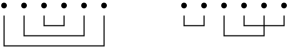
Figure 1: Two pairings of $[6]=\{1,2,3,4,5,6\}$. The first (totally-nested) pairing is noncrossing, while the second is not.

It will be convenient to allow for more general partitions in the sequel. A partition of $[n]$ is (as the name suggests) a collection of mutually disjoint nonempty subsets $B_{1},\ldots,B_{r}$ of $[n]$ such that $B_{1}\sqcup\cdots\sqcup B_{r}=[n]$. The subsets are called the blocks of the partition. By convention we order the blocks by their least elements; that is, $\min B_{i}<\min B_{j}$ iff $i<j$. The set of all partitions on $[n]$ is denoted $\mathscr{P}(n)$, and the subset of all pairings is $\mathscr{P}_{2}(n)$.

Definition 1.27.

Let $\pi\in\mathscr{P}(n)$ be a partition of $[n]$. We say $\pi$ has a crossing if there are two distinct blocks $B_{1},B_{2}$ in $\pi$ with elements $x_{1},y_{1}\in B_{1}$ and $x_{2},y_{2}\in B_{2}$ such that $x_{1}<x_{2}<y_{1}<y_{2}$. (This is demonstrated in Figure 1.)

If $\pi\in\mathscr{P}(n)$ has no crossings, it is said to be a noncrossing partition. The set of noncrossing partitions of $[n]$ is denoted $NC(n)$. The subset of noncrossing pairings is denoted $NC_{2}(n)$.

The reader is referred to NicaSpeicherBook for an extremely in-depth discussion of the algebraic and enumerative properties of the lattices $NC(n)$. For our purposes, we present only those structural features that will be needed in the analysis of Wigner integrals.

Definition 1.28.

Let $n_{1},\ldots,n_{r}$ be positive integers with $n=n_{1}+\cdots+n_{r}$. The set $[n]$ is then partitioned accordingly as $[n]=B_{1}\sqcup\cdots\sqcup B_{r}$ where $B_{1}=\{1,\ldots,n_{1}\}$, $B_{2}=\{n_{1}+1,\ldots,n_{1}+n_{2}\}$, and so forth through $B_{r}=\{n_{1}+\cdots+n_{r-1}+1,\ldots,n_{1}+\cdots+n_{r}\}$. Denote this partition as $n_{1}\otimes\cdots\otimes n_{r}$.

Say that a pairing $\pi\in\mathscr{P}_{2}(n)$ respects $n_{1}\otimes\cdots\otimes n_{r}$ if no block of $\pi$ contains more than one element from any given block of $n_{1}\otimes\cdots\otimes n_{r}$. (This is demonstrated in Figure 2.) The set of such respectful pairings is denoted $\mathscr{P}_{2}(n_{1}\otimes\cdots\otimes n_{r})$. The set of noncrossing pairings that respect $n_{1}\otimes\cdots\otimes n_{r}$ is denoted $NC_{2}(n_{1}\otimes\cdots\otimes n_{r})$.

Partitions $n_{1}\otimes\cdots\otimes n_{r}$ as described in Definition 1.28 are called interval partitions, since all of their blocks are intervals. Figure 2 gives some examples of respectful pairings.

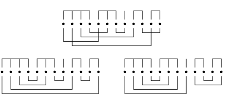
Figure 2: The partition $4\otimes 3\otimes 1\otimes 2\otimes 2$ is drawn above the dots; below are three pairings that respect it. The two bottom pairings are in $NC_{2}(4\otimes 3\otimes 1\otimes 2\otimes 2)$.

Remark 1.29.

The same definition of respectful makes perfect sense for more general partitions, but we will not have occasion to use it for anything but pairings. However, see Remark 1.32.

Remark 1.30.

Consider the partition $n_{1}\otimes\cdot\cdot\cdot\otimes n_{r}=\{B_{1},\ldots,B_{r}\}$, as well as a pairing $\pi\in\mathscr{P}_{2}(n)$, where $n=n_{1}+\cdots+n_{r}$. In the classical literature about Gaussian subordinated random fields (cf. PecTaqbook , Chapter 4, and the references therein) the pair $(n_{1}\otimes\cdot\cdot\cdot\otimes n_{r},\pi)$ is represented graphically as follows: (i) draw the blocks $B_{1},\ldots,B_{r}$ as superposed rows of dots (the $i$th row containing exactly $n_{i}$ dots, $i=1,\ldots,r$), and (ii) join two dots with an edge if and only if the corresponding two elements constitute a block of $\pi$. The graph thus obtained is customarily called a Gaussian diagram. Moreover, if $\pi$ respects $n_{1}\otimes\cdots\otimes n_{r}$ according to Definition 1.28, then the Gaussian diagram is said to be nonflat, in the sense that all its edges join different horizontal lines, and therefore are not flat, that is, not horizontal. The noncrossing condition is difficult to discern from the Gaussian diagram representation, which is why we do not use it here; therefore the nonflat terminology is less meaningful for us, and we prefer the intuitive notation from Definition 1.28.

One more property of pairings will be necessary in the proceeding analysis.

Definition 1.31.

Let $n_{1},\ldots,n_{r}$ be positive integers, and let $\pi\in\mathscr{P}_{2}(n_{1}\otimes\cdots\otimes n_{r})$. Let $B_{1}$, $B_{2}$ be two blocks in $n_{1}\otimes\cdots\otimes n_{r}$. Say that $\pi$ links $B_{1}$ and $B_{2}$ if there is a block $\{i,j\}\in\pi$ such that $i\in B_{1}$ and $j\in B_{2}$.

Define a graph $C_{\pi}$ whose vertices are the blocks of $n_{1}\otimes\cdots\otimes n_{r}$; $C_{\pi}$ has an edge between $B_{1}$ and $B_{2}$ iff $\pi$ links $B_{1}$ and $B_{2}$. Say that $\pi$ is connected with respect to $n_{1}\otimes\cdots\otimes n_{r}$ (or that $\pi$ connects the blocks of $n_{1}\otimes\cdots\otimes n_{r}$) if the graph $C_{\pi}$ is connected.

Denote by $NC_{2}^{c}(n_{1}\otimes\cdots\otimes n_{r})$ the set of noncrossing pairings that both respect and connect $n_{1}\otimes\cdots\otimes n_{r}$.

For example, the second partition in Figure 2 is in $NC_{2}^{c}(4\otimes 3\otimes 1\otimes 2\otimes 2)$, while the third is not. The interested reader may like to check that $NC_{2}(4\otimes 3\otimes 1\otimes 2\otimes 2)$ has $5$ elements, and all are connected except the third example in Figure 2.

Remark 1.32.

For a positive integer $n$, the set $NC(n)$ of noncrossing partitions on $[n]$ is a lattice whose partial order is given by reverse refinement. The top element $1_{n}$ is the partition $\{\{1,\ldots,n\}\}$ containing only one block; the bottom element $0_{n}$ is $\{\{1\},\ldots,\{n\}\}$ consisting of $n$ singletons. The conditions of Definitions 1.28 and 1.31 can be described elegantly in terms of the lattice operations meet $\wedge$ (i.e., inf) and join $\vee$ (i.e., sup). If $n=n_{1}+\cdots+n_{r}$, then $\pi\in NC_{2}(n)$ respects $n_{1}\otimes\cdots\otimes n_{r}$ if and only if $\pi\wedge(n_{1}\otimes\cdots\otimes n_{r})=0_{n}$; $\pi$ connects the blocks of $n_{1}\otimes\cdots\otimes n_{r}$ if and only if $\pi\vee(n_{1}\otimes\cdots\otimes n_{r})=1_{n}$.

Remark 1.33.

Given $n_{1},\ldots,n_{r}$ and a respectful noncrossing pairing $\pi\in NC_{2}(n_{1}\otimes\cdots\otimes n_{r})$, there is a unique decomposition of the full index set $[n]$, where $n=n_{1}+\cdots+n_{r}$, into subsets $D_{1},\ldots,D_{m}$ of the blocks of $n_{1}\otimes\cdots\otimes n_{r}$, such that the restriction of $\pi$ to each $D_{i}$ connects the blocks of $D_{i}$. These $D_{i}$ are the vertices of the graph $C_{\pi}$ grouped according to connected components of the graph. For example, in the third pairing in Figure 2, the decomposition has two components, $D_{1}=4\otimes 3\otimes 1$ and $D_{2}=2\otimes 2$. To be clear, this notation is slightly misleading since the $2\otimes 2$ in this case represents indices $\{9,10\},\{11,12\}$, not $\{1,2\},\{3,4\}$; we will be a little sloppy about this to make the following much more readable.

There is a close connection between respectful noncrossing pairings and expectations of products of Wigner integrals. To see this, we first introduce an action of pairings on functions.

Definition 1.34.

Let $n$ be an even integer, and let $\pi\in\mathscr{P}_{2}(n)$. Let $f\dvtx{\mathbb{R}}_{+}^{n}\to{\mathbb{C}}$ be measurable. The pairing integral of $f$ with respect to $\pi$, denoted $\int_{\pi}f$, is defined (when it exists) to be the constant

$$\int_{\pi}f=\int f(t_{1},\ldots,t_{n})\prod_{\{i,j\}\in\pi}\delta(t_{i}-t_{j})\,dt_{1}\cdots\,dt_{n}.\vspace*{-2pt}$$

For example, given the second pairing $\pi=\{\{1,2\},\{3,5\},\{4,6\}\}$ in Figure 1,

$$\int_{\pi}f=\int_{{\mathbb{R}}_{+}^{3}}f(r,r,s,t,s,t)\,dr\,ds\,dt.\vspace*{-2pt}$$

Remark 1.35.

The operation $\int_{\pi}$ is not well defined on $L^{2}({\mathbb{R}}_{+}^{n})$; for example, if $n=2$ and $\pi=\{\{1,2\}\}$, then $\int_{\pi}f$ is finite if and only if $f$ is the kernel of a trace class Hilbert–Schmidt operator on $L^{2}({\mathbb{R}}_{+})$. However, it is easy to see that $\int_{\pi}f$ is well-defined whenever $f$ is a tensor product of functions, and $\pi$ respects the interval partition induced by this tensor product (cf. Lemma 2.1). (This is one of the reasons why one should interpret multiple stochastic integrals as integrals on product spaces without diagonals, since integrals on diagonals are in general not defined.) This is precisely the case we will deal with in all of the following.

Note that a contraction $f\stackrel{{\scriptstyle p}}{{\frown}}g$ can be interpreted in terms of a pairing integral, using a partial pairing, that is, one that pairs only a subset of the indices. If $f\in L^{2}({\mathbb{R}}_{+}^{n})$ and $g\in L^{2}({\mathbb{R}}_{+}^{m})$, and $p\leq\min\{n,m\}$ is a natural number, then

$$f\stackrel{{\scriptstyle p}}{{\frown}}g=\int_{\tau_{p}}f\otimes g,$$

where $\tau_{p}$ is the partial pairing $\{\{n,n+1\},\{n-1,n+2\},\ldots,\{n-p+1,n+p\}\}$ of $[n+m]$.

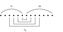
Figure 3: A partial pairing $\tau_{p}$ of $[n+m]$ corresponding to a $p$-contraction; here $n=6$, $m=7$, and $p=4$.

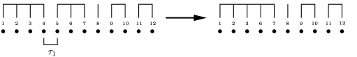
Figure 4: The partial pairing $\tau_{1}$ acts on the left on $4\otimes 3\otimes 1\otimes 2\otimes 2$, joining the first two blocks and deleting the middle indices, to produce the partition $5\otimes 1\otimes 2\otimes 2$. The indices are labeled to make the action clearer.

The partial contraction pairings $\tau_{p}$ provide a useful decomposition of the set of all respectful noncrossing pairings, in the following sense. Let $n_{1},\ldots,n_{r}$ be positive integers. If $p\leq\min\{n_{1},n_{2}\}$, the partial pairing $\tau_{p}$ acts (on the left) on the partition $n_{1}\otimes n_{2}\otimes n_{3}\otimes\cdots\otimes n_{r}$ to produce the partition $(n_{1}+n_{2}-2p)\otimes n_{3}\otimes\cdots\otimes n_{r}$. That is, $\tau_{p}$ joins the first two blocks of $n_{1}\otimes\cdots\otimes n_{r}$ and deletes the paired indices to produce a new interval partition. This is demonstrated in Figure 4.

Considered as such a function, we may then compose partial contraction pairings. For example, following Figure 4, we may act again with $\tau_{1}$ on $5\otimes 1\otimes 2\otimes 2$ to yield $4\otimes 2\otimes 2$; then with $\tau_{2}$ to get $2\otimes 2$; and finally $\tau_{2}$ maps this partition to the empty partition. Stringing these together gives a respectful pairing of the original interval partition, which we denote $\tau_{2}\circ\tau_{2}\circ\tau_{1}\circ\tau_{1}$. Figure 5 displays this composition.

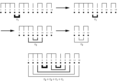
Figure 5: The composition $\tau_{2}\circ\tau_{2}\circ\tau_{1}\circ\tau_{1}$ produces a noncrossing pairing that respects $4\otimes 3\otimes 1\otimes 2\otimes 2$.

To be clear: we start from the left and then do the partial pairing $\tau_{p}$ between the first and second block; after this application, the (rest of the) first and second blocks are treated as a single block. This is still the case if $p=0$; here there are no paired indices, but the action of $\tau_{0}$ records the fact that, for further discussion, the first two blocks are now connected. An example is given in Figure 6 below, where the action of $\tau_{0}$ is graphically represented by a dashed line.

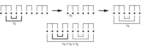
Figure 6: The pairing $\pi=\{\{1,10\},\{2,5\},\{3,4\},\{6,9\},\{7,8\}\}$ respects the interval partition $3\otimes 2\otimes 2\otimes 3$. Its decomposition is given by $\pi=\tau_{3}\circ\tau_{0}\circ\tau_{2}$.

With this convention, further $\tau_{p}$ may act only on the first two blocks, which results in a unique decomposition of any respectful pairing into partial contractions, as the next lemma makes clear.

Lemma 1.36.

Let $n_{1},\ldots,n_{r}$ be positive integers, and let $\pi\in NC_{2}(n_{1}\otimes\cdots\otimes n_{r})$. There is a unique sequence of partial contractions $\tau_{p_{1}},\ldots,\tau_{p_{r-1}}$ such that $\pi=\tau_{p_{r-1}}\circ\cdots\circ\tau_{p_{1}}$.

Any noncrossing pairing must contain an interval $\{i,i+1\}$; cf. NicaSpeicherBook , Remark 9.2(2). Hence, since $\pi$ respects $n_{1}\otimes\cdots\otimes n_{r}=\{B_{1},\ldots,B_{r}\}$, there must be two adjacent blocks linked by $\pi$. Let $j\in[k]$ be the smallest index for which $B_{j},B_{j+1}$ are connected by $\pi$; hence all of the blocks $B_{1},\ldots,B_{j}$ pair among the blocks $B_{j+1},\ldots,B_{r}$. Note that any partition that satisfies this constraint and also respects the coarser interval partition $(n_{1}+\cdots+n_{j})\otimes n_{j+1}\otimes\cdots\otimes n_{r}$ is automatically in $NC_{2}(n_{1}\otimes\cdots\otimes n_{r})$. In other words, we can begin by decomposing $\pi=\pi^{\prime}\circ(\tau_{0})^{j-1}$, where $\pi^{\prime}\in NC_{2}((n_{1}+\cdots+n_{j})\otimes n_{j+1}\otimes\cdots\otimes n_{r})$ links the first and second blocks of this interval partition. By construction, this $j$ is unique.

Let $n_{0}=n_{1}+\cdots+n_{j}$, so $\pi^{\prime}$ links $\{1,\ldots,n_{0}\}$ with $\{n_{0}+1,\ldots,n_{0}+n_{j+1}\}$. It follows that $\{n_{0},n_{0}+1\}\in\pi^{\prime}$: for if $n_{0}$ pairs with some element $n_{0}+i$ with $i\geq 2$, then $n_{0}+1,\ldots,n_{0}+i-1$ cannot pair anywhere without introducing crossings. Following these lines, an easy induction shows that there is some $p\in[\min\{n_{0},n_{j+1}\}]$ such that the pairs $\{n_{0},n_{0}+1\},\{n_{0}-1,n_{0}+2\},\ldots,\{n_{0}-p+1,n_{0}+p\}$ are in $\pi^{\prime}$, while all indices $1,\ldots,n_{0}-p$ and $n_{0}+p+1,\ldots,n_{0}+n_{j+1}$ pair outside $[n_{0}+n_{j+1}]$. In other words, $\pi^{\prime}=\pi^{\prime\prime}\circ\tau_{p}$ for some noncrossing pairing $\pi^{\prime\prime}$ that respects $(n_{0}-p)\otimes(n_{j+1}-p)\otimes n_{3}\otimes\cdots\otimes n_{r}$. What’s more, since $p$ was chosen maximally so that there are no further pairings in the blocks $(n_{0}-p)\otimes(n_{j+1}-p)$, these two may be treated as a single block, and $\pi^{\prime\prime}$ is only constrained to be in $NC_{2}(n_{0}+n_{j+1}-2p,n_{3},\ldots,n_{r})$. Since $p>0$, the lemma now follows by a finite induction; uniqueness results from the left-most choice of $j$ and maximal choice of $p$ at each stage.

By carefully tracking the proof of Lemma 1.36, we can give a complete description of the class of respectful pairings in terms of their decompositions.

Lemma 1.37.

Let $n_{1},\ldots,n_{r}$ be positive integers. The class $NC_{2}(n_{1}\otimes\cdots\otimes n_{r})$ is equal to the set of compositions $\tau_{p_{r-1}}\circ\cdots\circ\tau_{p_{1}}$ where $(p_{1},\ldots,p_{r-1})$ satisfy the inequalities

$$0 \leq p_{1}\leq\min\{n_{2},n_{1}\},$$

$$0 \leq p_{k}\leq\min\{n_{k+1},n_{1}+\cdots+n_{k}-2p_{1}-\cdots-2p_{k-1}\},$$ (8)

$$\eqntext{1<k<r-1,2(p_{1}+\cdots+p_{r-1})=n_{1}+\cdots+n_{r}.}$$ (9)

Inequalities (1.37) in Lemma 1.37 successively guarantee that the partial contractions $\tau_{p_{k}}$ in the decomposition of $\pi$ only contract elements from within two adjacent blocks; the final equality is to guarantee that all indices are paired in the end. Since every respectful pairing has a contraction decomposition, and each contraction decomposition satisfying inequalities (1.37) is respectful (a fact which follows from an easy induction), these inequalities define $NC_{2}(n_{1}\otimes\cdots\otimes n_{r})$. This completely combinatorial description would be the starting point for an enumeration of the class of respectful pairings; however, even in the case $n_{1}=\cdots=n_{r}$, the enumeration appears to be extremely difficult.

We conclude this section with a proposition that demonstrates the efficacy of pairing integrals and noncrossing pairings in the analysis of Wigner integrals.

Proposition 1.38

Let $n_{1},\ldots,n_{r}$ be positive integers, and suppose $f_{1},\ldots,\allowbreak f_{r}$ are functions with $f_{i}\in L^{2}({\mathbb{R}}_{+}^{n_{i}})$ for $1\leq i\leq r$. The expectation $\varphi$ of the product of Wigner integrals $I_{n_{1}}^{S}(f_{1})\cdots I_{n_{r}}^{S}(f_{r})$ is given by

$$\varphi[I_{n_{1}}^{S}(f_{1})\cdots I_{n_{r}}^{S}(f_{r})]=\sum_{\pi\in NC_{2}(n_{1}\otimes\cdots\otimes n_{r})}\int_{\pi}f_{1}\otimes\cdots\otimes f_{r}.$$ (10)

Remark 1.39.

This result has been used in the literature (e.g., to prove BianeSpeicher , Theorem 5.3.4), but it appears to have a folklore status in that a proof has not been written down. The following proof is an easy application of Proposition 1.25, together with Lemma 1.37.

By iterating equation (7), we arrive at the following unwieldy expression. (For readability, we have hidden the explicit dependence of the Wigner integral $I^{S}_{n}$ on the number of variables $n$ in its argument.)

$$I^{S}(f_{1})\cdots I^{S}(f_{r})=\sum_{p_{r-1}}\cdots\sum_{p_{1}}I^{S}\bigl{(}\bigl{(}\cdots\bigl{(}(f_{1}\stackrel{{\scriptstyle p_{1}}}{{\frown}}f_{2})\stackrel{{\scriptstyle p_{2}}}{{\frown}}f_{3}\bigr{)}\cdots\bigr{)}\stackrel{{\scriptstyle p_{r-1}}}{{\frown}}f_{r}\bigr{)},$$ (11)

where $p_{1},\ldots,p_{r-1}$ range over the set specified by the first two inequalities in equation (1.37). (This is the range of the $p_{k}$ for the same reason that those inequalities specify the range of the $p_{k}$ for contraction decompositions: the first two inequalities in (1.37) merely guarantee that contractions are performed, successively, only between two adjacent blocks of $n_{1}\otimes\cdots\otimes n_{r}$.) Note: following Remark 1.22, the order the contractions are performed in equation (11) is important.

Taking expectation in equation (11), note that most terms have $\varphi=0$ since any nontrivial stochastic integral is centred (as it is orthogonal to constants in the $0$th order of chaos). Hence, the only terms that contribute to the sum are those for which the iterated contractions pair all indices of the functions; that is, the sum is over those $p_{1},\ldots,p_{r-1}$ for which $2(p_{1}+\cdots+p_{r-1})=n_{1}+\cdots+n_{r}$, so that the stochastic integral $I^{S}$ in the sum is $I^{S}_{0}$. Since such a trivial stochastic integral is just the identity on the constant function inside, this shows that

$$\varphi[I^{S}(f_{1})\cdots I^{S}(f_{r})]=\sum_{p_{r-1}}\cdots\sum_{p_{1}}\bigl{(}\bigl{(}\cdots\bigl{(}(f_{1}\stackrel{{\scriptstyle p_{1}}}{{\frown}}f_{2})\stackrel{{\scriptstyle p_{2}}}{{\frown}}f_{3}\bigr{)}\cdots\bigr{)}\stackrel{{\scriptstyle p_{r-1}}}{{\frown}}f_{r}\bigr{)},$$

where the sum is over those $p_{1},\ldots,p_{r-1}$ satisfying the same inequalities mentioned above, along with the condition $2(p_{1}+\cdots+p_{r-1})=n_{1}+\cdots+n_{r}$; that is, the $p_{k}$ satisfy inequalities (1.37). Each such iterated contraction integral corresponds to a pairing integral of $f_{1}\otimes\cdots\otimes f_{r}$ in the obvious fashion,

$$\bigl{(}\bigl{(}\cdots\bigl{(}(f_{1}\stackrel{{\scriptstyle p_{1}}}{{\frown}}f_{2})\stackrel{{\scriptstyle p_{2}}}{{\frown}}f_{3}\bigr{)}\cdots\bigr{)}\stackrel{{\scriptstyle p_{r-1}}}{{\frown}}f_{r}\bigr{)}=\int_{\tau_{p_{r-1}}\circ\cdots\circ\tau_{p_{1}}}f_{1}\otimes\cdots\otimes f_{r}.$$

Lemma 1.37 therefore completes the proof.

Remark 1.40.

Another proof of Proposition 1.38 can be achieved using a random matrix approximation to the free Brownian motion, as discussed in Section 1.2. The starting point is the classical counterpoint to Proposition 1.38 Janson , Theorem 7.33, which states that the expectation of a product of Wiener integrals is a similar sum of pairing integrals over respectful (i.e., nonflat) pairings, but in this case crossing pairings must also be included. Modifying this formula for matrix-valued Brownian motion, and controlling the leading terms in the limit as matrix size tends to infinity using the so-called “genus expansion,” leads to equation (10). The (quite involved) details are left to the interested reader.

2 Central limit theorems

We begin by proving Theorem 1.6, which we restate here for convenience.

Let $n$ be a natural number, and let $(f_{k})_{k\in{\mathbb{N}}}$ be a sequence of functions in $L^{2}({\mathbb{R}}_{+}^{n})$, each with $\|f_{k}\|_{L^{2}({\mathbb{R}}_{+}^{n})}=1$. The following statements are equivalent: [(2)]

The fourth absolute moments of the stochastic integrals $I^{S}_{n}(f_{k})$ converge to $2$.

$$\lim_{k\to\infty}\varphi(|I^{S}_{n}(f_{k})|^{4})=2.$$

All nontrivial contractions of $f_{k}$ converge to $0$. For each $p=1,2,\ldots,\allowbreak n-1$,

$$\lim_{k\to\infty}f_{k}\stackrel{{\scriptstyle p}}{{\frown}}f_{k}^{\ast}=0\qquad\mbox{in }L^{2}({\mathbb{R}}_{+}^{2n-2p}).\vspace*{-2pt}$$

The expression $|I^{S}_{n}(f_{k})|^{4}$ is short-hand for $[I_{n}^{S}(f_{k})\cdot I_{n}^{S}(f_{k})^{\ast}]^{2}$. Since [according to equation (1.3)] $I_{n}^{S}(f_{k})^{\ast}=I_{n}^{S}(f_{k}^{\ast})$, this is a product of Wigner integrals, to which we will apply Proposition 1.25. First,

$$I_{n}^{S}(f_{k})\cdot I_{n}^{S}(f_{k}^{\ast})=\sum_{p=0}^{n}I_{2n-2p}^{S}(f_{k}\stackrel{{\scriptstyle p}}{{\frown}}f_{k}^{\ast}).$$ (12)

The Wigner integrals on the right-hand side of equation (12) are in different orders of chaos, and hence are orthogonal (with respect to the $\varphi$-inner product). Thus, we can expand

$$\varphi(|I_{n}^{S}(f_{k})|^{4}) = \varphi\bigl{[}\bigl{(}I_{n}^{S}(f_{k})\cdot I_{n}^{S}(f_{k}^{\ast})\bigr{)}^{2}\bigr{]}$$

$$= \langle I_{n}^{S}(f_{k})\cdot I_{n}^{S}(f_{k}^{\ast}),I_{n}^{S}(f_{k})\cdot I_{n}^{S}(f_{k}^{\ast})\rangle_{\varphi}$$

$$= \sum_{p=0}^{n}\langle I_{2n-2p}^{S}(f_{k}\stackrel{{\scriptstyle p}}{{\frown}}f_{k}^{\ast}),I_{2n-2p}^{S}(f_{k}\stackrel{{\scriptstyle p}}{{\frown}}f_{k}^{\ast})\rangle_{\varphi},$$

where in the second equality we have used the fact that $I_{n}^{S}(f_{k})\cdot I_{n}^{S}(f_{k}^{\ast})$ is self adjoint. Now employing the Wigner isometry [equation (5)], this yields

$$\varphi(|I_{n}^{S}(f_{k})|^{4})=\sum_{p=0}^{n}\langle f_{k}\stackrel{{\scriptstyle p}}{{\frown}}f_{k}^{\ast},f_{k}\stackrel{{\scriptstyle p}}{{\frown}}f_{k}^{\ast}\rangle_{L^{2}({\mathbb{R}}_{+}^{2n-2p})}.$$ (13)

Consider first the two boundary terms in the sum in equation (13). When $p=n$, we have

$$f_{k}\stackrel{{\scriptstyle n}}{{\frown}}f_{k}^{\ast}=\langle f_{k},f_{k}\rangle_{L^{2}({\mathbb{R}}_{+}^{n})}=1,$$

according to Lemma 1.24(2) and the assumption that $f_{k}$ is normalized in $L^{2}$. On the other hand, when $p=0$, the contraction $f_{k}\stackrel{{\scriptstyle 0}}{{\frown}}f_{k}$ is just the tensor product $f\otimes f^{\ast}$, and we have

$$\langle f_{k}\otimes f_{k}^{\ast},f_{k}\otimes f_{k}^{\ast}\rangle_{L^{2}({\mathbb{R}}_{+}^{2n})}=\langle f_{k},f_{k}\rangle_{L^{2}({\mathbb{R}}_{+}^{n})}\langle f_{k}^{\ast},f_{k}^{\ast}\rangle_{L^{2}({\mathbb{R}}_{+}^{n})}=1.$$

(Both terms in the product are equal to $\|f_{k}\|_{L^{2}}^{2}=1$, following Definition 1.19 of $f_{k}^{\ast}$.) Equation (13) can therefore be rewritten as

$$\varphi(|I_{n}^{S}(f_{k})|^{4})=2+\sum_{p=1}^{n-1}\|f_{k}\stackrel{{\scriptstyle p}}{{\frown}}f_{k}^{\ast}\|_{L^{2}({\mathbb{R}}_{+}^{2n-2p})}^{2}.$$ (14)

Thus, the statement that the limit of $\varphi(|I_{n}^{S}(f_{k})|^{4})$ equals $2$ is equivalent to the statement that the limit of the sum on the right-hand side of equation (14) is $0$. This is a sum of nonnegative terms, and so each of the terms must have limit $0$. This completes the proof.

Corollary 1.7 now follows quite easily.

Let $n\geq 2$ be an integer, and consider a nonzero mirror symmetric function $f\in L^{2}({\mathbb{R}}_{+}^{n})$. Then the Wigner integral $I_{n}^{S}(f)$ satisfies $\varphi[I_{n}^{S}(f)^{4}]>2\varphi[I_{n}^{S}(f)^{2}]^{2}$. In particular, the distribution of the Wigner integral $I^{S}_{n}(f)$ cannot be semicircular.

By rescaling, we may assume that $\|f\|_{L^{2}({\mathbb{R}}_{+}^{n})}=1$; in this case, equation (14) shows that $\varphi[I_{n}^{S}(f)^{4}]\geq 2\varphi[I_{n}^{S}(f)^{2}]^{2}$. To achieve a contradiction, we assume that $\varphi[I_{n}^{S}(f)^{4}]=2\varphi[I_{n}^{S}(f)^{2}]^{2}=2$ [which would be the case if $I_{n}^{S}(f)$ were semicircular]. Then the constant sequence $f_{k}=f$ for all $k$ satisfies condition (1) of Theorem 1.6; hence, for $1\leq p\leq n-1$,

$$f\stackrel{{\scriptstyle p}}{{\frown}}f^{\ast}=\lim_{k\to\infty}f_{k}\stackrel{{\scriptstyle p}}{{\frown}}f_{k}^{\ast}=0\qquad\mbox{in }L^{2}({\mathbb{R}}_{+}^{2n-2p}).$$

Take, for example, $p=n-1$. Let $g\in L^{2}({\mathbb{R}}_{+})$, so that $g\otimes g^{\ast}\in L^{2}({\mathbb{R}}_{+}^{2})$. Then we may calculate the inner product

$$\langle f\stackrel{{\scriptstyle n-1}}{{\frown}}f^{\ast},g\otimes g^{\ast}\rangle_{L^{2}({\mathbb{R}}_{+}^{2})}$$

$$\qquad=\int[f\stackrel{{\scriptstyle n-1}}{{\frown}}f^{\ast}](s,t)\overline{[g\otimes g^{\ast}](s,t)}\,ds\,dt$$

$$\qquad=\int\biggl{(}\int f(s,s_{2},\ldots,s_{n})f^{\ast}(s_{n},\ldots,s_{2},t)\,ds_{2}\cdots\,ds_{n}\biggr{)}\overline{g(s)}g(t)\,ds\,dt$$

$$\qquad=\int g^{\ast}(s)f(s,s_{2},\ldots,s_{n})\cdot\overline{g^{\ast}(t)f(t,s_{2},\ldots,s_{n})}\,ds\,dt\,ds_{2}\cdots\,ds_{n}$$

$$\qquad=\|g^{\ast}\stackrel{{\scriptstyle 1}}{{\frown}}f\|_{L^{2}({\mathbb{R}}_{+}^{n-1})}^{2}.$$

By assumption, $f\stackrel{{\scriptstyle n-1}}{{\frown}}f^{\ast}=0$, and so we have $g^{\ast}\stackrel{{\scriptstyle 1}}{{\frown}}f=0$ for all $g\in L^{2}({\mathbb{R}}_{+})$. That is, for almost all $s_{2},\ldots,s_{n}\in{\mathbb{R}}_{+}$,

$$\int_{0}^{\infty}\overline{g(s)}f(s,s_{2},\ldots,s_{n})\,ds=0.$$

For fixed $s_{2},\ldots,s_{n}$ for which this holds, taking $g$ to be the function $g(s)=f(s,s_{2},\ldots,s_{n})$ yields that $f(s,s_{2},\ldots,s_{n})=0$ for almost all $s$. Hence, $f=0$ almost surely. This contradicts the normalization $\|f\|_{L^{2}({\mathbb{R}}_{+}^{n})}=1$.

We now proceed towards the proof of Theorem 1.3. First, we state a technical result that will be of use.

Lemma 2.1.

Let $n_{1},\ldots,n_{r}$ be positive integers, and let $f_{i}\in L^{2}({\mathbb{R}}_{+}^{n_{i}})$ for $1\leq i\leq r$. Let $\pi$ be a pairing in $\mathscr{P}_{2}(n_{1}\otimes\cdots\otimes n_{r})$. Then

$$\biggl{|}\int_{\pi}f_{1}\otimes\cdots\otimes f_{r}\biggr{|}\leq\|f_{1}\|_{L^{2}({\mathbb{R}}_{+}^{n_{1}})}\cdots\|f_{r}\|_{L^{2}({\mathbb{R}}_{+}^{n_{r}})}.$$

This follows by iterated application of the Cauchy–Schwarz inequality along the pairs in $\pi$. It is proved as Janson , Lemma 7.31.

The following proposition shows that contractions control all important pairing integrals.

Proposition 2.2

Let $n$ be a positive integer. Consider a sequence $(f_{k})_{k\in{\mathbb{N}}}$ with $f_{k}\in L^{2}({\mathbb{R}}_{+}^{n})$ for all $k$, such that: [(3)]

$f_{k}=f_{k}^{\ast}$ for all $k$;

there is a constant $M>0$ such that $\|f_{k}\|_{L^{2}({\mathbb{R}}_{+}^{n})}\leq M$ for all $k$;

for each $p=1,2,\ldots,n-1$,

$$\lim_{k\to\infty}f_{k}\stackrel{{\scriptstyle p}}{{\frown}}f_{k}^{\ast}=0\qquad\mbox{in }L^{2}({\mathbb{R}}_{+}^{2n-2p}).$$

Let $r\geq 3$, and let $\pi$ be a connected noncrossing pairing that respects $n^{\otimes r}$: $\pi\in NC_{2}^{c}(n^{\otimes r})$; cf. Definitions 1.28 and 1.31. Then

$$\lim_{k\to\infty}\int_{\pi}f_{k}^{\otimes r}=0.$$

Begin by decomposing $\pi=\tau_{p_{r-1}}\circ\cdots\circ\tau_{p_{1}}$ following Lemma 1.36. There must be some nonzero $p_{i}$; to simplify notation, we assume that $p_{1}>0$. (Otherwise we may perform a cyclic rotation and relabel indices from the start.) Note also that, since $\pi$ connects the blocks of $n^{\otimes r}$ and $r>2$, it follows that $p_{1}<n$: else the first two blocks $\{1,\ldots,n\}$ and $\{n+1,\ldots,2n\}$ would form a connected component in the graph $C_{\pi}$ from Definition 1.31, so $C_{\pi}$ would not be connected. Set $\pi^{\prime}=\tau_{p_{k}}\circ\cdots\circ\tau_{p_{2}}$, so that $\pi=\pi^{\prime}\circ\tau_{p_{1}}$. Then (as in the proof of Proposition 1.38) it follows that

$$\int_{\pi}f_{k}^{\otimes r}=\int_{\pi^{\prime}}(f_{k}\stackrel{{\scriptstyle p_{1}}}{{\frown}}f_{k})\otimes f_{k}^{\otimes(r-2)}.$$ (15)

To make this clear, an example is given in Figure 7, with the corresponding iterations of the integral in equation (2).

$$\int_{\pi}f^{\otimes 4} = \int_{{\mathbb{R}}_{+}^{6}}f(t_{1},t_{2},t_{3})f(t_{3},t_{2},t_{4})f(t_{4},t_{5},t_{6})f(t_{6},t_{5},t_{1})\,dt_{1}\,dt_{2}\,dt_{3}\,dt_{4}\,dt_{5}\,dt_{6}$$

$$= \int_{{\mathbb{R}}_{+}^{4}}(f\stackrel{{\scriptstyle 2}}{{\frown}}f)(t_{1},t_{4})f(t_{4},t_{5},t_{6})f(t_{6},t_{5},t_{1})\,dt_{1}\,dt_{4}\,dt_{5}\,dt_{6}$$

$$= \int_{\pi^{\prime}}(f\stackrel{{\scriptstyle 2}}{{\frown}}f)\otimes f^{\otimes 2}.$$

Employing Lemma 2.1, we therefore have

$$\biggl{|}\int_{\pi}f_{k}^{\otimes r}\biggr{|} = \biggl{|}\int_{\pi^{\prime}}(f_{k}\stackrel{{\scriptstyle p_{1}}}{{\frown}}f_{k})\otimes f_{k}^{\otimes(r-2)}\biggr{|}$$

$$\leq \|f_{k}\stackrel{{\scriptstyle p_{1}}}{{\frown}}f_{k}\|_{L^{2}({\mathbb{R}}_{+}^{2n-2p})}\cdot\|f_{k}\|_{L^{2}({\mathbb{R}}_{+}^{n})}^{r-2}$$

$$\leq \|f_{k}\stackrel{{\scriptstyle p_{1}}}{{\frown}}f_{k}\|_{L^{2}({\mathbb{R}}_{+}^{2n-2p})}\cdot M^{r-2},$$

using assumption (2) in the proposition. But from assumptions (1) and (3), $\|f_{k}\stackrel{{\scriptstyle p_{1}}}{{\frown}}f_{k}\|_{L^{2}({\mathbb{R}}_{+}^{2n-2p})}\to 0$. The result follows.

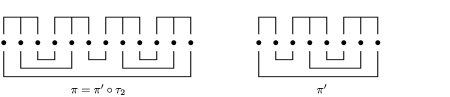
Figure 7: A pairing $\pi\in NC_{2}^{c}(3^{\otimes 4})$, with the first step in its contraction decomposition (per Lemma 1.36).

We can now prove the main theorem of the paper, Theorem 1.3, which we restate here for convenience.

Let $n\geq 2$ be an integer, and let $(f_{k})_{k\in{\mathbb{N}}}$ be a sequence of mirror symmetric functions in $L^{2}({\mathbb{R}}_{+}^{n})$, each with $\|f_{k}\|_{L^{2}({\mathbb{R}}_{+}^{n})}=1$. The following statements are equivalent: [(2)]

The fourth moments of the stochastic integrals $I^{S}_{n}(f_{k})$ converge to $2$.

$$\lim_{k\to\infty}\varphi(I^{S}_{n}(f_{k})^{4})=2.$$

The random variables $I^{S}_{n}(f_{k})$ converge in law to the standard semicircular distribution $S(0,1)$ as $k\to\infty$.

As pointed out in Remark 1.5, the implication (2)${}\Longrightarrow{}$(1) is essentially elementary: we need only demonstrate uniform tail estimates. In fact, the laws $\mu_{k}$ of $I^{S}_{n}(f_{k})$ are all uniformly compactly-supported: by BianeSpeicher , Theorem 5.3.4 (which is a version of the Haagerup inequality, cf. Haagerup ), any Wigner integral satisfies

$$\|I_{n}^{S}(f)\|\leq(n+1)\|f\|_{L^{2}({\mathbb{R}}_{+}^{n})}.$$

Since all the functions $f_{k}$ are normalized in $L^{2}$, it follows that $\operatorname{supp}\mu_{k}\subseteq[-n-1,n+1]$ for all $k$. Since the semicircle law is also supported in this interval, we may approximate the function $x\mapsto x^{4}$ by a $C_{c}({\mathbb{R}})$ function that agrees with it on all the supports, and hence convergence in distribution of $\mu_{k}$ to the semicircle law implies convergence of the fourth moments by definition.

We will use Proposition 2.2, together with Proposition 1.38, to prove the remarkable reverse implication. Since $S(0,1)$ is compactly supported, it is enough to verify that the moments of $I^{S}_{n}(f_{k})$ converge to the moments of $S(0,1)$, as described following equation (4). Since $I^{S}_{n}(f_{k})$ is orthogonal to the constant $1$ in the first order of chaos, $I^{S}_{n}(f_{k})$ is centred; the Wigner isometry of equation (5) yields that the second moment of $I^{S}_{n}(f_{k})$ is constantly $1$ due to normalization. Therefore, take $r\geq 3$. Proposition 1.38 yields that

$$\varphi[I^{S}_{n}(f_{k})^{r}]=\sum_{\pi\in NC_{2}(n^{\otimes r})}\int_{\pi}f_{k}^{\otimes r}.$$ (18)

Following Remark 1.33, any $\pi\in NC_{2}(n^{\otimes r})$ can be (uniquely) decomposed into a disjoint union of connected pairings $\pi=\pi_{1}\sqcup\cdots\sqcup\pi_{m}$ with $\pi_{i}\in NC_{2}^{c}(n^{\otimes r_{i}})$ for some $r_{i}$’s with $r_{1}+\cdots+r_{m}=r$. Since the decomposition respects the partition $n^{\otimes r}$, the pairing integrals decompose as products.

$$\int_{\pi}f_{k}^{\otimes r}=\prod_{i=1}^{m}\int_{\pi_{i}}f_{k}^{\otimes r_{i}}.$$ (19)

Assumption (1) in this theorem implies, by Theorem 1.6, that $f_{k}\stackrel{{\scriptstyle p}}{{\frown}}f_{k}^{\ast}\to 0$ in $L^{2}$ for each $p\in\{1,\ldots,n-1\}$. Therefore, from Proposition 2.2, it follows that for each of the decomposed connected pairings $\pi_{i}$ with $r_{i}\geq 3$, the corresponding pairing integral $\int_{\pi_{i}}f_{k}^{\otimes r_{i}}$ converges to $0$ in $L^{2}$. Since the number of factors $m$ in the product is bounded above by $r$ (which does not grow with $k$), this demonstrates that equation (18) really expresses the limiting $r$th moment as a sum over a small subset of $NC_{2}(n^{\otimes r})$. Let $NC_{2}^{2}(n^{\otimes r})$ denote the set of those respectful pairings $\pi$ such that, in the decomposition $\pi=\pi_{1}\sqcup\cdots\sqcup\pi_{m}$, each $r_{i}=2$, in other words, such that the connected components of the graph $C_{\pi}$ each have two vertices. Thus we have shown that

$$\lim_{k\to\infty}\varphi[I^{S}_{n}(f_{k})^{r}]=\sum_{\pi\in NC_{2}^{2}(n^{\otimes r})}\lim_{k\to\infty}\int_{\pi}f_{k}^{\otimes r}.$$ (20)

Note: if each $r_{i}=2$ and $r=r_{1}+\cdots+r_{m}$, then $r=2m$ is even. In other words, if $r$ is odd, then $NC_{2}^{2}(n^{\otimes r})$ is empty, and we have proved that all limiting odd moments of $I^{S}_{n}(f_{k})$ are $0$. If $r=2m$ is even, on the other hand, then the factors $\pi_{i}$ in the decomposition of $\pi$ can each be thought of as $\pi_{i}\in NC_{2}(n\otimes n)$. The reader may readily check that the only noncrossing pairing that respects $n\otimes n$ is the totally nested pairing $\pi_{i}=\{\{n,n+1\},\{n-1,n+2\},\ldots,\{1,2n\}\}$ in Figure 1. Thus, utilizing the mirror symmetry of $f_{k}$,

$$\int_{\pi_{i}}f_{k}\otimes f_{k}=\int_{\pi_{i}}f_{k}\otimes f_{k}^{\ast}=\|f_{k}\|_{L^{2}({\mathbb{R}}_{+}^{n})}^{2}=1.$$

Therefore, equation (20) reads

$$\lim_{k\to\infty}\varphi[I^{S}_{n}(f_{k})^{2m}]=\sum_{\pi\in NC_{2}^{2}(n^{\otimes 2m})}1=|NC_{2}^{2}(n^{\otimes 2m})|.$$ (21)

In each tensor factor of $n^{\otimes 2m}$, all edges of each pairing in $\pi$ act as one unit (since they pair in a uniform nested fashion as described above); this sets up a bijection $NC_{2}^{2}(n^{\otimes 2m})\cong NC_{2}(2m)$. The set of noncrossing pairings of $[2m]$ is well known to be enumerated by the Catalan number $C_{m}$ (cf. NicaSpeicherBook , Lemma 8.9), which is the $2m$th moment of $S(0,1)$; see the discussion following equation (4). This completes the proof.

Next we prove the Wigner–Wiener transfer principle, Theorem 1.8, restated below.

Let $n\geq 2$ be an integer, and let $(f_{k})_{k\in{\mathbb{N}}}$ be a sequence of fully symmetric functions in $L^{2}({\mathbb{R}}_{+}^{n})$. Let $\sigma>0$ be a finite constant. Then, as $k\to\infty$: [(2)]

${\mathbb{E}}[I^{W}_{n}(f_{k})^{2}]\to n!\sigma^{2}$ if and only if $\varphi[I^{S}_{n}(f_{k})^{2}]\to\sigma^{2}$;

if the asymptotic relations in (1) are verified, then $I^{W}_{n}(f_{k})$ converges in law to a normal random variable $N(0,n!\sigma^{2})$ if and only if $I^{S}_{n}(f_{k})$ converges in law to a semicircular random variable $S(0,\sigma^{2})$.

Point (1) is a simple consequence of the Wigner isometry of equation (5), stating that for fully symmetric $f\in L^{2}({\mathbb{R}}_{+}^{n})$, $\varphi[I^{S}_{n}(f)^{2}]=\|f\|_{2}^{2}$ (since $f$ is fully symmetric, $f=f^{\ast}$ in particular), together with the classical Wiener isometry which states that ${\mathbb{E}}[I^{W}_{n}(f)^{2}]=n!\|f\|_{2}^{2}$. For point (2), by renormalizing $f_{k}$ we may apply Theorems 1.3 and 1.6 to see that $I_{n}^{S}(f_{k})$ converges to $S(0,1)$ in law if and only if the contractions $f_{k}\stackrel{{\scriptstyle p}}{{\frown}}f_{k}^{\ast}=f_{k}\stackrel{{\scriptstyle p}}{{\frown}}f_{k}$ converge to $0$ in $L^{2}$ for $p=1,2,\ldots,n-1$. Since $f$ is fully symmetric, these nested contractions $f_{k}\stackrel{{\scriptstyle p}}{{\frown}}f_{k}$ are the same as the contractions $f\otimes_{p}f$ in nunugio (cf. Remark 1.23), and the main theorems in that paper show that these contractions tend to $0$ in $L^{2}$ if and only if the Wiener integrals $I^{W}_{n}(f_{k})$ converge in law to a normal random variable, with variance $n!$ due to our normalization. This completes the proof.

As an application, we prove a free analog of the Breuer–Major theorem for stationary vectors. This classical theorem can be stated as follows.

[(Breuer–Major theorem)] Let $(X_{k})_{k\in{\mathbb{Z}}}$ be a doubly-infinite sequence of (jointly Gaussian) standard normal random variables, and let $\rho(k)={\mathbb{E}}(X_{0}X_{k})$ denote the covariance function. Suppose there is an integer $n\geq 1$ such that $\sum_{k\in{\mathbb{Z}}}|\rho(k)|^{n}<\infty$. Let $H_{n}$ denote the $n$th Hermite polynomial,

$$H_{n}(x)=(-1)^{n}e^{x^{2}/2}\,\frac{d^{n}}{dx^{n}}e^{-x^{2}/2}.$$

($\{H_{n}\dvtx n\geq 0\}$ are the monic orthogonal polynomials associated to the law $N(0,1)$.) Then the sequence

$$V_{m}=\frac{1}{\sqrt{m}}\sum_{k=0}^{m-1}H_{n}(X_{k})\mathop{\longrightarrow}^{\mathrm{law}}N(0,n!\sigma^{2})\qquad\mbox{as }m\to\infty,$$

where $\sigma^{2}=\sum_{k\in{\mathbb{Z}}}\rho(k)^{n}$.

See, for example, the preprint NPP for extensions and quantitative improvements of this theorem. Note that the Hermite polynomial $H_{n}$ is related to Wiener integrals as follows: if $(W_{t})_{t\geq 0}$ is a standard Brownian motion, then $W_{1}$ is a $N(0,1)$ variable, and

$$H_{n}(W_{1})=I^{W}_{n}\bigl{(}{\mathbh 1}_{[0,1]^{n}}\bigr{)}.$$

(See, e.g., Kuo .) The function ${\mathbh 1}_{[0,1]^{n}}$ is fully symmetric. On the other hand, if $(S_{t})_{t\geq 0}$ is a free Brownian motion, then

$$I^{S}_{n}\bigl{(}{\mathbh 1}_{[0,1]^{n}}\bigr{)}=U_{n}(S_{1}),$$

where $U_{n}$ is the $n$th Chebyshev polynomial of the second kind, defined (on $[-2,2]$) by

$$U_{n}(2\cos\theta)=\frac{\sin((n+1)\theta)}{\sin\theta}.$$ (22)

($\{U_{n}\dvtx n\geq 0\}$ are the monic orthogonal polynomials associated to the law $S(0,1)$; see BianeSpeicher , VDM .) Hence, the Wigner–Wiener transfer principle Theorem 1.8 immediately yields the following free Breuer–Major theorem.

Corollary 2.3.

Let $(X_{k})_{k\in{\mathbb{Z}}}$ be a doubly-infinite semicircular system random variables $S(0,1)$, and let $\rho(k)=\varphi(X_{0}X_{k})$ denote the covariance function with $X_{0}$. Suppose there is an integer $n\geq 1$ such that $\sum_{k\in{\mathbb{Z}}}|\rho(k)|^{n}<\infty$. Then the sequence

$$V_{m}=\frac{1}{\sqrt{m}}\sum_{k=0}^{m-1}U_{n}(X_{k})\mathop{\longrightarrow}^{\mathrm{law}}S(0,\sigma^{2})\qquad\mbox{as }m\to\infty,$$

where $\sigma^{2}=\sum_{k\in{\mathbb{Z}}}\rho(k)^{n}$.

3 Free stochastic calculus

In this section, we briefly outline the definitions and properties of the main players in the free Malliavin calculus. We closely follow BianeSpeicher . The ideas that led to the development of stochastic analysis in this context can be traced back to KumSpeicher ; BianeSpeicher2 provides an important application to the theory of free entropy.

3.1 Abstract Wigner space

As in Nualart’s treatise nualartbook , we first set up the constructs of the Malliavin calculus in an abstract setting, then specialize to the case of stochastic integrals. As discussed in Section 1.2, the free Brownian motion is canonically constructed on the free Fock space $\mathscr{F}_{0}(\mathfrak{H})$ over a separable Hilbert space $\mathfrak{H}$. Refer to the algebra $\mathcal{S}(\mathfrak{H})$ [generated by the field variables $X(h)$ for $h\in\mathfrak{H}$], endowed with the vacuum expectation state $\varphi$, as an abstract Wigner space. While $\mathcal{S}(\mathfrak{H})$ consists of operators on $\mathscr{F}_{0}(\mathfrak{H})$, it can be identified as a subset of the Fock space due to the following fact.

Proposition 3.1

The function

$$\mathcal{S}(\mathfrak{H}) \to \mathscr{F}_{0}(\mathfrak{H}),$$

$$Y \mapsto Y\Omega$$

is an injective isometry. It extends to an isometric isomorphism from the noncommutative $L^{2}$-space $L^{2}(\mathcal{S}(\mathfrak{H}),\varphi)$ onto $\mathscr{F}_{0}(\mathfrak{H})$.

In fact, the action of the map in equation (3.1) can be explicitly written in terms of Chebyshev polynomials [introduced in equation (22)]. If $\{h_{i}\}_{i\in{\mathbb{N}}}$ is an orthonormal basis for $\mathfrak{H}$, $k_{1},k_{2},\ldots,k_{r}$ are indices with $k_{j}\neq k_{j+1}$ for $1\leq j<r$, and $n_{1},\ldots,n_{r}$ are positive integers, then

$$\quad U_{n_{1}}(X(h_{k_{1}}))\cdots U_{n_{r}}(X(h_{k_{r}}))\Omega=h_{k_{1}}^{\otimes n_{1}}\otimes\cdots\otimes h_{k_{r}}^{\otimes n_{r}}\in\mathscr{F}_{0}(\mathfrak{H}).$$ (24)

[This is the precise analogue of the classical theorem with $X(\cdot)$ an isonormal Gaussian process and the $U_{n}$ replaced by Hermite polynomials $H_{n}$; in the classical case the tensor products are all symmetric, hence the disjoint neighbors condition on the indices $k_{1},\ldots,k_{r}$ is unnecessary.] Hence, in order to define a gradient operator (an analogue of the Cameron–Gross–Malliavin derivative) on the abstract Wigner space $\mathcal{S}(\mathfrak{H})$, we may begin by defining it on the Fock space $\mathscr{F}_{0}(\mathfrak{H})$.

3.2 Derivations, the gradient operator, and the divergence operator

In free probability, the notion of a derivative is replaced by a free difference quotient, which generalizes the following construction. Let $u\dvtx{\mathbb{R}}\to{\mathbb{C}}$ be a $C^{1}$ function. Then define a function $\partial u\dvtx{\mathbb{R}}\times{\mathbb{R}}\to{\mathbb{C}}$ by

$$\partial u(x,y)=\cases{\displaystyle\frac{u(x)-u(y)}{x-y},&\quad$x\neq y$,\cr\displaystyle u^{\prime}(x),&\quad$x=y$.}$$ (25)

The function $\partial u$ is continuous on ${\mathbb{R}}^{2}$ since $u$ is $C^{1}$. This operation is a derivation in the following sense (as the reader may readily verify): if $u,v\in C^{1}({\mathbb{R}})$ then

$$\partial(uv)(x,y)=u(x)\partial v(x,y)+\partial u(x,y)v(y).$$ (26)

Hence, $\partial u\in L^{2}_{\mathrm{loc}}({\mathbb{R}}^{2})\cong L^{2}_{\mathrm{loc}}({\mathbb{R}})\otimes L^{2}_{\mathrm{loc}}({\mathbb{R}})$. In other words, we can think of $\partial$ as a map

$$\partial\dvtx C^{1}({\mathbb{R}})\to L^{2}_{\mathrm{loc}}({\mathbb{R}})\otimes L^{2}_{\mathrm{loc}}({\mathbb{R}}).$$ (27)

If we restrict $\partial$ to polynomials $u\in{\mathbb{C}}[X]$ in a single indeterminate, then $\partial u\in{\mathbb{C}}[X,Y]$, polynomials in two (commuting) variables, and the same isomorphism yields ${\mathbb{C}}[X,Y]={\mathbb{C}}[X]\otimes{\mathbb{C}}[X]$. The action of $\partial$ can be succinctly expressed here as

$$\partial\dvtx{\mathbb{C}}[X] \to {\mathbb{C}}[X]\otimes{\mathbb{C}}[X],$$

$$X^{n} \mapsto \sum_{j=1}^{n}X^{j-1}\otimes X^{n-j}.$$

The operator $\partial$ is called the canonical derivation. In the context of equation (3.2), the derivation property is properly expressed as follows:

$$\partial(AB)=(A\otimes 1)\cdot\partial B+\partial A\cdot(1\otimes B).$$ (29)

It is not hard to check that $\partial$ is, up to scale, the unique such derivation which maps ${\mathbb{C}}[X]$ into ${\mathbb{C}}[X]\otimes{\mathbb{C}}[X]$ (i.e., the only derivations on ${\mathbb{R}}$ are multiples of the usual derivative). This uniqueness fails, of course, in higher dimensions.

Free difference quotients are noncommutative multivariate generalizations of this operator $\partial$ (acting, in particular, on noncommutative polynomials). The definition follows.

Definition 3.2.

Let $\mathscr{A}$ be a unital von Neumann algebra, and let $X\in\mathscr{A}$. The free difference quotient $\partial_{X}$ in the direction $X$ is the unique derivation [cf. equation (29)] with the property that $\partial_{X}(X)=1\otimes 1$.

(There is a more general notion of free difference quotients relative to a subalgebra, but we will not need it in the present paper.) Free difference quotients are central to the analysis of free entropy and free Fisher information (cf. Voiculescu4 , Voiculescu3 ). The operator $\partial$ plays the role of the derivative in the version of Itô’s formula that holds for the stochastic integrals discussed below in Section 3.3; cf. BianeSpeicher , Proposition 4.3.2. We will use $\partial$ and $\partial_{X}$, and their associated calculus (cf. Voiculescu4 ), in the calculations in Section 4.1. We mention them here to point out a counter-intuitive property of derivations in free probability: their range is a tensor-product space.

Returning to abstract Wigner space, we now proceed to define a free analog of the Cameron–Gross–Malliavin derivative in this context; it will be modeled on the behavior (and hence tensor-product range space) of the derivation $\partial$.

Definition 3.3.

The gradient operator $\nabla\dvtx\mathscr{F}_{0}(\mathfrak{H})\to\mathscr{F}_{0}(\mathfrak{H})\otimes\mathfrak{H}\otimes\mathscr{F}_{0}(\mathfrak{H})$ is densely defined as follows: $\nabla\Omega=0$, and for vectors $h_{1},\ldots,h_{n}\in\mathfrak{H}$,

$$\qquad\nabla(h_{1}\otimes\cdots\otimes h_{n})=\sum_{j=1}^{n}(h_{1}\otimes\cdots\otimes h_{j-1})\otimes h_{j}\otimes(h_{j+1}\otimes\cdots\otimes h_{n}),$$ (30)

where $h_{1}\otimes\cdots\otimes h_{j-1}\equiv\Omega$ when $j=1$ and $h_{j+1}\otimes\cdots\otimes h_{n}\equiv\Omega$ when $j=n$. In particular, $\nabla h=\Omega\otimes h\otimes\Omega$.

The divergence operator $\delta\dvtx\mathscr{F}_{0}(\mathfrak{H})\otimes\mathfrak{H}\otimes\mathscr{F}_{0}(\mathfrak{H})\to\mathscr{F}_{0}(\mathfrak{H})$ is densely defined as follows: if $h_{1},\ldots,h_{n}$ and $g_{1},\ldots,g_{m}$ and $h$ are in $\mathfrak{H}$, then

$$\delta\bigl{(}(h_{1}\otimes\cdots\otimes h_{n})\otimes h\otimes(g_{1}\otimes\cdots\otimes g_{m})\bigr{)}$$

(31)

$$\qquad=h_{1}\otimes\cdots\otimes h_{n}\otimes h\otimes g_{1}\otimes\cdots\otimes g_{m}.$$

These actions, on first glance, look trivial; the important point is the range of $\nabla$ and the domain of $\delta$ are tensor products, and so the placement of the parentheses in equations (30) and (3.3) is very important. When we reinterpret $\nabla,\delta$ in terms of their action on stochastic integrals, they will seem more natural and familiar.

The operator $N_{0}\equiv\delta\nabla\dvtx\mathscr{F}_{0}(\mathfrak{H})\to\mathscr{F}_{0}(\mathfrak{H})$ is the free Ornstein–Uhlenbeck operator or free number operator; cf. Biane1 . Its action on an $n$-tensor is given by $N_{0}(h_{1}\otimes\cdots\otimes h_{n})=nh_{1}\otimes\cdots\otimes h_{n}$. In particular, the free Ornstein–Uhlenbeck operator, densely defined on its natural domain, is invertible on the orthogonal complement of the vacuum vector. This will be important in Section 4. It is easy to describe the domains $\mathscr{D}(N_{0})$ and $\mathscr{D}(N_{0}^{-1})$; we will delay these descriptions until Section 3.6.

Definition 3.3 defines $\nabla,\delta$ on domains involving the algebraic Fockspace $\mathscr{F}_{\mathrm{alg}}(\mathfrak{H})$ (consisting of finitely-terminating sums of tensor products of vectors in $\mathfrak{H}$). It is then straightforward to show that they are closable operators, adjoint to each other. The preimage of $\mathscr{F}_{\mathrm{alg}}(\mathfrak{H})$ under the isomorphism of equation (3.1) is actually contained in $\mathcal{S}(\mathfrak{H})$: Equation (24) shows that it consists of noncommutative polynomials in variables $\{X(h),h\in\mathfrak{H}\}$. Denote this space as $\mathcal{S}_{\mathrm{alg}}(\mathfrak{H})$. We will concern ourselves primarily with the actions of $\nabla,\delta$ on this polynomial algebra (as is typical in the classical setting as well). Note, we actually identify $\mathcal{S}_{\mathrm{alg}}(\mathfrak{H})$ as a subset of $\mathscr{F}(\mathfrak{H})$ via Proposition 3.1, therefore using the same symbols $\nabla,\delta$ for the conjugated actions of these Fock space operators. Under this isomorphism, the full domain $\mathscr{D}(\nabla)$ is the closure of $\mathcal{S}_{\mathrm{alg}}(\mathfrak{H})$; similarly, $\mathscr{D}(N_{0})$ and $\mathscr{D}(N_{0}^{-1})$ have $\mathcal{S}_{\mathrm{alg}}(\mathfrak{H})$ (minus constants in the latter case) as a core.

Proposition 3.4

The gradient operator $\nabla\dvtx\mathcal{S}_{\mathrm{alg}}(\mathfrak{H})\to\mathcal{S}_{\mathrm{alg}}(\mathfrak{H})\otimes\mathfrak{H}\otimes\mathcal{S}_{\mathrm{alg}}(\mathfrak{H})$ is a derivation.

$$\nabla(AB)=A\cdot(\nabla B)+(\nabla A)\cdot B,\qquad A,B\in\mathcal{S}_{\mathrm{alg}}(\mathfrak{H}).$$ (32)

In equation (32), the left and right actions of $\mathcal{S}_{\mathrm{alg}}(\mathfrak{H})$ are the obvious ones $A\cdot(U\otimes h\otimes V)=(AU)\otimes h\otimes V$ and $(U\otimes h\otimes V)\cdot B=U\otimes h\otimes(VB)$. This is the same derivation property as in equation (29). In particular, iterating equation (32) yields the formula

$$\nabla(X(h_{1})\cdots X(h_{n}))\!=\!\sum_{j=1}^{n}X(h_{1})\cdots X(h_{j-1})\!\otimes\!h_{j}\!\otimes\!X(h_{j+1})\cdots X(h_{n}).$$ (33)

When $n=1$, equation (33) says $\nabla X(h)=1\otimes h\otimes 1$, which matches the classical gradient operator (up to the additional tensor product with $1$).

As shown in BianeSpeicher , both operators $\nabla$ and $\delta$ are densely defined and closable operators, both with respect to the $L^{2}(\varphi)$ [or $L^{2}(\varphi\otimes\varphi)$] topology and the weak operator topology. It is most convenient to work with them on the dense domains given in terms of $\mathcal{S}_{\mathrm{alg}}$.

We now state the standard integration by parts formula. First, we need an appropriate pairing between the range of $\nabla$ and $\mathfrak{H}$, which is given by the linear extension of the following.

$$\langle\cdot,\cdot\rangle_{\mathfrak{H}}\dvtx\bigl{(}\mathcal{S}_{\mathrm{alg}}(\mathfrak{H})\otimes\mathfrak{H}\otimes\mathcal{S}_{\mathrm{alg}}(\mathfrak{H})\bigr{)}\times\mathfrak{H} \to \mathcal{S}_{\mathrm{alg}}(\mathfrak{H})\otimes\mathcal{S}_{\mathrm{alg}}(\mathfrak{H}),$$

$$\langle A\otimes h_{1}\otimes B,h_{2}\rangle_{\mathfrak{H}} = \langle h_{1},h_{2}\rangle A\otimes B.$$

In the special case $\mathfrak{H}=L^{2}({\mathbb{R}}_{+})$ to which we soon restrict, this pairing is quite natural; see equation (39) below. The next proposition appears as BianeSpeicher , Lemma 5.2.2.

Proposition 3.5 ((Biane, Speicher))

If $Y\in\mathcal{S}_{\mathrm{alg}}(\mathfrak{H})$ and $h\in\mathfrak{H}$,

$$\varphi\otimes\varphi(\langle\nabla Y,h\rangle_{\mathfrak{H}})=\varphi\bigl{(}Y\cdot X(h)\bigr{)}.\vspace*{-2pt}$$ (35)

Remark 3.6.

Since $\langle\nabla Y,h\rangle_{\mathfrak{H}}$ is in the tensor product $\mathcal{S}_{\mathrm{alg}}(\mathfrak{H})\otimes\mathcal{S}_{\mathrm{alg}}(\mathfrak{H})$, its expectation must be taken with respect to the product measure $\varphi\otimes\varphi$.

3.3 Free stochastic integration and biprocesses

We now specialize to the case $\mathfrak{H}=L^{2}({\mathbb{R}}_{+})$. In this setting, we have already studied well the field variables $X(h)$.

$$X(h)=I_{1}^{S}(h)=\int h(t)\,dS_{t}.$$ (36)

[Equation (36) follows easly from the construction $S_{t}=X({\mathbh 1}_{[0,t]})$ of free Brownian motion.] To improve readability, we refer to the polynomial algebra $\mathcal{S}_{\mathrm{alg}}(L^{2}({\mathbb{R}}_{+}))$ simply as $\mathcal{S}_{\mathrm{alg}}$; therefore, since $S_{t}=X({\mathbh 1}_{[0,t]})$, $\mathcal{S}_{\mathrm{alg}}$ contains all (noncommutative) polynomial functions of free Brownian motion. The gradient $\nabla$ maps $\mathcal{S}_{\mathrm{alg}}$ into $\mathcal{S}_{\mathrm{alg}}\otimes L^{2}({\mathbb{R}}_{+})\otimes\mathcal{S}_{\mathrm{alg}}$. It is convenient to identify the range space in the canonical way with vector-valued $L^{2}$-functions.

$$\mathcal{S}_{\mathrm{alg}}\otimes L^{2}({\mathbb{R}}_{+})\otimes\mathcal{S}_{\mathrm{alg}}\cong L^{2}({\mathbb{R}}_{+};\mathcal{S}_{\mathrm{alg}}\otimes\mathcal{S}_{\mathrm{alg}}).$$

That is, for $Y\in\mathcal{S}_{\mathrm{alg}}$, we may think of $\nabla Y$ as a function. As usual, for $t\geq 0$, denote $(\nabla Y)(t)=\nabla_{t}Y$. Thus, $\nabla Y$ is a noncommutative stochastic process taking values in the tensor product $\mathcal{S}_{\mathrm{alg}}\otimes\mathcal{S}_{\mathrm{alg}}$.

Definition 3.7.

Let $(\mathscr{A},\varphi)$ be a $W^{\ast}$-probability space. A biprocess is a stochastic process $t\mapsto U_{t}\in\mathscr{A}\otimes\mathscr{A}$. For $1\leq p\leq\infty$, say $U$ is an $L^{p}$ biprocess, $U\in\mathscr{B}_{p}$, if the norm

$$\|U\|_{\mathscr{B}_{p}}^{2}=\int_{0}^{\infty}\|U_{t}\|_{L^{p}(\mathscr{A}\otimes\mathscr{A},\varphi\otimes\varphi)}^{2}\,dt$$ (37)

is finite. (When $p=\infty$ the inside norm is just the operator norm of $U_{t}$ in $\mathscr{A}\otimes\mathscr{A}$.)

Let $\{\mathscr{A}_{t}\dvtx t\geq 0\}$ be a filtration of subalgebras of $\mathscr{A}$; say that $U$ is adapted if $U_{t}\in\mathscr{A}_{t}\otimes\mathscr{A}_{t}$ for all $t\geq 0$.

A biprocess is called simple if it is of the form

$$U=\sum_{j=1}^{n}A_{j}\otimes B_{j}{\mathbh 1}_{[t_{j-1},t_{j})},$$ (38)

where $0=t_{0}<t_{1}<\cdots<t_{n}$ and $A_{j},B_{j}$ are in the algebra $\mathscr{A}$. The simple biprocess in equation (38) is adapted if and only if $A_{j},B_{j}\in\mathscr{A}_{t_{j-1}}$ for $1\leq j\leq n$. The closure of the space of simple biprocesses in $\mathscr{B}_{p}$ is denoted $\mathscr{B}_{p}^{a}$, the space of $L^{p}$ adapted biprocesses.

Remark 3.8.

Customarily, our algebra $\mathscr{A}$ will contain a free Brownian motion $S=(S_{t})_{t\geq 0}$, and we will consider only filtrations $\mathscr{A}_{t}$ such that $S_{s}\in\mathscr{A}_{t}$ for $s\leq t$. Thus, when we say a process or biprocess is adapted, we typically mean with respect to the free Brownian filtration.

So, if $Y\in\mathcal{S}_{\mathrm{alg}}$, then $\nabla Y$ is a biprocess. Since $\mathcal{S}_{\mathrm{alg}}$ consists of polynomials in free Brownian motion, it is not too hard to see that $\nabla Y\in\mathscr{B}_{p}$ for any $p\geq 1$ (cf. BianeSpeicher , Proposition 5.2.3). Note that the pairing of equation (3.2), in the case $\mathfrak{H}=L^{2}({\mathbb{R}}_{+})$, amounts to the following. If $U\in\mathscr{B}_{2}$ is an $L^{2}$ biprocess and $h\in L^{2}({\mathbb{R}}_{+})$, then

$$\langle U,h\rangle_{L^{2}({\mathbb{R}}_{+})}=\int_{{\mathbb{R}}_{+}}U_{t}\overline{h(t)}\,dt.$$ (39)

We now describe a generalization of the Wigner integral $\int h(t)\,dS_{t}$ to allow “random” integrands; moreover, we will allow integrands that are not only processes but biprocesses. (If $X_{t}$ is a process, then $X_{t}\otimes 1$ is a biprocess, so we develop the theory only for biprocesses.)

Definition 3.9.

Let $U=\sum_{j=1}^{n}A_{j}\otimes B_{j}{\mathbh 1}_{[t_{j-1},t_{j})}$ be a simple biprocess, and let $S=(S_{t})_{t\geq 0}$ be a free Brownian motion. The stochastic integral of $U$ with respect to $S$ is defined to be

$$\int U_{t}\sharp\,dS_{t}=\sum_{j=1}^{n}A_{j}(S_{t_{j}}-S_{t_{j-1}})B_{j}.$$ (40)

Remark 3.10.

The $\sharp$-sign is used to denote the action of $U_{t}$ on both the left and the right of the Brownian increment. In general, we use it to denote the action of $\mathscr{A}\otimes\mathscr{A}$ on $\mathscr{A}$ by $(A\otimes B)\sharp C=\mathit{ACB}$; more generally, for any vector space $\mathscr{X}$, it denotes the action of $\mathscr{A}\otimes\mathscr{A}$ on $\mathscr{A}\otimes\mathscr{X}\otimes\mathscr{A}$ by $(A\otimes B)\sharp(C\otimes X\otimes D)=(AC)\otimes X\otimes(DB)$. Since the second tensor factor of $\mathscr{A}$ acts on the right rather than the left, it might be more accurate to describe $\sharp$ as an action of $\mathscr{A}\otimes\mathscr{A}^{\mathrm{op}}$, where the opposite algebra $\mathscr{A}^{\mathrm{op}}$ is equal to $\mathscr{A}$ as a set but has the reversed product.

Remark 3.11.

Let $U$ be a simple biprocess as in equation (38). If $A_{j}$ are constant multiples of the identity, and $B_{j}=1$, then the stochastic integral in Definition 3.9 reduces to the Wigner integral, $\int U_{t}\sharp\,dS_{t}=I^{S}_{1}(h)$ where $h=\sum_{j=1}^{n}A_{j}{\mathbh 1}_{[t_{j-1},t_{j})}$.

Let $U$ be an adapted simple biprocess. A standard calculation, utilizing the freeness of the increments of $(S_{t})_{t\geq 0}$, yields the general Wigner–Itô isometry,

$$\biggl{\|}\int U_{t}\sharp\,dS_{t}\biggr{\|}_{L^{2}(\mathscr{A},\varphi)}=\|U\|_{\mathscr{B}_{2}}.$$ (41)

This isometry therefore extends the definition of the stochastic integral to all of $\mathscr{B}_{2}^{a}$ by a density argument (since simple biprocesses are dense in $\mathscr{B}_{2}^{a}$).

3.4 An Itô formula

There is a rich theory of free stochastic differential equations based on the stochastic integral of Definition 3.9 (cf. fSDE1 , fSDE2 , fSDE3 ) which mirror classical processes (like the Ornstein–Uhlenbeck process) in the free world, and fSDE4 which uses free SDEs for an important application to random matrix ensembles and operator algebras. The stochastic calculus in this context is based on a free version of the Itô formula, BianeSpeicher , Proposition 4.3.4. It involves the derivation $\partial$ in place of the first order term; in order to describe the appropriate Itô correction term, we need the following definition.

Definition 3.12.

Let $\mu$ be a probability measure on ${\mathbb{R}}$ all of whose moments are finite. Define the operator $\Delta_{\mu}\dvtx{\mathbb{C}}[X]\to{\mathbb{C}}[X]$ on polynomials as follows:

$$\Delta_{\mu}h(x)=2\,\frac{d}{dx}\int_{{\mathbb{R}}}\partial h(x,y)\mu(dy).$$ (42)

The Itô formula in our context applies to Itô processes of the form $M_{t}=M_{0}+\int_{0}^{t}U_{s}\sharp\,dS_{s}+\int_{0}^{t}K_{s}\,ds$. For our purposes, it suffices to take $U_{s}={\mathbh 1}_{[0,t]}1\otimes 1$ so that the stochastic integral $\int U_{s}\sharp\,dS_{s}$ is just the free Brownian motion $S_{t}$, and so we state the formula only in in this special case.

Proposition 3.13 ((Biane, Speicher))

Let $K=(K_{t})_{t\geq 0}$ be a self-adjoint adapted process. Let $M_{0}$ be self adjoint in $L^{2}(\mathcal{S},\varphi)$, and let $M=(M_{t})_{t\geq 0}$ be a process of the form

$$M_{t}=M_{0}+S_{t}+\int_{0}^{t}K_{s}\,ds.$$ (43)

Let $h\in{\mathbb{C}}[X]$ be a polynomial, and let $\Delta_{t}$ denote the operator $\Delta_{t}=\Delta_{\mu_{M_{t}}}$; cf. equation (42). Then

$$h(M_{t})=h(M_{0})+\int_{0}^{t}\partial h(M_{s})\sharp\,dM_{s}+\frac{1}{2}\int_{0}^{t}\Delta_{s}h(M_{s})\,ds.$$ (44)

Remark 3.14.

In equation (44), we are viewing the function $\partial h$ as living in ${\mathbb{C}}[X]\otimes{\mathbb{C}}[X]$ directly rather than ${\mathbb{C}}[X,Y]$. In particular, if $h(x)=x^{n}$ then $\partial h(X)=\sum_{k=1}^{n}X^{k-1}\otimes X^{n-k}$.

Remark 3.15.

Of course, given equation (43) defining $M_{t}$, the integral $\int_{0}^{t}\partial h(M_{s})\sharp\,dM_{s}$ in equation (44) is shorthand for

$$\int_{0}^{t}\partial h(M_{s})\sharp\,dM_{s}=\int_{0}^{t}\partial h(M_{s})\sharp\,dS_{s}+\int_{0}^{t}\partial h(M_{s})\sharp K_{s}\,ds,$$

following standard conventions of stochastic calculus.

We will use Proposition 3.13 in the calculations in Section 4.1 below. It will be convenient to extend the Itô formula beyond polynomial functions $h$ for this purpose. The canonical derivation $\partial$ of equation (26) makes sense for any $C^{1}$-function $h$; we restrict this domain slightly as follows. Suppose that $h$ is the Fourier transform of a complex measure $\nu$ on ${\mathbb{R}}$,

$$h(x)=\widehat{\nu}(x)=\int_{{\mathbb{R}}}e^{ix\xi}\nu(d\xi).$$ (45)

By definition, a complex measure is finite, and so such functions $h$ are continuous and bounded, $h\in C_{b}({\mathbb{R}})$. In order to fit into the Itô framework, such functions must be $L^{2}$ in the appropriate sense. In the context of equation (45), the relevant normalization is as follows.

Definition 3.16.

Let $h$ have a Fourier expansion as in equation (45). Define a seminorm $\mathscr{I}_{2}(h)$ on such functions $h$ by

$$\mathscr{I}_{2}(h)=\int_{{\mathbb{R}}}\xi^{2}|\nu|(d\xi).$$ (46)

Denote by $\mathcal{C}_{2}$ the set of functions $h$ with $\mathscr{I}_{2}(h)<\infty$.

Remark 3.17.

$\mathscr{I}_{2}$ is not a norm: if $h=a\in{\mathbb{C}}$ is a constant function, then $h=\widehat{a\delta_{0}}$, and $\mathscr{I}_{2}(h)=\int\xi^{2}|a|\delta_{0}(d\xi)=0$. It is easy to check that $\mathscr{I}_{2}$ is a seminorm (i.e., nonnegative and satisfies the triangle inequality), and that its kernel consists exactly of constant functions in $\mathcal{C}_{2}$. Indeed, the quotient of $\mathcal{C}_{2}$ by constants is a Banach space in the descended $\mathscr{I}_{2}$-norm.

Standard Fourier analysis shows that $\mathcal{C}_{2}\subset C_{b}^{2}({\mathbb{R}})$ (bounded twice-continuously-differentiable functions), where $\mathscr{I}_{2}(h)$ is like a sup-norm on the second derivative $h^{\prime\prime}$. In particular, nonconstant polynomials are not in $\mathcal{C}_{2}$. For our purposes, we are only concerned with applying polynomials to bounded operators, meaning that we only care about their action on a compact subset of ${\mathbb{R}}$. In fact, locally any $C^{\infty}$ function is in $\mathcal{C}_{2}$.

Lemma 3.18.

Let $r>0$. Given any $C^{\infty}$ function $h\dvtx{\mathbb{R}}\to{\mathbb{C}}$, there is a function $h_{r}\in\mathcal{C}_{2}$ such that $h(x)=h_{r}(x)$ for $|x|\leq r$.

Let $\psi_{r}$ be a $C_{c}^{\infty}$ function such that $\psi_{r}(x)=1$ for $|x|\leq r$. Then $\psi_{r}h$ is equal to $h$ on $[-r,r]$. This function is $C_{c}^{\infty}$, and hence its inverse Fourier transform $(\psi_{r}h)^{\vee}$ is in the Schwartz space of rapidly-decaying smooth functions. Set $\nu_{r}(d\xi)=(\psi_{r}h)^{\vee}(\xi)\,d\xi$; then $\nu_{r}$ has finite absolute moments of all orders, and $h_{r}\equiv\widehat{\nu_{r}}=\psi_{r}h$ is in $\mathcal{C}_{2}$ and is equal to $h$ on $[-r,r]$.

In particular, polynomials are locally in the class $\mathcal{C}_{2}$. Later we will need the following result which says that resolvent functions are globally in $\mathcal{C}_{2}$.

Lemma 3.19.

For any fixed $z$ in the upper half-plane ${\mathbb{C}}_{+}$, the function $\rho_{z}(x)=\frac{1}{z-x}$ is in $\mathcal{C}_{2}$.

The resolvent $\rho_{z}$ is the Fourier transform of the measure $\nu_{z}(d\xi)=-ie^{-iz\xi}{\mathbh 1}_{(-\infty,0]}(\xi)\,d\xi$; a simple calculation shows that $\mathscr{I}_{2}(\rho_{z})=2(\Im z)^{-3}$ when $\Im z>0$.

The next theorem is a technical approximation tool which will greatly simplify some of the more intricate calculations in Section 4.1.

Theorem 3.20

Let $K$ be a compact interval in ${\mathbb{R}}$. Denote by $\mathcal{C}_{2}^{K,P}$ the subset of $\mathcal{C}_{2}$ consisting of those functions in $\mathcal{C}_{2}$ that are equal to polynomials on $K$. If $h\in\mathcal{C}_{2}$, there is a sequence $h_{n}\in\mathcal{C}_{2}^{K,P}$ such that: [(2)]

$\mathscr{I}_{2}(h_{n})\to\mathscr{I}_{2}(h)$ as $n\to\infty$;

if $\mu$ is any probability measure supported in $K$, then $\int h_{n}\,d\mu\to\int h\,d\mu$.

In fact, our proof will actually construct such a sequence $h_{n}$ that converges to $h$ pointwise as well, although this is not necessary for our intended applications. The proof of Theorem 3.20 is quite technical, and is delayed to Appendix.

Since $\mathcal{C}_{2}\subset C^{2}({\mathbb{R}})$, the operator $\partial$ makes perfect sense on $\mathcal{C}_{2}$ (and has $L^{2}$-norm appropriately controlled); we can then reinterpret the function $\partial h\in C^{1}({\mathbb{R}}^{2})$ as an element of $L^{2}_{\mathrm{loc}}({\mathbb{R}})\otimes L^{2}_{\mathrm{loc}}({\mathbb{R}})$ so it fits the notation of the Itô formula equation (44). It will be useful to have a more tensor-explicit representation of the function $\partial h$ for $h\in\mathcal{C}_{2}$ in the sequel. If $h=\widehat{\nu}$, then

$$\partial h(x,y) = \frac{h(x)-h(y)}{x-y}=\int_{0}^{1}h^{\prime}\bigl{(}\alpha x+(1-\alpha)y\bigr{)}\,d\alpha$$

$$= \int_{0}^{1}\int_{{\mathbb{R}}}i\xi e^{i\alpha\xi x}e^{i(1-\alpha)\xi y}\nu(d\xi)\,d\alpha.$$

Under the standard tensor identification, we can rewrite equation (3.4) as

$$\partial h(Y)=\int_{0}^{1}\int_{{\mathbb{R}}}i\xi\bigl{(}e^{i\alpha\xi Y}\otimes e^{i(1-\alpha)\xi Y}\bigr{)}\nu(d\xi)\,d\alpha.$$ (48)

As for the Itô correction term in equation (44), two applications of the Dominated Convergence Theorem show that the operator $\Delta_{\mu}$ of Definition 3.12 is well defined on $h\in\mathcal{C}_{2}$ whenever $\mu$ is compactly-supported, and the resulting function $\Delta_{\mu}h$ is continuous. As such, all the terms in the Itô formula equation (44) are well defined for $h\in\mathcal{C}_{2}$, and standard approximations show the following.

Corollary 3.21.

The Itô formula of equation (44) holds for $h\in\mathcal{C}_{2}$.

Remark 3.22.

The evaluations of the functions $h$, $\partial h$, and $\Delta_{t}h$ on the noncommutative random variables $M_{0}$ and $M_{t}$ are given sense through functional calculus; this is possible (and routine) because $M_{0}$ and $M_{t}$ are self adjoint.

3.5 Chaos expansion for biprocesses

Recall the multiple Wigner integrals $I^{S}_{n}$ as discussed in Section 1.3. By de-emphasizing the explicit dependence on $n$, $I^{S}$ can then act (linearly) on finite sums $\sum_{n}f_{n}$ of functions $f_{n}\in L^{2}({\mathbb{R}}_{+}^{n})\cong L^{2}({\mathbb{R}}_{+})^{\otimes n}$; that is, $I^{S}$ acts on the algebraic Fock space $\mathcal{F}_{\mathrm{alg}}=\mathscr{F}_{\mathrm{alg}}(L^{2}({\mathbb{R}}_{+}))$. Utilizing the Wigner isometry, equation (5), this means $I^{S}$ extends to a map defined on the Fock space,

$$I^{S}\dvtx\mathscr{F}_{0}\to L^{2}(\mathcal{S},\varphi);$$ (49)

here and in the sequel, $\mathscr{F}_{0}=\mathscr{F}_{0}(L^{2}({\mathbb{R}}_{+}))$ and $\mathcal{S}=\mathcal{S}(L^{2}({\mathbb{R}}_{+}))$. In fact, the map in equation (49) is an isometric isomorphism; this is one way to state the Wigner chaos decomposition. This extended map $I^{S}$ is the inverse of the map $Y\mapsto Y\Omega$ of Proposition 3.1.

For $n,m$ positive integers, define for $f\in L^{2}({\mathbb{R}}_{+}^{n})\otimes L^{2}({\mathbb{R}}_{+}^{m})\cong L^{2}({\mathbb{R}}_{+}^{n+m})$ the Wigner bi-integral

$$[I_{n}^{S}\otimes I_{m}^{S}](f)=\int f(t_{1},\ldots,t_{n};s_{1},\ldots,s_{m})\,dS_{t_{1}}\cdots\,dS_{t_{n}}\otimes dS_{s_{1}}\cdots\,dS_{s_{m}}.$$ (50)

To be clear: if $f=g\otimes h$ with $g\in L^{2}({\mathbb{R}}_{+}^{n})$ and $h\in L^{2}({\mathbb{R}}_{+}^{m}),$ then $[I_{n}^{S}\otimes I_{m}^{S}](f)=I^{S}_{n}(g)\otimes I_{m}^{S}(h)$; in general, $I_{n}^{S}\otimes I_{m}^{S}$ is the $L^{2}$-closed linear extension of this action. Thus,

$$I^{S}_{n}\otimes I^{S}_{m}\dvtx L^{2}({\mathbb{R}}_{+}^{n})\otimes L^{2}({\mathbb{R}}_{+}^{m})\to L^{2}(\mathcal{S}\otimes\mathcal{S},\varphi\otimes\varphi).$$

The Wigner isometry [cf. equation (5)] in this context then says that if $f\in L^{2}({\mathbb{R}}_{+}^{n})\otimes L^{2}({\mathbb{R}}_{+}^{m})$ and $g\in L^{2}({\mathbb{R}}_{+}^{n^{\prime}})\otimes L^{2}({\mathbb{R}}_{+}^{m^{\prime}})$, then

$$\varphi\otimes\varphi\bigl{(}[I_{n^{\prime}}^{S}\otimes I_{m^{\prime}}^{S}](g)^{\ast}[I_{n}^{S}\otimes I_{m}^{S}](f)\bigr{)}$$

(51)

$$\qquad=\cases{\displaystyle\langle f,g\rangle_{L^{2}({\mathbb{R}}_{+}^{n})\otimes L^{2}({\mathbb{R}}_{+}^{m})},&\quad if $n=n^{\prime}$ and $m=m^{\prime}$,\vspace*{1pt}\cr\displaystyle 0,&\quad otherwise.}$$

This “bisometry” allows us to put the $I^{S}_{n}\otimes I^{S}_{m}$ together for different $n,m$ as in equation (49), to yield an isometric isomorphism

$$I^{S}\otimes I^{S}\dvtx\mathscr{F}_{0}\otimes\mathscr{F}_{0}\to L^{2}(\mathcal{S}\otimes\mathcal{S},\varphi\otimes\varphi).$$ (52)

What’s more, by taking these Hilbert spaces as the ranges of vector-valued $L^{2}({\mathbb{R}}_{+})$-functions, and utilizing the isomorphism $L^{2}({\mathbb{R}}_{+};\mathfrak{A}\otimes\mathfrak{B})\cong\mathfrak{A}\otimes\break L^{2}({\mathbb{R}}_{+})\otimes\mathfrak{B}$ for given Hilbert spaces $\mathfrak{A},\mathfrak{B}$, we have an isometric isomorphism

$$I^{S}\otimes I^{S}\dvtx L^{2}({\mathbb{R}}_{+};\mathscr{F}_{0}\otimes\mathscr{F}_{0})\to\mathscr{B}_{2}.$$ (53)

Here $\mathscr{B}_{2}$ denotes the $L^{2}$ biprocesses (cf. Definition 3.7), in this case taking values in $\mathcal{S}\otimes\mathcal{S}$. If $f\in L^{2}({\mathbb{R}}_{+};\mathscr{F}_{0}\otimes\mathscr{F}_{0})$, the bi-integral acts only on components: $[I^{S}\otimes I^{S}](f)(t)=[I^{S}\otimes I^{S}](f_{t})$. Equation (53) [through the action defined in equation (50)] is the Wigner chaos expansion for $L^{2}$ biprocesses in the Wigner space.

As in the classical case, adaptedness is easily understood in terms of the chaos expansion. If $U\in\mathscr{B}_{2}$, it has a chaos expansion $U=[I^{S}\otimes I^{S}](f)$ for some $f\in L^{2}({\mathbb{R}}_{+};\mathscr{F}_{0}\otimes\mathscr{F}_{0})$, which we may write as an orthogonal sum

$$f\dvtx t\mapsto f_{t}=\sum_{n,m=0}^{\infty}f_{t}^{n,m},$$

where $f_{t}^{n,m}\in L^{2}({\mathbb{R}}_{+}^{n})\otimes L^{2}({\mathbb{R}}_{+}^{m})$. Then $U$ is adapted (in the sense of Definition 3.7) if and only if for each $n,m$ and $t_{1},\ldots,t_{n},s_{1},\ldots,s_{m}\geq 0$, the kernels $f^{n,m}_{t}(t_{1},\ldots,t_{n};s_{1},\ldots,s_{m})$ are adapted, meaning they are $0$ whenever $\max\{t_{1},\ldots,t_{n},s_{1},\ldots,s_{m}\}>t$. In this case, the stochastic integral defined in equations (40) and (41) can be succinctly expressed; cf. BianeSpeicher , Proposition 5.3.7. In particular, if $f^{n,m}\in L^{2}({\mathbb{R}}_{+};L^{2}({\mathbb{R}}_{+}^{n})\otimes L^{2}({\mathbb{R}}_{+}^{m}))$ is adapted, then

$$\qquad\int[I^{S}\otimes I^{S}](f_{t})\sharp\,dS_{t}$$

(54)

$$\qquad\qquad=\int f_{t}^{n,m}(t_{1},\ldots,t_{n};s_{1},\ldots,s_{m})\,dS_{t_{1}}\cdots\,dS_{t_{n}}\,dS_{t}\,dS_{s_{1}}\cdots\,dS_{s_{m}}.$$

This is consistent with the notation of equation (50); informally, it says that

$$(dS_{t_{1}}\cdots\,dS_{t_{n}}\otimes dS_{s_{1}}\cdots\,dS_{s_{m}})\sharp\,dS_{t}=dS_{t_{n}}\cdots\,dS_{t_{1}}\,dS_{t}\,dS_{s_{1}}\cdots\,dS_{s_{m}}$$

as one would expect.

3.6 Gradient and divergence revisited

Both the gradient and the divergence have simple representations in terms of the chaos expansions in Section 3.5.

Proposition 3.23 ((Propositions 5.3.9 and 5.3.10 in BianeSpeicher ))

The gradient operator is densely-defined and closable in

$$\nabla\dvtx L^{2}(\mathcal{S},\varphi)\to\mathscr{B}_{2}.$$

Its domain $\mathscr{D}(\nabla)$, expressed in terms of the chaos expansion for $L^{2}(\mathcal{S},\varphi)$, is as follows. If $f=\sum_{n}f_{n}\in\mathscr{F}_{0}$ with $f_{n}\in L^{2}({\mathbb{R}}_{+}^{n})$, and if $L^{2}(\mathcal{S},\varphi)\ni Y=I^{S}(f)$, then $Y\in\mathscr{D}(\nabla)$ if and only if

$$\sum_{n=0}^{\infty}n\|f_{n}\|_{L^{2}({\mathbb{R}}_{+}^{n})}^{2}<\infty.$$ (55)

In this case, the quantity in equation (55) is equal to the norm

$$\int_{{\mathbb{R}}_{+}}\|\nabla_{t}Y\|_{L^{2}(\mathcal{S}\otimes\mathcal{S},\varphi\otimes\varphi)}^{2}\,dt=\sum_{n=0}^{\infty}n\|f_{n}\|_{L^{2}({\mathbb{R}}_{+}^{n})}^{2}.$$

Moreover, the action of $\nabla$ on this domain is determined by

$$\nabla_{t}\biggl{(}\int f(t_{1},\ldots,t_{n})\,dS_{t_{1}}\cdots\,dS_{t_{n}}\biggr{)}$$

(56)

$$\qquad=\sum_{k=1}^{n}\int f(t_{1},\ldots,t_{k-1},t,t_{k+1},\ldots,t_{n})\,dS_{t_{1}}\cdots\,dS_{t_{k-1}}\otimes dS_{t_{k+1}}\cdots\,dS_{t_{n}}.\vspace*{-2pt}$$

Remark 3.24.

It is similarly straightforward to write the domain of the free Ornstein–Uhlenbeck operator in terms of Wigner chaos expansions. If $Y=I^{S}(f)$ where $f=\sum_{n}f_{n}\in\mathscr{F}_{0}$, then $Y\in\mathscr{D}(N_{0})$ iff $\sum_{n}n^{2}\|f_{n}\|_{L^{2}({\mathbb{R}}_{+}^{n})}^{2}<\infty$. Likewise, $Y\in\mathscr{D}(N_{0}^{-1})$ iff $f_{0}=0$ and $\sum_{n>0}n^{-2}\|f_{n}\|_{L^{2}({\mathbb{R}}_{+}^{n})}^{2}<\infty$. In particular, we see that

$$\mathscr{D}(N_{0})\subset\mathscr{D}(\nabla),\qquad\mathscr{D}(\nabla)\ominus\mathrm{image}(I^{S}_{0})\subset\mathscr{D}(N_{0}^{-1}).\vspace*{-2pt}$$ (57)

The divergence operator can also be simply described in terms of the chaos. We could similarly describe its domain, but its action on adapted processes is already well known, as in the classical case.

Proposition 3.25 ((Propositions 5.3.9 and 5.3.11 in BianeSpeicher ))

The divergence operator is densely defined and closable in

$$\delta\dvtx\mathscr{B}_{2}\to L^{2}(\mathcal{S},\varphi).$$

Using the chaos expansion for biprocesses, the action of $\delta$ is determined as follows. If $f\in L^{2}({\mathbb{R}}_{+};L^{2}({\mathbb{R}}_{+}^{n})\otimes L^{2}({\mathbb{R}}_{+}^{m}))$, then

$$\delta\biggl{(}\int f_{t}(t_{1},\ldots,t_{n};s_{1},\ldots,s_{m})\,dS_{t_{1}}\cdots\,dS_{t_{m}}\otimes dS_{s_{1}}\cdots\,dS_{s_{m}}\biggr{)}$$

$$\qquad=\int f_{t}(t_{1},\ldots,t_{n};s_{1},\ldots,t_{m})\,dS_{t_{1}}\cdots\,dS_{t_{n}}\,dS_{t}\,dS_{s_{1}}\cdots\,dS_{s_{m}}.$$

In particular, comparing with equation (3.5), if $U$ is an adapted biprocess $U\in\mathscr{B}_{2}^{a}$, then $U\in\mathscr{D}(\delta)$ and

$$\delta(U)=\int U_{t}\sharp\,dS_{t}.$$

Remark 3.26.

In light of the second part of Proposition 3.25, the divergence operator is also called the free Skorohod integral. To be more precise, as in the classical case, there is a domain $\mathbb{L}^{1,2}$ in between $\mathscr{B}_{2}^{a}$ and the natural domain $\mathscr{D}(\delta)$ on which $\delta$ is closable and such that for $U\in\mathbb{L}^{1,2}$ the relation $\nabla_{t}(\delta(U))=U_{t}+\delta_{s}(\nabla_{t}U_{s})$ holds true. It is this restriction of $\delta$ that is properly called the Skorohod integral.

Remark 3.27.

Given a random variable $X\in\mathscr{D}(\nabla)$, using the derivation properties of the operators $\partial_{X}$ (cf. Definition 3.2) and $\nabla$, it is relatively easy to derive the following chain rule. If $p\in{\mathbb{C}}[X]$ is a polynomial, then

$$\nabla p(X)=\partial_{X}p(X)\sharp\nabla X.$$ (59)

We conclude this section with one final result. The space of $L^{2}$ adapted biprocesses $\mathscr{B}_{2}^{a}$ is a closed subspace of the Hilbert space $\mathscr{B}_{2}$; cf. Definition 3.7. Hence there is an orthogonal projection $\Gamma\dvtx\mathscr{B}_{2}\to\mathscr{B}_{2}^{a}$. The next result is a free version of the Clark–Ocone formula. It can be found as BianeSpeicher , Proposition 5.3.12.

Proposition 3.28

If $X\in\mathscr{D}(\nabla)$, then

$$X=\varphi(X)+\delta(\Gamma\nabla X).\vspace*{6pt}$$

4 Quantitative bounds on the distance to the semicircular distribution

As described in the restricted form of Theorem 1.10 in Section 1, we are primarily concerned in this section with quantitative estimates for the following distance function on probability distributions.

Definition 4.1.

Given two self-adjoint random variables $X,Y$, define the distance

$$d_{\mathcal{C}_{2}}(X,Y)=\sup\{|\varphi[h(X)]-\varphi[h(Y)]|\dvtx h\in\mathcal{C}_{2},\mathscr{I}_{2}(h)\leq 1\};$$

the class $\mathcal{C}_{2}$ and the seminorm $\mathscr{I}_{2}$ are discussed in Definition 3.16.

Remark 4.2.

Note that we could write the definition of $d_{\mathscr{C}_{2}}(X,Y)$ equally well as

$$\sup\biggl{\{}\biggl{|}\int h\,d\mu_{X}-\int h\,d\mu_{Y}\biggr{|}\dvtx h\in\mathcal{C}_{2},\mathscr{I}_{2}(h)\leq 1\biggr{\}}.$$

In this form, it is apparent that $d_{\mathcal{C}_{2}}(X,Y)$ only depends on the laws $\mu_{X}$ and $\mu_{Y}$ of the random variables $X$ and $Y$. In computing it, we are therefore free to make any simplifying assumption about the correlations of $X$ and $Y$ that are convenient; for example, we may assume that $X$ and $Y$ are freely independent.

Lemma 3.19 shows that resolvent functions $\rho_{z}(x)=(z-x)^{-1}$ are in $\mathcal{C}_{2}$ for $z\in{\mathbb{C}}_{+}$, and in fact that if $\Im z=1$, then $\mathscr{I}_{2}(\rho_{z})=2$. Thus,

$$d_{\mathcal{C}_{2}}(X,Y)\geq\frac{1}{2}\sup_{\Im z=1}|\varphi[(z-X)^{-1}]-\varphi[(z-Y)^{-1}]|=\frac{1}{2}\sup_{\Im z=1}|G_{\mu_{X}}(z)-G_{\mu_{Y}}(z)|,$$

where $G_{\mu}(z)=\int_{{\mathbb{R}}}(z-x)^{-1}\mu(dx)$ is the Stieltjes transform of the law $\mu$. It is a standard theorem that convergence in law is equivalent to convergence of the Stieltjes transform on any set with an accumulation point, and hence this latter distance metrizes converge in law; so our stronger distance $d_{\mathcal{C}_{2}}$ also metrizes convergence in law. The class $\mathcal{C}_{2}$ is somewhat smaller than the space of Lipschitz functions, and so this metric is, a priori, weaker than the Wasserstein distance (as expressed in Kantorovich form; cf. BianeVoiculescu , Wassersteinref ). However, as Lemma 3.18 shows, all smooth functions are locally in $\mathcal{C}_{2}$; the relative strength of $d_{\mathcal{C}_{2}}$ versus the Wasserstein metric is an interesting question we leave to future investigation.

4.1 Proof of Theorem 1.10

We begin by restating Theorem 1.10 in the language and full generality of Section 3.

Let $S$ be a standard semicircular random variable; cf. equation (4). Let $F$ be self adjoint in the domain of the gradient, $F\in\mathscr{D}(\nabla)\subset L^{2}(\mathcal{S},\varphi)$, with $\varphi(F)=0$. Then

$$d_{\mathcal{C}_{2}}(F,S)\leq\frac{1}{2}\varphi\otimes\varphi\biggl{(}\biggl{|}\int\nabla_{s}(N_{0}^{-1}F)\sharp(\nabla_{s}F)^{\ast}\,ds-1\otimes 1\biggr{|}\biggr{)}.$$ (60)

The main idea is to connect the random variables $F$ and $S$ through a free Brownian bridge, and control the differential along the path using free Malliavin calculus; cf. Section 3. For $0\leq t\leq 1$, define

$$F_{t}=\sqrt{1-t}F+S_{t},$$ (61)

where $S_{t}$ is a free Brownian motion. In particular, $S_{1}$ has the same law as the random variable $S$. Since $d_{\mathcal{C}_{2}}(F,S)$ depends only on the laws of $F$ and $S$ individually, for convenience we will take $S_{t}$ freely independent from $F$. Fix a function $h\in\mathcal{C}_{2}$. In the proceeding calculations, it will be useful to assume that $h$ is a polynomial; however, polynomials are not in $\mathcal{C}_{2}$. Rather, fix a compact interval $K$ in ${\mathbb{R}}$ that contains the spectrum of $F_{t}$ for each $t\in[0,1]$; for example, since $\|F_{t}\|\leq 2\sqrt{t}+\sqrt{1-t}\|F\|$, we could choose $K=[-2-\|F\|,2+\|F\|]$. For the time being, we will assume that $h$ is equal to a polynomial on $K$; that is, we take $h\in\mathcal{C}_{2}^{K,P};$ cf. Theorem 3.20.

Define $g(t)=\varphi[h(F_{t})]$. The fundamental theorem of calculus yields the desired quantity,

$$\varphi[h(S)]-\varphi[h(F)]=\varphi[h(F_{1})]-\varphi[h(F_{0})]=g(1)-g(0)=\int_{0}^{1}g^{\prime}(t)\,dt.$$ (62)

We can use the free Itô formula of equation (44) to calculate the derivative $g^{\prime}(t)$. In particular, $dF_{t}=-\frac{1}{2\sqrt{1-t}}F\,dt+dS_{t}$, and so applying equation (44) yields

$$d[h(F_{t})] = \partial h(F_{t})\sharp\,dF_{t}+\frac{1}{2}\Delta_{t}h(F_{t})\,dt$$

$$= \partial h(F_{t})\sharp\biggl{\{}-\frac{1}{2\sqrt{1-t}}F\,dt+dS_{t}\biggr{\}}+\frac{1}{2}\Delta_{t}h(F_{t})\,dt.$$

Linearity (and uniform boundedness of all terms) allows us to exchange $\varphi$ with stochastic integrals; in particular, we may write $dg(t)=\varphi(d[h(F_{t})])$. The (stochastic integral of the) term $\partial h(F_{t})\sharp\,dS_{t}$ has mean $0$, and so we are left with two terms,

$$dg(t)=\frac{1}{2}\biggl{\{}-\frac{1}{\sqrt{1-t}}\varphi[\partial h(F_{t})\sharp F]+\varphi[\Delta_{t}h(F_{t})]\biggr{\}}\,dt.$$ (64)

The following lemma allows us to simplify these terms.

Lemma 4.3.

Let $X$ and $Y$ be self-adjoint random variables. Let $h\in\mathscr{C}_{2}$. [(b)]

$\varphi[\partial h(Y)\sharp X]=\varphi[h^{\prime}(Y)X]$.

$\varphi[\Delta_{\mu_{Y}}h(Y)]=\varphi\otimes\varphi[\partial h^{\prime}(Y)]$.

Proof of Lemma 4.3 By assumption $h$ takes the form $h=\widehat{\nu}$ for some complex measure $\nu$ with finite second absolute moment. [(b)]

We use the representation of equation (48) for $\partial$, so that

$$\partial h(Y)\sharp X = \int_{0}^{1}d\alpha\int_{\mathbb{R}}i\xi\nu(d\xi)\bigl{(}e^{i\alpha\xi Y}\otimes e^{i(1-\alpha)\xi Y}\bigr{)}\sharp X$$

$$= \int_{0}^{1}d\alpha\int_{\mathbb{R}}i\xi\nu(d\xi)e^{i\alpha\xi Y}Xe^{i(1-\alpha)\xi Y}.$$

Since $\varphi$ is a trace, $\varphi[e^{i\alpha\xi Y}Xe^{i(1-\alpha)\xi Y}]=\varphi[e^{i\xi Y}X]$. Taking $\varphi$ of both sides of equation (4.1), the $\alpha$ integration just yields a constant $1$, and so

$$\varphi[\partial h(Y)\sharp X]=\int_{\mathbb{R}}i\xi\nu(d\xi)\varphi[e^{i\xi Y}X]=\varphi\biggl{[}\biggl{(}\int_{\mathbb{R}}i\xi e^{i\xi Y}\nu(d\xi)\biggr{)}X\biggr{]}.$$ (66)

Since $h^{\prime}(x)=\int_{\mathbb{R}}i\xi e^{i\xi x}\nu(d\xi)$, this yields the result.

By Definition 3.12, $\Delta_{\mu_{Y}}h(x)=2\frac{d}{dx}\int_{\mathbb{R}}\partial h(x,y)\mu_{Y}(dy)$. Using the chain rule, we can express $\partial h(x,y)=\int_{0}^{1}h^{\prime}(\alpha x+(1-\alpha)y)\,d\alpha$. Since $h\in C^{2}$ and the integrand is bounded, we can rewrite $\Delta_{\mu_{Y}}h(x)$ as

$$\Delta_{\mu_{Y}}h(x) = 2\frac{d}{dx}\int_{\mathbb{R}}\mu_{Y}(dy)\int_{0}^{1}d\alpha h^{\prime}\bigl{(}\alpha x+(1-\alpha)y\bigr{)}$$

$$= \int_{\mathbb{R}}\mu_{Y}(dy)\int_{0}^{1}2\alpha\,d\alpha h^{\prime\prime}\bigl{(}\alpha x+(1-\alpha)y\bigr{)}.$$

Now $h^{\prime\prime}(x)=\int_{\mathbb{R}}-\xi^{2}e^{i\xi x}\nu(d\xi)$, and so

$$\Delta_{\mu_{Y}}h(x) = -\int_{\mathbb{R}}\xi^{2}\nu(d\xi)\int_{0}^{1}2\alpha\,d\alpha\int_{\mathbb{R}}\mu_{Y}(dy)e^{i(1-\alpha)\xi y}e^{i\alpha\xi x}$$

$$= -\int_{\mathbb{R}}\xi^{2}\nu(d\xi)\int_{0}^{1}2\alpha\,d\alpha e^{i\alpha\xi x}\varphi\bigl{[}e^{i(1-\alpha)\xi Y}\bigr{]}.$$

Evaluating at $x=Y$ and taking the trace, this yields

$$\varphi[\Delta_{\mu_{Y}}h(Y)]=-\int_{\mathbb{R}}\xi^{2}\nu(d\xi)\int_{0}^{1}2\alpha\,d\alpha\varphi[e^{i\alpha\xi Y}]\varphi\bigl{[}e^{i(1-\alpha)\xi Y}\bigr{]}.$$ (69)

On the other hand, following the same identification as in equation (48), we have

$$\partial h^{\prime}(Y)=-\int_{0}^{1}d\alpha\int_{\mathbb{R}}\xi^{2}\nu(d\xi)e^{i\alpha\xi Y}\otimes e^{i(1-\alpha)\xi Y}.$$ (70)

Taking the trace yields

$$\varphi\otimes\varphi[\partial h^{\prime}(Y)]=-\int_{0}^{1}d\alpha\int_{\mathbb{R}}\xi^{2}\nu(d\xi)\varphi[e^{i\alpha\xi Y}]\varphi\bigl{[}e^{i(1-\alpha)\xi Y}\bigr{]}.$$ (71)

Subtracting equation (70) from equation (71) and using Fubini’s theorem (justified since the modulus of the integrand is $\leq\xi^{2}$ which is in $L^{1}(\nu\times[0,1])$) yields

$$\varphi\otimes\varphi[\partial h^{\prime}(Y)]-\varphi[\Delta_{\mu_{Y}}h(Y)]$$

(72)

$$\qquad=\int_{0}^{1}(2\alpha-1)\,d\alpha\int_{\mathbb{R}}\xi^{2}\nu(d\xi)\varphi[e^{i\alpha\xi Y}]\varphi\bigl{[}e^{i(1-\alpha)\xi Y}\bigr{]}.$$

Equation (4.1) expresses the difference $\varphi\otimes\varphi[\partial h^{\prime}(Y)]-\varphi[\Delta_{\mu_{Y}}h(Y)]$ as an integral of the form $\int_{0}^{1}(2\alpha-1)\kappa(\alpha)\,d\alpha$, where $\kappa$ is a function with the symmetry $\kappa(\alpha)=\kappa(1-\alpha)$. The substitution $\alpha\mapsto 1-\alpha$ shows that any such integral is $0$, which yields the result.

We now apply Lemma 4.3 to equation (64) with $X=F$ and $Y=F_{t}$; note that $\Delta_{t}h(F_{t})$ is by definition (cf. Proposition 3.13) equal to $\Delta_{\mu_{F_{t}}}h(F_{t})$. Equation (64) then becomes

$$g^{\prime}(t)=\frac{1}{2}\biggl{\{}-\frac{1}{\sqrt{1-t}}\varphi[h^{\prime}(F_{t})F]+\varphi\otimes\varphi[\partial h^{\prime}(F_{t})]\biggr{\}}.$$ (73)

At this point, we invoke the free Malliavin calculus of variations (cf. Section 3) to re-express these two terms. For the first term, we use a standard trick to introduce conditional expectation; by Definition 1.13, $\varphi[h^{\prime}(F_{t})F]=\varphi[F\cdot\varphi[h^{\prime}(F_{t})|F]]$. Since $F\in\mathscr{D}(\nabla)$ and $\varphi(F)=0$, equation (57) shows that $F\in\mathscr{D}(N_{0}^{-1})$, and so $F=\delta(\nabla N_{0}^{-1}F)$. Hence

$$\qquad\varphi[h^{\prime}(F_{t})F]=\varphi[Fh^{\prime}(F_{t})]=\varphi\{\delta(\nabla N_{0}^{-1}F)\cdot\varphi[h^{\prime}(F_{t})|F]\}.$$ (74)

The right-hand-side of equation (74) is the $L^{2}(\mathcal{S},\varphi)$-inner-product of$\delta(\nabla N_{0}^{-1}F)$ with $\varphi[h^{\prime}(F_{t})|F]^{\ast}=\varphi[\overline{h^{\prime}}(F_{t})|F]$ (since $F$ and $F_{t}$ are self adjoint), and this random variable is in the domain $\mathscr{D}(\nabla)$. Hence, since $\delta$ and $\nabla$ are adjoint to each other, we have

$$\varphi[h^{\prime}(F_{t})F] = \langle\nabla N_{0}^{-1}F,\nabla\varphi[\overline{h^{\prime}}(F_{t})|F]\rangle_{\mathscr{B}_{2}}$$

$$= \int_{\mathbb{R}}\varphi\otimes\varphi\bigl{(}\nabla_{s}(N_{0}^{-1}F)\sharp(\nabla_{s}\varphi[\overline{h^{\prime}}(F_{t})|F])^{\ast}\bigr{)}\,ds.$$

To be clear: $\sharp$ is the product $(A_{1}\otimes B_{1})\sharp(A_{2}\otimes B_{2})=(A_{1}A_{2})\otimes(B_{2}B_{1})$. It is easy to check that this product is associative and distributive, as will be needed in the following.

Recall that $F_{t}=\sqrt{1-t}F+S_{t}$ and $\overline{h^{\prime}}$ is equal to a polynomial on a compact interval $K$ which contains the spectrum of $F_{t}$. Hence, $\overline{h^{\prime}}(F_{t})$ is a (noncommutative) polynomial in $F$ and $S_{t}$. Thus, the conditional expectation $\varphi[\overline{h^{\prime}}(F_{t})|F]$ is a polynomial $p(F)$ in $F$. We may thus employ the chain rule of equation (59) to find that, for each $s$,

$$\nabla_{s}\varphi[\overline{h^{\prime}}(F_{t})|F]=\partial_{F}\varphi[\overline{h^{\prime}}(F_{t})|F]\sharp\nabla_{s}F.$$ (76)

Taking adjoints yields

$$(\nabla_{s}\varphi[\overline{h^{\prime}}(F_{t})|F])^{\ast}=(\nabla_{s}F)^{\ast}\sharp\partial_{F}\varphi[h^{\prime}(F_{t})|F].$$ (77)

Now we use the intertwining property of the free difference quotient for the sum of free random variables with respect to conditional expectation (see, Voiculescu4 , Proposition 2.3) and the simple scaling property $\partial_{aX}=a^{-1}\partial_{X}$ (for $a\in{\mathbb{C}}$) to get

$$\partial_{F}\varphi[h^{\prime}(F_{t})|F] = \partial_{F}\varphi\bigl{[}h^{\prime}\bigl{(}\sqrt{1-t}F+S_{t}\bigr{)}|F\bigr{]}$$

$$= \sqrt{1-t}\partial_{\sqrt{1-t}F}\varphi\bigl{[}h^{\prime}\bigl{(}\sqrt{1-t}F+S_{t}\bigr{)}|F\bigr{]}$$

$$= \sqrt{1-t}\varphi\otimes\varphi\bigl{[}\partial_{\sqrt{1-t}F+S_{t}}h^{\prime}\bigl{(}\sqrt{1-t}F+S_{t}\bigr{)}|F\bigr{]}$$

$$= \sqrt{1-t}\varphi\otimes\varphi[\partial h^{\prime}(F_{t})|F].$$

Remark 4.4.

It is here, and only here, that the assumption that $S_{t}$ is free from the $F$ is required.

Combining equation (4.1) with equations (4.1) and (77) yields

$$\varphi[h^{\prime}(F_{t})F]$$

(79)

$$\qquad=\sqrt{1-t}\varphi\otimes\varphi\biggl{(}\int_{\mathbb{R}}\nabla_{s}(N_{0}^{-1}F)\sharp(\nabla_{s}F)^{\ast}\,ds\sharp\varphi\otimes\varphi[\partial h^{\prime}(F_{t})|F]\biggr{)}.$$

As for the second term in equation (73), using property (3) of conditional expectation (cf. Definition 1.13) and taking expectations, we express

$$\varphi\otimes\varphi[\partial h^{\prime}(F_{t})]=\varphi\otimes\varphi(\varphi\otimes\varphi[\partial h^{\prime}(F_{t})|F]).$$ (80)

Combining equations (73), (4.1) and (80) yields

$$g^{\prime}(t) = -\frac{1}{2}\varphi$$

$${}\otimes\varphi\biggl{\{}\int\nabla_{s}(N_{0}^{-1}F)\sharp(\nabla_{s}F)^{\ast}\,ds\sharp\varphi\otimes\varphi[\partial h^{\prime}(F_{t})|F]$$

$$\hphantom{\otimes\varphi\biggl{\{}}-\varphi\otimes\varphi[\partial h^{\prime}(F_{t})|F]\biggr{\}}$$

$$= -\frac{1}{2}\varphi\otimes\varphi\biggl{\{}\!\biggl{(}\int\nabla_{s}(N_{0}^{-1}F)\sharp(\nabla_{s}F)^{\ast}\,ds-1\otimes 1\!\biggr{)}\sharp\varphi\otimes\varphi[\partial h^{\prime}(F_{t})|F]\biggr{\}}.$$

Integrating with respect to $t$ and using equation (62) gives

$$\varphi[h(S)]-\varphi[h(F)]$$

$$\qquad=-\frac{1}{2}\varphi$$ (82)

$$\qquad\quad{}\otimes\varphi\biggl{\{}\!\biggl{(}\int\nabla_{s}(N_{0}^{-1}F)\sharp(\nabla_{s}F)^{\ast}\,ds-1\otimes 1\!\biggr{)}\sharp\int_{0}^{1}\varphi\otimes\varphi[\partial h^{\prime}(F_{t})|F]\,dt\biggr{\}}.$$

Applying the noncommutative $L^{1}$–$L^{\infty}$ Hölder inequality (which holds for the product $\sharp$ on the algebra $\mathcal{S}$ since $\sharp$ is really just the natural product on the algebra $\mathcal{S}\otimes\mathcal{S}^{\mathrm{op}}$; cf. Remark 3.10) gives us

$$|\varphi[h(F)]-\varphi[h(S)]|$$

$$\qquad\leq\frac{1}{2}\varphi\otimes\varphi\biggl{\{}\biggl{|}\int\nabla_{s}(N_{0}^{-1}F)\sharp(\nabla_{s}F)^{\ast}\,ds-1\otimes 1\biggr{|}\biggr{\}}$$ (83)

$$\hphantom{\frac{1}{2}\varphi\otimes}\qquad\quad{}\times\int_{0}^{1}\bigl{\|}\varphi\otimes\varphi[\partial h^{\prime}(F_{t})|F]\bigr{\|}_{\mathcal{S}\otimes\mathcal{S}}\,dt.$$

The norm $\|\cdot\|_{\mathcal{S}\otimes\mathcal{S}}$ is the operator ($L^{\infty}$) norm on the doubled abstract Wigner space. The conditional expectation is an $L^{\infty}$-contraction [cf. property (2) in Definition 1.13], and so the second term in equation (4.1) satisfies

$$\int_{0}^{1}\bigl{\|}\varphi\otimes\varphi[\partial h^{\prime}(F_{t})|F]\bigr{\|}_{\mathcal{S}\otimes\mathcal{S}}\,dt\leq\int_{0}^{1}\|\partial h^{\prime}(F_{t})\|_{\mathcal{S}\otimes\mathcal{S}}\,dt.$$ (84)

Using equation (70) with $Y=F_{t}$, note that

$$\|\partial h^{\prime}(F_{t})\|_{\mathcal{S}\otimes\mathcal{S}} = \biggl{\|}\int_{0}^{1}d\alpha\int_{\mathbb{R}}\xi^{2}\nu(d\xi)e^{i\alpha\xi F_{t}}\otimes e^{i(1-\alpha)\xi F_{t}}\biggr{\|}_{\mathcal{S}\otimes\mathcal{S}}$$

$$\leq \int_{0}^{1}d\alpha\int_{\mathbb{R}}\xi^{2}\nu(d\xi)\|e^{i\alpha\xi F_{t}}\|_{\mathcal{S}}\bigl{\|}e^{i(1-\alpha)\xi F_{t}}\bigr{\|}_{\mathcal{S}}.$$

Both of the norm terms in the second line of equation (4.1) are equal to $1$ since $F_{t}$ is self adjoint. This shows that $\|\partial h^{\prime}(F_{t})\|_{\mathcal{S}\otimes\mathcal{S}}\leq\mathscr{I}_{2}(h)$. Combining this with equations (4.1) and (84) yields

$$|\varphi[h(F)]-\varphi[h(S)]|$$

(86)

$$\qquad\leq\frac{1}{2}\varphi\otimes\varphi\biggl{\{}\biggl{|}\int\nabla_{s}(N_{0}^{-1}F)\sharp(\nabla_{s}F)^{\ast}\,ds-1\otimes 1\biggr{|}\biggr{\}}\cdot\mathscr{I}_{2}(h).$$

Inequality (4.1) is close to the desired result, but as proved it only holds for $h\in\mathcal{C}_{2}^{K,P}$. Now take any $h\in\mathcal{C}_{2}$, and fix an approximating sequence $h_{n}\in\mathcal{C}_{2}^{K,P}$ as guaranteed by Theorem 3.20. That theorem shows that $\mathscr{I}_{2}(h_{n})\to\mathscr{I}_{2}(h)$, while

$$|\varphi[h_{n}(F)]-\varphi[h_{n}(S)]| = \biggl{|}\int h_{n}\,d\mu_{F}-\int h_{n}\,d\mu_{S}\biggr{|}\to\biggl{|}\int h\,d\mu_{F}-\int h\,d\mu_{S}\biggr{|}$$

$$= |\varphi[h(F)]-\varphi[h(S)]|$$

as $n\to\infty$, since the supports of $\mu_{F}$ and $\mu_{S}$ are contained in $K$. This shows that inequality (4.1) actually holds for all $h\in\mathcal{C}_{2}$, and this concludes the proof.

Remark 4.5.

In equation (74), instead of using the Ornstein–Uhlenbeck operator, we might have used the Clark–Ocone formula (Proposition 3.28). Tracking this through the remainder of the proof would yield the related estimate

$$d_{\mathcal{C}_{2}}(F,S)\leq\frac{1}{2}\varphi\otimes\varphi\biggl{(}\biggl{|}\int\Gamma(\nabla_{s}F)\sharp(\nabla_{s}F)^{\ast}\,ds-1\otimes 1\biggr{|}\biggr{)}.$$ (87)

This estimate is, in many instances, equivalent to equation (60) as far as convergence to the semicircular law is concerned, as we discuss in Section 4.2; the formulation of equation (60) is ideally suited to prove Corollary 1.12, which is why we have chosen this presentation.

4.2 Distance estimates

We begin by proving Corollary 1.12, which we restate here for convenience with a little more detail.

Let $f\in L^{2}({\mathbb{R}}_{+}^{2})$ be mirror-symmetric and normalized $\|f\|_{L^{2}({\mathbb{R}}_{+}^{n})}=1$, and let $S$ be a standard semicircular random variable. Then

$$d_{\mathcal{C}_{2}}(I^{S}_{2}(f),S)\leq\frac{1}{2}\sqrt{\frac{3}{2}}\|f\stackrel{{\scriptstyle 1}}{{\frown}}f\|_{L^{2}({\mathbb{R}}_{+}^{2})}=\frac{1}{2}\sqrt{\frac{3}{2}}\sqrt{{\mathbb{E}}[I^{S}_{2}(f)^{4}]-2}.$$

We will utilize the estimate of Theorem 1.10 applied to the random variable $F=I^{S}_{2}(f)$ [which is indeed centred and in the domain $\mathscr{D}(\nabla)$]. Note, from the definition, that $N_{0}^{-1}F=\frac{1}{2}F$ for a double integral. From equation (3.23), we have

$$\nabla_{t}F=\nabla_{t}I^{S}_{2}(f)=\int f(t,t_{2})1\otimes dS_{t_{2}}+\int f(t_{1},t)\,dS_{t_{1}}\otimes 1.$$ (88)

Using the fact that $f=f^{\ast}$, this yields

$$(\nabla_{t}F)^{\ast}=\int f(t_{2},t)1\otimes dS_{t_{2}}+\int f(t,t_{1})\,dS_{t_{1}}\otimes 1.$$ (89)

(Note: the adjoint on tensor-product operators is, as one would expect, $(A\otimes B)^{\ast}=A^{\ast}\otimes B^{\ast}$, contrary to the convention on page 379 in BianeSpeicher .) When multiplying equations (88) and (89), one must keep in mind the product formula (7) for Wigner integrals; in this context of Wigner bi-integrals, the results are

$$\biggl{(}\int f(t,s_{2})1\otimes dS_{s_{2}}\biggr{)}\sharp\biggl{(}\int f(t_{2},t)1\otimes dS_{t_{2}}\biggr{)}$$

$$\qquad=\int f(t,s_{2})f(t_{2},t)1\otimes dS_{t_{2}}\,dS_{s_{2}}+\int f(t,s)f(s,t)\,ds1\otimes 1,$$

$$\biggl{(}\int f(t,s_{2})1\otimes dS_{s_{2}}\biggr{)}\sharp\biggl{(}\int f(t,t_{1})\,dS_{t_{1}}\otimes 1\biggr{)}$$

$$\qquad=\int f(t,s_{2})f(t,t_{1})\,dS_{t_{1}}\otimes dS_{s_{2}},$$

$$\biggl{(}\int f(s_{1},t)\,dS_{s_{1}}\otimes 1\biggr{)}\sharp\biggl{(}\int f(t_{2},t)1\otimes dS_{t_{2}}\biggr{)}$$

$$\qquad=\int f(s_{1},t)f(t_{2},t)\,dS_{s_{1}}\otimes dS_{t_{2}},$$

$$\biggl{(}\int f(s_{1},t)\,dS_{s_{1}}\otimes 1\biggr{)}\sharp\biggl{(}\int f(t,t_{1})\,dS_{t_{1}}\otimes 1\biggr{)}$$

$$\qquad=\int f(s_{1},t)f(t,t_{1})\,dS_{s_{1}}\,dS_{t_{1}}\otimes 1+\int f(s,t)f(t,s)\,ds1\otimes 1.$$

Integrating with respect to $t$ and using the identity $f(s,t)=\overline{f(t,s)}$, we then have

$$2\int\nabla_{t}(N_{0}^{-1}F)\sharp(\nabla_{t}F)^{\ast}\,dt = \int\!\!\int f(t,s_{2})f(t_{2},t)\,dt1\otimes dS_{t_{2}}\,dS_{s_{2}}$$

$${}+\int\!\!\int f(t,s_{2})f(t,t_{1})\,dt\,dS_{t_{1}}\otimes dS_{s_{2}}$$

$${}+\int\!\!\int f(s_{1},t)f(t_{2},t)\,dt\,dS_{s_{1}}\otimes dS_{t_{2}}$$

$${}+\int\!\!\int f(s_{1},t)f(t,t_{1})\,dt\,dS_{s_{1}}\,dS_{t_{1}}\otimes 1$$

$${}+2\int|f(s,t)|^{2}\,dt\,ds1\otimes 1.$$

Now using the normalization $\|f\|_{L^{2}({\mathbb{R}}^{2})}=1$, and making use of contraction notation (cf. Definition 1.21), we have

$$2\biggl{(}\int\nabla_{t}(N_{0}^{-1}F)\sharp(\nabla_{t}F)^{\ast}\,dt-1\otimes 1\biggr{)}$$

$$\qquad=\int\overline{f}\stackrel{{\scriptstyle 1}}{{\frown}}\overline{f}(s_{2},t_{2})1\otimes dS_{t_{2}}\,dS_{s_{2}}+\int\overline{f}\stackrel{{\scriptstyle 1}}{{\frown}}f(s_{2},t_{1})\,dS_{t_{1}}\otimes dS_{s_{2}}$$

$$\qquad\quad{}+\int f\stackrel{{\scriptstyle 1}}{{\frown}}\overline{f}(s_{1},t_{2})\,dS_{s_{1}}\otimes dS_{t_{2}}+\int f\stackrel{{\scriptstyle 1}}{{\frown}}f(s_{1},t_{1})\,dS_{s_{1}}\,dS_{t_{1}}\otimes 1.$$

We now employ Theorem 1.10. Equation (60) states that

$$d_{\mathcal{C}_{2}}(F,S)\leq\tfrac{1}{2}\bigl{\|}\langle\nabla(N_{0}^{-1}F)\sharp(\nabla F)^{\ast},{\mathbh 1}_{{\mathbb{R}}_{+}}\rangle_{L^{2}({\mathbb{R}}_{+})}-1\otimes 1\bigr{\|}_{L^{1}(\mathcal{S}\otimes\mathcal{S},\varphi\otimes\varphi)}.$$ (96)

In any $W^{\ast}$-probability space, $\|\cdot\|_{L^{1}}\leq\|\cdot\|_{L^{2}}$; we will estimate the $L^{2}(\mathcal{S}\otimes\mathcal{S},\allowbreak\varphi\otimes\varphi)$ norm. It is useful to relabel the indices in equation (4.2) and group them according to different orders of (bi)chaos; the right-hand side of that equation is equal to

$$\int\overline{f}\stackrel{{\scriptstyle 1}}{{\frown}}\overline{f}(t_{2},t_{1})1\otimes dS_{t_{1}}\,dS_{t_{2}}$$

$$\qquad{}+\int[\overline{f}\stackrel{{\scriptstyle 1}}{{\frown}}f(t_{2},t_{1})+f\stackrel{{\scriptstyle 1}}{{\frown}}\overline{f}(t_{1},t_{2})]\,dS_{t_{1}}\otimes dS_{t_{2}}$$

$$\qquad{}+\int f\stackrel{{\scriptstyle 1}}{{\frown}}f(t_{1},t_{2})\,dS_{t_{1}}\,dS_{t_{2}}\otimes 1.$$

A simple calculation using the fact that $f=f^{\ast}$ shows that $\overline{f}\stackrel{{\scriptstyle 1}}{{\frown}}f(t_{2},t_{1})=\overline{f}\stackrel{{\scriptstyle 1}}{{\frown}}f(t_{1},t_{2})$. The three integrals above are in orthogonal orders of chaos; employing the Wigner bisometry 3.5, we have

$$4\bigl{\|}\langle\nabla(N_{0}^{-1}F)\sharp(\nabla F)^{\ast},{\mathbh 1}_{{\mathbb{R}}_{+}}\rangle_{L^{2}({\mathbb{R}}_{+})}-1\otimes 1\bigr{\|}_{L^{2}(\mathcal{S}\otimes\mathcal{S},\varphi\otimes\varphi)}^{2}$$

(97)

$$\qquad=\|\overline{f}\stackrel{{\scriptstyle 1}}{{\frown}}\overline{f}\|_{L^{2}({\mathbb{R}}_{+}^{2})}^{2}+\|\overline{f}\stackrel{{\scriptstyle 1}}{{\frown}}f+f\stackrel{{\scriptstyle 1}}{{\frown}}\overline{f}\|_{L^{2}({\mathbb{R}}_{+}^{2})}^{2}+\|f\stackrel{{\scriptstyle 1}}{{\frown}}f\|_{L^{2}({\mathbb{R}}_{+}^{2})}^{2}.$$

Another simple calculation, again using the identity $f(s,t)=\overline{f(t,s)}$, shows that

$$\|f\stackrel{{\scriptstyle 1}}{{\frown}}f\|_{L^{2}({\mathbb{R}}_{+}^{2})}^{2}=\|\overline{f}\stackrel{{\scriptstyle 1}}{{\frown}}\overline{f}\|_{L^{2}({\mathbb{R}}_{+})^{2}}^{2}=\int_{{\mathbb{R}}_{+}^{3}}dt\,ds_{1}\,ds_{2}|f(t,s_{1})|^{2}|f(t,s_{2})|^{2},$$ (98)

while

$$\|f\stackrel{{\scriptstyle 1}}{{\frown}}\overline{f}\|_{L^{2}({\mathbb{R}}_{+}^{2})}^{2}=\|\overline{f}\stackrel{{\scriptstyle 1}}{{\frown}}f\|_{L^{2}({\mathbb{R}}_{+})^{2}}^{2}=\int_{{\mathbb{R}}_{+}^{3}}dt\,ds_{1}\,ds_{2}f(t,s_{1})^{2}\overline{f(t,s_{2})}^{2}.$$ (99)

Hence $\|f\stackrel{{\scriptstyle 1}}{{\frown}}\overline{f}\|_{L^{2}({\mathbb{R}}_{+}^{2})}=\|\overline{f}\stackrel{{\scriptstyle 1}}{{\frown}}f\|_{L^{2}({\mathbb{R}}_{+}^{2})}\leq\|f\stackrel{{\scriptstyle 1}}{{\frown}}f\|_{L^{2}({\mathbb{R}}_{+})}$. Using the triangle inequality in equation (4.2) then gives us the estimate

$$\bigl{\|}\langle\nabla(N_{0}^{-1}F)\sharp(\nabla F)^{\ast},{\mathbh 1}_{{\mathbb{R}}_{+}}\rangle_{L^{2}({\mathbb{R}}_{+})}-1\otimes 1\bigr{\|}_{L^{2}(\mathcal{S}\otimes\mathcal{S},\varphi\otimes\varphi)}^{2}$$

(100)

$$\qquad\leq\tfrac 32\|f\stackrel{{\scriptstyle 1}}{{\frown}}f\|_{L^{2}({\mathbb{R}}_{+}^{2})}^{2},$$

and so equation (96) and the ensuing discussion imply

$$d_{\mathcal{C}_{2}}(F,S)=d_{\mathcal{C}_{2}}(I^{S}_{s}(f),S)\leq\frac{1}{2}\sqrt{\frac{3}{2}}\|f\stackrel{{\scriptstyle 1}}{{\frown}}f\|_{L^{2}({\mathbb{R}}_{+}^{2})}.$$ (101)

Now, as calculated in equation (14) (in this instance with $n=2$),

$$\varphi(I^{S}_{2}(f)^{4})=2+\|f\stackrel{{\scriptstyle 1}}{{\frown}}f\|_{L^{2}({\mathbb{R}}_{+}^{2})}^{2}.$$ (102)

Equations (101) and (102) together conclude the proof.

Remark 4.6.

At first glance it might seem that calculations like those in the proof of Corollary 1.12 could be employed to prove similar quantitative results for Wigner integrals $I^{S}_{n}$ of arbitrary order $n\geq 2$. Note, however, that the mirror symmetry of $f$ was used in different ways at several points in the above proof. In practice, if one tries to generalize these techniques to $I^{S}_{3}$, in fact $f$ must be fully symmetric. The range of $I^{S}_{n}$ on fully symmetric functions is a very small subspace of the full $n$th Wigner chaos, and so we do not have quantitative bounds for generic higher integrals.

Remark 4.7.

As a quick illustration, we use the first inequality in Corollary 1.12 to refine Corollary 2.3 in the case $n=2$ and the random variables $X_{k}$ are freely independent $S(0,1)$ random variables; in particular, $\rho(k)=\delta_{k0}$. In this case, one can take these random variables to be such that $X_{k}=S_{k+1}-S_{k}$, $k\geq 0$, so that $V_{m}=I_{2}^{S}(f_{m})$, with

$$f_{m}(x,y)=\frac{1}{\sqrt{m}}\sum_{k=0}^{m-1}{\mathbh 1}_{(k,k+1]}(x){\mathbh 1}_{(k,k+1]}(y).$$

Elementary computations now yield $\|f_{m}\stackrel{{\scriptstyle 1}}{{\frown}}f_{m}\|_{L^{2}(\mathbb{R}_{+}^{2})}=1/\sqrt{m}$, and therefore

$$d_{\mathcal{C}_{2}}(V_{m},S)\leq\frac{1}{2}\sqrt{\frac{3}{2m}},$$

which is consistent with usual Berry–Esseen estimates.

In light of Theorem 1.3, the proof of Corollary 1.12 shows that convergence of the quantity on the right-hand side of equation (60) to $0$ is equivalent to convergence of $F$ to $S$ in law, at least in the case of double Wigner integrals. We conclude this paper with a collection of other equivalences, stated in terms of the gradient operator, in the class of double Wigner integrals; whether they hold for higher orders, or more generally on the domain $\mathscr{D}(\nabla)$, is left as an open question for further investigation. To simplify matters, we restrict to the real case for the following.

Theorem 4.8

Let $(f_{k})_{k\in{\mathbb{N}}}$ be a sequence of fully symmetric functions in $L^{2}({\mathbb{R}}_{+}^{2})$, each normalized $\|f_{k}\|_{L^{2}({\mathbb{R}}_{+})^{2}}=1$, and set $F_{k}=I^{S}_{2}(f_{k})$. Then for each $k$

$$F_{k}=\delta(\nabla N_{0}^{-1}F_{k})=\delta(\Gamma\nabla F_{k}).$$

Moreover, the following four conditions are equivalent: [(3)]

$F_{k}$ converges in law to the standard semicircular distribution $S(0,1)$;

${\int\nabla_{t}(N_{0}^{-1}F_{k})\sharp(\nabla_{t}F_{k})^{\ast}\,dt}$ converges to $1\otimes 1$ in $L^{2}(\mathcal{S}\otimes\mathcal{S},\varphi\otimes\varphi)$;

${\int\Gamma(\nabla_{t}F_{k})\sharp(\nabla_{t}F_{k})^{\ast}\,dt}$ converges to $1\otimes 1$ in $L^{2}(\mathcal{S}\otimes\mathcal{S},\varphi\otimes\varphi)$;

${\int\langle\langle\Gamma\nabla_{t}F_{k},\Gamma\nabla_{t}F_{k}\rangle\rangle\,dt}$ converges to $1$ in $L^{2}(\mathcal{S},\varphi)$.

The pairing $\langle\langle\cdot,\cdot\rangle\rangle\dvtx(\mathcal{S}\otimes\mathcal{S})^{2}\to\mathcal{S}$ is defined by $\langle\langle X,Y\rangle\rangle=(1_{\mathcal{S}}\otimes\varphi)[X\sharp Y]$. For example,

$$\biggl{\langle}\biggl{\langle}\int f(t_{1})1\otimes dS_{t_{1}},\int g(t_{2})1\otimes dS_{t_{2}}\biggr{\rangle}\biggr{\rangle}=\int f(t_{1})g(t_{2})\,dS_{t_{2}}\,dS_{t_{1}}+\int f(t)g(t)\,dt,$$

where we have used the product formula of equation (7). On the other hand, $\langle\langle 1\otimes dS_{t_{1}},dS_{t_{2}}\otimes 1\rangle\rangle=0$ since $\varphi(dS_{1})=0$.

Equations (4.2) and (102) in the proof of Corollary 1.12 show that, in the case that $f$ is real-valued,

$$\biggl{\|}\int\nabla_{t}(N_{0}^{-1}F)\sharp(\nabla_{t}F)\,dt-1\otimes 1\biggr{\|}_{L^{2}(\mathcal{S}\otimes\mathcal{S},\varphi\otimes\varphi)}^{2}=\frac{3}{2}\bigl{(}\varphi(F^{4})-2\bigr{)},$$

where $F=I_{2}^{S}(f)$. In light of Theorem 1.3, this proves the equivalence (1)${}\Longleftrightarrow{}$(2). The bound 87 shows that (3)${}\Longrightarrow{}$(1), and so to prove the equivalence of (1) and (3) it suffices (due to Theorem 1.6) to prove that the condition $f_{k}\stackrel{{\scriptstyle 1}}{{\frown}}f_{k}\to 0$ implies (3). To that end, we adopt the standard notation $x\vee y=\max\{x,y\}$ and $x\wedge y=\min\{x,y\}$. The following identity is easily proved:

$$\int_{0}^{\infty}\biggl{(}\int_{x\vee y}^{\infty}f_{k}(x,t)f_{k}(y,t)\,dt\biggr{)}^{2}\,dx\,dy$$

(103)

$$\qquad=\int_{0}^{\infty}\biggl{(}\int_{0}^{x\wedge y}f_{k}(x,t)f_{k}(y,t)\,dt\biggr{)}^{2}\,dx\,dy.$$

The following equivalence was proved in nunugio .

$$\displaystyle f_{k}\stackrel{{\scriptstyle 1}}{{\frown}}f_{k}\to 0\qquad\mbox{in }L^{2}({\mathbb{R}}_{+}^{2})\quad\mbox{iff}$$

(104)

$$\displaystyle\int_{0}^{\infty}\biggl{(}\int_{0}^{x\wedge y}f_{k}(x,t)f_{k}(y,t)\,dt\biggr{)}^{2}\,dx\,dy\to 0.$$

Note that equations (4.2) and (4.2) imply that, if $f_{k}\stackrel{{\scriptstyle 1}}{{\frown}}f_{k}\to 0$, then the three functions

$$\int_{0}^{x\wedge y}f_{k}(x,t)f_{k}(y,t)\,dt,\qquad\int_{x\vee y}^{\infty}f_{k}(x,t)f_{k}(y,t)\,dt,$$

(105)

$$\int_{x\vee y}^{x\wedge y}f_{k}(x,t)f_{k}(y,t)\,dt$$

each vanish in the limit. Note also that the action of $\Gamma$ on the biprocess $\nabla_{t}F_{k}$ is, as in the classical case, to restrict stochastic integrals to the interval $[0,t]$.

$$\qquad\Gamma\nabla_{t}F_{k}=\int f_{k}(t,t_{2}){\mathbh 1}_{t_{2}\leq t}1\otimes dS_{t_{2}}+\int f_{k}(t_{1},t){\mathbh 1}_{t_{1}\leq t}\,dS_{t_{1}}\otimes 1.$$ (106)

The present symmetry assumptions on $f_{k}$, imply that $(\nabla F_{k})^{\ast}=\nabla F_{k}$. Proceeding with calculations like those in the proof of Corollary 1.12, using the symmetry and $L^{2}$-normalization of $f_{k}$, we then have

$$\int\Gamma\nabla_{t}F_{k}\sharp(\nabla_{t}F_{k})^{\ast}\,dt-1\otimes 1 = \int\biggl{(}\int_{t_{2}}^{\infty}f_{k}(t,t_{1})f_{k}(t,t_{2})\,dt\biggr{)}1\otimes dS_{t_{1}}\,dS_{t_{2}}$$

$${}+\int\biggl{(}\int_{t_{2}}^{\infty}f_{k}(t,t_{1})f_{k}(t,t_{2})\,dt\biggr{)}\,dS_{t_{1}}\otimes dS_{t_{2}}$$

$${}+\int\biggl{(}\int_{t_{1}}^{\infty}f_{k}(t_{1},t)f_{k}(t_{2},t)\,dt\biggr{)}\,dS_{t_{1}}\otimes dS_{t_{2}}$$

$${}+\int\biggl{(}\int_{t_{1}}^{\infty}f_{k}(t_{1},t)f(t_{2},t)\,dt\biggr{)}\,dS_{t_{1}}\,dS_{t_{2}}\otimes 1.$$

Using Fubini’s theorem, we can calculate that the $L^{2}$ norm of each of the four terms in equation (4.2) is given by

$$\int_{{\mathbb{R}}_{+}^{2}}dx\,dy\biggl{(}\int_{x}^{\infty}f_{k}(t,x)f_{k}(t,y)\,dt\biggr{)}^{2}$$

$$\qquad=\int_{0}^{\infty}\,dx\int_{0}^{x}\,dy\biggl{(}\int_{x\vee y}^{\infty}f_{k}(t,x)f_{k}(t,y)\,dt\biggr{)}^{2}$$

$$\qquad\quad{}+\int_{0}^{\infty}\,dy\int_{0}^{y}\,dx\biggl{(}\int_{x\wedge y}^{\infty}f_{k}(t,x)f_{k}(t,y)\,dt\biggr{)}^{2}.$$

Hence, if $f_{k}\stackrel{{\scriptstyle 1}}{{\frown}}f_{k}\to 0$, then equation (4.2) shows that each of these two terms vanishes in the limit. This proves the implication (3)${}\Longrightarrow{}$(1).

For the final equivalence, we use the explicit representation

$$\langle\langle\Gamma\nabla_{t}F_{k},\Gamma\nabla_{t}F_{k}\rangle\rangle$$

$$\qquad=2\int f_{k}(t,v)^{2}{\mathbh 1}_{v\leq t}\,dv+\int f_{k}(t_{1},t)f_{k}(t_{2},t){\mathbh 1}_{t_{1}\leq t}{\mathbh 1}_{t_{2}\leq t}\,dS_{t_{1}}\,dS_{t_{2}}.$$

Integrating with respect to $t$ and using equations (4.2) and (4.2) as above proves the equivalence (1)${}\Longleftrightarrow{}$(4).

Remark 4.9.

As demostrated in BianeSpeicher , Theorem 4.12, the quantity$\int\langle\langle\Gamma\nabla_{t}F_{k},\Gamma\nabla_{t}F_{k}\rangle\rangle\,dt$ in condition (4) of Theorem 4.8 can be interpreted as the “quadratic variation” of an appropriate free Brownian martingale. Note that quadratic variations play a crucial role in the original proof of Theorem 1.1, as originally given in nunugio .

Remark 4.10.

Once again, one might expect that calculations like those above would show the equivalence of items (1)–(4) in Theorem 4.8 for any order of chaos (higher than $1$), as was proved in the classical case in nunugio . In principle, this may be possible for fully symmetric kernels $f$, but in orders $\geq 3$ of Wigner chaos, such kernels span only a tiny subspace of all stochastic integrals. Indeed, it is an interesting open question if a counter-example to these equivalences can be found in the third chaos; until now, the authors have not been able to find one, but suspect that Theorem 4.8 does not generally hold in the free context.

Appendix: Proof of Theorem 3.20

We break the proof into four steps. First we show that it is sufficient to consider only those $h\in\mathcal{C}_{2}$ that arise as Fourier transforms of compactly-supported measures, in Lemma .11. Next we reduce to those $h$ that are Fourier transforms of measures with a smooth, compactly-supported density, in Lemma .12. In Lemma .13, we show (following Rudin , Theorem 7.26) that there is a polynomial approximate identity on any symmetric compact interval. Finally, we use this approximate identity locally to approximate any smoothly-arising $h$ by local polynomials on the Fourier side in Lemma .14, completing the proof. The proof will actually show that a space smaller than $\mathcal{C}_{2}^{K,P}$ is appropriately dense: the local polynomials may be assumed to live in the Schwartz space $\mathcal{S}({\mathbb{R}})$ of rapidly-decaying smooth functions.

Lemma .11.

Let $h\in\mathcal{C}_{2}$. There exists a sequence of compactly-supported complex measures $\nu_{n}$ such that, setting $h_{n}=\widehat{\nu}_{n}$: [(2)]

$\mathscr{I}_{2}(h_{n})\to\mathscr{I}_{2}(h)$;

if $\mu$ is any finite measure, then $\int h_{n}\,d\mu\to\int h\,d\mu$.

Let $h=\widehat{\nu}$ where $\nu$ is a complex measure satisfying $\int\xi^{2}|\nu|(d\xi)<\infty$. Let $\nu_{n}(d\xi)={\mathbh 1}_{|\xi|\leq n}\nu(d\xi)$, and take $h_{n}=\widehat{\nu_{n}}$. Then

$$\mathscr{I}_{2}(h_{n})=\int_{-n}^{n}\xi^{2}|\nu|(d\xi).$$ (1)

Since $h\in\mathcal{C}_{2}$, the function $\xi\mapsto\xi^{2}$ is in $L^{1}(|\nu|)$; hence, by the dominated convergence theorem, the integrals in equation (1) converge to $\int\xi^{2}|\nu|(d\xi)=\mathscr{I}_{2}(h)$ as desired. Now, for any $x\in{\mathbb{R}}$,

$$|h_{n}(x)-h(x)|=\biggl{|}\int e^{ix\xi}\bigl{(}{\mathbh 1}_{|\xi|\leq n}-1\bigr{)}\nu(d\xi)\biggr{|}\leq\int{\mathbh 1}_{|\xi|>n}|\nu|(d\xi).$$ (2)

The integrand ${\mathbh 1}_{|\xi|>n}$ converges pointwise to $0$ and is bounded, so since $|\nu|$ is a finite measure, the dominated convergence theorem shows that $h_{n}\to h$ pointwise. Finally, note also that $\|h_{n}\|_{L^{\infty}}\leq\int|\nu_{n}|\leq\int|\nu|<\infty$, and so since $\mu$ is a finite measure, one more application of the Dominated Convergence Theorem shows that $\int h_{n}\,d\mu\to\int h\,d\mu$ as desired.

Lemma .12.

Let $h\in\mathcal{C}_{2}$ with $h=\widehat{\nu}$ for some compactly-supported complex measure $\nu$. There exists a sequence of smooth ${\mathbb{C}}$-valued functions $\psi_{n}\in C_{c}^{\infty}$ such that, setting $h_{n}=\widehat{\psi}_{n}$: [(2)]

$\mathscr{I}_{2}(h_{n})\to\mathscr{I}_{2}(h)$;

if $\mu$ is any finite measure then $\int h_{n}\,d\mu\to\int h\,d\mu$.

Let $\phi\in C_{c}^{\infty}$ be a nonnegative smooth compactly supported function, such that $\int\phi(\xi)\,d\xi=1$. Let $\phi_{n}(\xi)=n\phi(\xi/n)$. Define $\psi_{n}=\phi_{n}\ast\nu$; then $\psi_{n}\to\nu$ weakly. Note that $\operatorname{supp}\phi_{n}\subset\operatorname{supp}\phi$. Since $\nu$ is compactly supported, there is thus a single compact interval $K$ that contains the supports of $\psi_{n}$ for all $n$ along with the support of $\nu$; moreover, the functions $\psi_{n}$ are all smooth since $\phi_{n}$ is smooth. Set $h_{n}=\widehat{\psi}_{n}$. Hence,

$$\mathscr{I}_{2}(h_{n})=\int_{K}\xi^{2}|\psi_{n}(\xi)|\,d\xi\to\int_{K}\xi^{2}|\nu|(d\xi)=\mathscr{I}_{2}(h),$$ (3)

where the convergence follows from the weak convergence of $|\psi_{n}|$ to $|\nu|$ and the continuity of $\xi\mapsto\xi^{2}$ on the compact set $K$. For the second required convergence, we use Fubini’s theorem,

$$\int h_{n}(x)\mu(dx) = \int\widehat{\psi}_{n}(x)\mu(dx)=\int\mu(dx)\int e^{ix\xi}\psi_{n}(\xi)\,d\xi$$

$$= \int\psi_{n}(\xi)\,d\xi\int e^{ix\xi}\mu(dx)=\int\widehat{\mu}(\xi)\psi_{n}(\xi)\,d\xi,$$

where the application of Fubini’s theorem is justified by the fact that the function $(x,\xi)\mapsto e^{ix\xi}\psi_{n}(\xi)$ is in $L^{1}(\mu\times d\xi)$ since $\psi_{n}\in L^{1}(d\xi)$ and $\mu$ is a finite measure. The function $\widehat{\mu}$ is continuous and bounded since $\mu$ is finite, and so since $\psi_{n}\to\nu$ weakly and $\operatorname{supp}\psi_{n}\subset K$ for each $n$,

$$\int\widehat{\mu}(\xi)\psi_{n}(\xi)\,d\xi=\int_{K}\widehat{\mu}(\xi)\psi_{n}(\xi)\,d\xi\to\int_{K}\widehat{\mu}(\xi)\nu(d\xi).$$ (5)

The function $(x,\xi)\mapsto e^{ix\xi}$ is in $L^{1}(\mu\times|\nu|)$ since both are finite measures, and so we may apply Fubini’s theorem again to find that

$$\int_{K}\widehat{\mu}(\xi)\nu(d\xi) = \int\nu(d\xi)\int e^{ix\xi}\mu(dx)=\int\mu(dx)\int e^{ix\xi}\nu(d\xi)$$

$$= \int\widehat{\nu}(x)\mu(dx),$$

where the first equality uses the fact that $\operatorname{supp}\nu\subseteq K$. Equations (Appendix: Proof of Theorem 3.20)–(Appendix: Proof of Theorem 3.20) combine to show that $\int h_{n}\,d\mu\to\int h\,d\mu$, as required.

Lemma .13.

Let $r>0$. There is a sequence of real polynomials $q_{n}$ such that, for any function $f$ continuous on ${\mathbb{R}}$ and equal to $0$ outside of $[-r,r]$, the functions

$$f_{n}(x)=\int_{-r}^{r}f(x-t)q_{n}(t)\,dt=\bigl{(}f\ast\bigl{(}q_{n}{\mathbh 1}_{[-r,r]}\bigr{)}\bigr{)}(x)$$ (7)

are polynomials that converge uniformly to $f$ on $[-r,r]$.

This is proved in Rudin , Theorem 7.26, in the case $r=1$ with polynomials $c_{n}(1-x^{2})^{n}$ for appropriate normalization constants $c_{n}$. Rudin only states (and uses) the uniform convergence on $[0,1]$, but it is easy to check that the proof yields uniform convergence on $[-1,1]$. Rescaling the polynomials

$$q_{n}(x)=\frac{c_{n}}{r^{2n+1}}(r^{2}-x^{2})^{n}$$ (8)

gives us the desired result. To be clear: the functions $f_{n}$ in equation (7) are polynomials due to the following change of variables:

$$f_{n}(x) = \int_{-r}^{r}f(x-t)q_{n}(t)\,dt=\int_{x-r}^{x+r}f(x-t)q_{n}(t)\,dt$$

$$= \int_{-r}^{r}f(t)q_{n}(x+t)\,dt,$$

where the second equality is justified by the fact that $f(x-t)=0$ unless $t\in[x-r,x+r]$.

Lemma .14.

Let $h\in\mathcal{C}_{2}$ with $h=\widehat{\psi}$ for some $\psi\in C_{c}^{\infty}$. Let $K\subset{\mathbb{R}}$ be a compact interval. There exists a sequence $\psi_{n}$ of functions in the Schwartz space $\mathcal{S}({\mathbb{R}})$ such that the functions $h_{n}=\widehat{\psi}_{n}$ are in $\mathcal{C}_{2}^{K,P}$, and: [(2)]

$\mathscr{I}_{2}(h_{n})\to\mathscr{I}_{2}(h)$;

if $\mu$ is a finite measure supported in $K$ then $\int h_{n}\,d\mu\to\int h\,d\mu$.

Choose $r>\sup\{|x|\dvtx x\in K\}$. Let $\phi\in C_{c}^{\infty}$ be nonnegative, with support contained in $[-r,r]$, such that $\phi(x)=1$ for $x\in K$ (which is possible since $K$ is strictly contained in $[-r,r]$). For convenience, set $p_{n}=q_{n}{\mathbh 1}_{[-r,r]}$ where $q_{n}$ is the Bernstein polynomial of equation (8). Define

$$\psi_{n}=\psi-[\widehat{\psi}\cdot\phi^{2}]^{\vee}+\bigl{[}[(\widehat{\psi}\phi)\ast p_{n}]\cdot\phi\bigr{]}^{\vee}.$$ (10)

Note: for a Schwartz function $\gamma\in\mathcal{S}({\mathbb{R}})$, the function $\gamma^{\vee}=\check{\gamma}$ denotes the inverse Fourier transform of $\gamma$,

$$\gamma^{\vee}(\xi)=\check{\gamma}(\xi)=\frac{1}{2\pi}\int e^{-ix\xi}\gamma(x)\,dx.$$

Since $\widehat{\psi}\phi\in C_{c}^{\infty}$, the convolution with $p_{n}$ is well defined and $C^{\infty}$; cutting off with $\phi$ again yields a $C_{c}^{\infty}$ function, and so the inverse Fourier transform is a Schwartz function. Similarly, $\phi^{2}$ is $C_{c}^{\infty}$ and $\widehat{\psi}\in\mathcal{S}({\mathbb{R}})$, so their product is a Schwartz function, as is its inverse Fourier transform. Thus, $\psi_{n}\in\mathcal{S}({\mathbb{R}})$. Now we compute

$$\widehat{\psi}_{n}=\widehat{\psi}-\widehat{\psi}\cdot\phi^{2}+[(\widehat{\psi}\phi)\ast p_{n}]\cdot\phi=\widehat{\psi}\cdot(1-\phi^{2})+[(\widehat{\psi}\phi)\ast p_{n}]\cdot\phi.$$

Since $\phi(x)^{2}=1$ for $x\in K$, we have $\widehat{\psi}_{n}(x)=[(\widehat{\psi}\phi)\ast p_{n}](x)$ for $x\in K$. Since the function $f=\widehat{\psi}\phi$ is continuous and equal to $0$ outside of $[-r,r]$, equations (7) and (Appendix: Proof of Theorem 3.20) show that $\widehat{\psi}_{n}$ is a polynomial on $K$. Moreover, $\psi_{n}$ is rapidly decaying and smooth, so $\int\xi^{2}|\psi_{n}(\xi)|\,d\xi<\infty$. Thus $h_{n}=\widehat{\psi}_{n}\in\mathcal{C}_{2}^{K,P}$ as required. We must now verify conditions (1) and (2) of the lemma.

First, we compute that

$$\qquad\psi_{n}(x)-\psi(x)=\frac{1}{2\pi}\int e^{-i\xi x}\bigl{[}[(\widehat{\psi}\phi)\ast p_{n}](\xi)-\widehat{\psi}(\xi)\phi(\xi)\bigr{]}\phi(\xi)\,d\xi.$$ (11)

Following this we make the straightforward estimate

$$|\psi_{n}(x)-\psi(x)| \leq \frac{1}{2\pi}\int|[(\widehat{\psi}\phi)\ast p_{n}](\xi)-\widehat{\psi}(\xi)\phi(\xi)|\phi(\xi)\,d\xi$$

$$= \frac{1}{2\pi}\int_{-r}^{r}|[(\widehat{\psi}\phi)\ast p_{n}](\xi)-\widehat{\psi}(\xi)\phi(\xi)|\phi(\xi)\,d\xi.$$

Lemma .13 shows that $(\widehat{\psi}\phi)\ast p_{n}$ converges to $\widehat{\psi}\phi$ uniformly on $[-r,r]$. Hence, since the integrand in equation (Appendix: Proof of Theorem 3.20) converges to $0$ uniformly on the (compact) domain of integration, it follows that $\psi_{n}(x)\to\psi(x)$ for each $x$.

We must now show that $\mathscr{I}_{2}(h_{n})\to\mathscr{I}_{2}(h)$ (recall that $h_{n}=\widehat{\psi}_{n}$ and $h=\widehat{\psi}$). This will follow from the stronger claim that $\mathscr{I}_{2}(h_{n}-h)\to 0$, which we now show to be true. We compute as follows.

$$\mathscr{I}_{2}(h_{n}-h)=\int|\psi_{n}(\xi)-\psi(\xi)|\xi^{2}\,d\xi=\int g_{n}(\xi)\frac{d\xi}{1+\xi^{2}},$$

where $g_{n}(\xi)=\xi^{2}(1+\xi^{2})|\psi_{n}(\xi)-\psi(\xi)|$. We make this transformation so we can use the finite measure $\upsilon(d\xi)=d\xi/(1+\xi^{2})$ in the following estimates. Since $\psi_{n}\to\psi$ pointwise, it follows that $g_{n}\to 0$ pointwise. In order to use a uniform integrability condition, we wish to bound the $L^{2}(\upsilon)$-norm of $g_{n}$. To that end, we compute

$$\hskip 35.0pt\|g_{n}\|_{L^{2}(\upsilon)}^{2}=\int g_{n}(\xi)^{2}\upsilon(d\xi)=\int|\psi_{n}(\xi)-\psi(\xi)|^{2}\xi^{4}(1+\xi^{2})^{2}\cdot\frac{d\xi}{1+\xi^{2}}.$$ (13)

Now, referring to equation (11), $\psi_{n}-\psi=\check{\vartheta}_{n}$ where $\vartheta_{n}=[(\widehat{\psi}\phi)\ast p_{n}]\cdot\phi-\widehat{\psi}\phi^{2}$. Simplifying equation (13) yields

$$\|g_{n}\|_{L^{2}(\upsilon)}^{2} = \int|\check{\vartheta}_{n}(\xi)|^{2}\xi^{4}(1+\xi^{2})\,d\xi\leq\int|\check{\vartheta}_{n}(\xi)|^{2}\xi^{2}(1+\xi^{2})^{2}\,d\xi$$

$$= \int|\xi(1+\xi^{2})\check{\vartheta}_{n}(\xi)|^{2}\,d\xi.$$

Since $\xi^{k}\check{\vartheta}_{n}(\xi)=(-i)^{k}(\vartheta_{n}^{(k)})^{\vee}(\xi)$ for $k\in{\mathbb{N}}$, this simplifies to

$$\|g_{n}\|_{L^{2}(\upsilon)}^{2}\leq\int|(\vartheta_{n}^{\prime})^{\vee}(\xi)+(\vartheta_{n}^{\prime\prime\prime})^{\vee}(\xi)|^{2}\,d\xi.$$

That is, $\|g_{n}\|_{L^{2}(\upsilon)}\leq\|(\vartheta_{n}^{\prime})^{\vee}+(\vartheta_{n}^{\prime\prime\prime})^{\vee}\|_{L^{2}({\mathbb{R}})}\leq\|(\vartheta_{n}^{\prime})^{\vee}\|_{L^{2}({\mathbb{R}})}+\|(\vartheta_{n}^{\prime\prime\prime})^{\vee}\|_{L^{2}({\mathbb{R}})}=\|\vartheta_{n}^{\prime}\|_{L^{2}({\mathbb{R}})}+\|\vartheta_{n}^{\prime\prime\prime}\|_{L^{2}({\mathbb{R}})}$, where we have used Parseval’s identity in the last equality. We now must compute some derivatives. Using the fact that $(\gamma\ast p)^{\prime}=\gamma^{\prime}\ast p$ whenever $\gamma$ and $p$ are functions whose convolution is well defined and $\gamma$ is $C^{1}$, we have

$$\quad\vartheta_{n}^{\prime} = \bigl{(}(\widehat{\psi}\phi)^{\prime}\ast p_{n}\bigr{)}\cdot\phi+\bigl{(}(\widehat{\psi}\phi)\ast p_{n}\bigr{)}\cdot\phi^{\prime}-(\widehat{\psi}\phi^{2})^{\prime},$$ (14)

$$\quad\vartheta_{n}^{\prime\prime\prime} = \bigl{(}(\widehat{\psi}\phi)^{\prime\prime\prime}\ast p_{n}\bigr{)}\cdot\phi+3\bigl{(}(\widehat{\psi}\phi)^{\prime\prime}\ast p_{n}\bigr{)}\cdot\phi^{\prime}+3\bigl{(}(\widehat{\psi}\phi)^{\prime}\ast p_{n}\bigr{)}\cdot\phi^{\prime\prime}$$

$${}+\bigl{(}(\widehat{\psi}\phi)\ast p_{n}\bigr{)}\cdot\phi^{\prime\prime\prime}-(\widehat{\psi}\phi^{2})^{\prime\prime\prime}.$$

The functions $\widehat{\psi}\phi$ and $\widehat{\psi}\phi^{2}$ are both in $C_{c}^{\infty}$, and so there is a constant $A$ so that $\|(\widehat{\psi}\phi)^{(k)}\|_{L^{2}({\mathbb{R}})}\leq A$ and $\|(\widehat{\psi}\phi^{2})^{(k)}\|_{L^{2}({\mathbb{R}})}\leq A$ for $0\leq k\leq 3$. Since $\phi\in C_{c}^{\infty}$, there is a constant $B$ so that $\|\phi^{(k)}\|_{L^{\infty}({\mathbb{R}})}\leq B$ for $0\leq k\leq 3$. Using Young’s convolution inequality $\|\gamma\ast p\|_{L^{2}({\mathbb{R}})}\leq\|\gamma\|_{L^{2}({\mathbb{R}})}\|p\|_{L^{1}({\mathbb{R}})}$, equation (14) gives us

$$\|\vartheta_{n}^{\prime}\|_{L^{2}({\mathbb{R}})} \leq B\|(\widehat{\psi}\phi)^{\prime}\ast p_{n}\|_{L^{2}({\mathbb{R}})}+B\|(\widehat{\psi}\phi)\ast p_{n}\|_{L^{2}({\mathbb{R}})}+A$$

$$\leq B\|(\widehat{\psi}\phi)^{\prime}\|_{L^{2}({\mathbb{R}})}\|p_{n}\|_{L^{1}({\mathbb{R}})}+B\|(\widehat{\psi}\phi)\|_{L^{2}({\mathbb{R}})}\|p_{n}\|_{L^{1}({\mathbb{R}})}+A$$

$$\leq BA+BA+A,$$

where we use the normalization $\|p_{n}\|_{L^{1}({\mathbb{R}})}=1$. A similar calculation using equation (Appendix: Proof of Theorem 3.20) shows that

$$\|\vartheta_{n}^{\prime\prime\prime}\|_{L^{2}({\mathbb{R}})}\leq 8BA+A.$$

Hence, we have

$$\sup_{n}\|g_{n}\|_{L^{2}(\upsilon)}\leq\sup_{n}\bigl{(}\|\vartheta_{n}^{\prime}\|_{L^{2}({\mathbb{R}})}+\|\vartheta_{n}^{\prime\prime\prime}\|_{L^{2}({\mathbb{R}})}\bigr{)}\leq 10BA+2A<\infty.$$ (16)

This allows us to conclude the proof as follows. For any $M>0$, we have

$$\mathscr{I}_{2}(h_{n}-h)=\int g_{n}\,d\upsilon=\int g_{n}{\mathbh 1}_{0\leq g_{n}\leq M}\,d\upsilon+\int g_{n}{\mathbh 1}_{g_{n}>M}\,d\upsilon.$$

The first integrand is bounded above by $M$, and since $\upsilon$ is a finite measure, the constant $M$ is in $L^{1}(\upsilon)$. Hence, since we have already shown that $g_{n}\to 0$ pointwise, we conclude that the first integral converges to $0$ using the dominated convergence theorem. For the second integral, notice that on the domain $\{g_{n}>M\}$ the function $g_{n}/M$ is $\geq 1$, and so

$$\int g_{n}{\mathbh 1}_{g_{n}>M}\,d\upsilon\leq\int g_{n}\cdot\frac{g_{n}}{M}{\mathbh 1}_{g_{n}>M}\,d\upsilon\leq\frac{1}{M}\int g_{n}^{2}\,d\upsilon\leq\frac{1}{M}\sup_{n}\|g_{n}\|_{L^{2}(\upsilon)}^{2}.$$

Since this is true for any $M$, by taking $M\to\infty$ while $n\to\infty$ we have $\mathscr{I}_{2}(h_{n}-h)\to 0$ as desired.

Finally, since $\mu$ is supported in $K$ and $\phi=1$ on $K$,

$$\int h_{n}\,d\mu = \int_{K}\widehat{\psi}_{n}\,d\mu=\int_{K}(1-\phi^{2})\widehat{\psi}\,d\mu+\int_{K}\bigl{(}(\widehat{\psi}\phi)\ast p_{n}\bigr{)}\cdot\phi\,d\mu$$

$$= \int_{K}(\widehat{\psi}\phi)\ast p_{n}\,d\mu.$$

By construction $(\widehat{\psi}\phi)\ast p_{n}\to\widehat{\psi}\phi$ (uniformly) on $K$, and also $\|(\widehat{\psi}\phi)\ast p_{n}\|_{L^{\infty}}\leq\|\widehat{\psi}\phi\|_{L^{\infty}}\|p_{n}\|_{1}=\|\widehat{\psi}\phi\|_{L^{\infty}}<\infty$. Since $\mu$ is a finite measure, the dominated convergence theorem therefore shows that

$$\int h_{n}\,d\mu=\int_{K}(\widehat{\psi}\phi)\ast p_{n}\,d\mu\to\int_{K}\widehat{\psi}\phi\,d\mu=\int_{K}\widehat{\psi}\,d\mu=\int h\,d\mu.$$

This completes the proof.

References

- (1) {bbook}[mr] \bauthor\bsnmAnderson, \bfnmGreg W.\binitsG. W., \bauthor\bsnmGuionnet, \bfnmAlice\binitsA. and \bauthor\bsnmZeitouni, \bfnmOfer\binitsO. (\byear2010). \btitleAn Introduction to Random Matrices. \bseriesCambridge Studies in Advanced Mathematics \bvolume118. \bpublisherCambridge Univ. Press, \baddressCambridge. \bidmr=2760897 \endbibitem
- (2) {barticle}[mr] \bauthor\bsnmAnshelevich, \bfnmMichael\binitsM. (\byear2000). \btitleFree stochastic measures via noncrossing partitions. \bjournalAdv. Math. \bvolume155 \bpages154–179. \biddoi=10.1006/aima.2000.1936, issn=0001-8708, mr=1789851 \endbibitem
- (3) {barticle}[mr] \bauthor\bsnmAnshelevich, \bfnmMichael\binitsM. (\byear2001). \btitlePartition-dependent stochastic measures and -deformed cumulants. \bjournalDoc. Math. \bvolume6 \bpages343–384 (electronic). \bidissn=1431-0635, mr=1871667 \endbibitem
- (4) {barticle}[mr] \bauthor\bsnmAnshelevich, \bfnmMichael\binitsM. (\byear2002). \btitleFree stochastic measures via noncrossing partitions. II. \bjournalPacific J. Math. \bvolume207 \bpages13–30. \biddoi=10.2140/pjm.2002.207.13, issn=0030-8730, mr=1973343 \endbibitem
- (5) {barticle}[mr] \bauthor\bsnmBiane, \bfnmPhilippe\binitsP. (\byear1997). \btitleFree hypercontractivity. \bjournalComm. Math. Phys. \bvolume184 \bpages457–474. \biddoi=10.1007/s002200050068, issn=0010-3616, mr=1462754 \endbibitem
- (6) {barticle}[mr] \bauthor\bsnmBiane, \bfnmPhilippe\binitsP. (\byear1998). \btitleProcesses with free increments. \bjournalMath. Z. \bvolume227 \bpages143–174. \biddoi=10.1007/PL00004363, issn=0025-5874, mr=1605393 \endbibitem
- (7) {barticle}[mr] \bauthor\bsnmBiane, \bfnmP.\binitsP., \bauthor\bsnmCapitaine, \bfnmM.\binitsM. and \bauthor\bsnmGuionnet, \bfnmA.\binitsA. (\byear2003). \btitleLarge deviation bounds for matrix Brownian motion. \bjournalInvent. Math. \bvolume152 \bpages433–459. \biddoi=10.1007/s00222-002-0281-4, issn=0020-9910, mr=1975007 \endbibitem
- (8) {barticle}[mr] \bauthor\bsnmBiane, \bfnmPhilippe\binitsP. and \bauthor\bsnmSpeicher, \bfnmRoland\binitsR. (\byear1998). \btitleStochastic calculus with respect to free Brownian motion and analysis on Wigner space. \bjournalProbab. Theory Related Fields \bvolume112 \bpages373–409. \biddoi=10.1007/s004400050194, issn=0178-8051, mr=1660906 \endbibitem
- (9) {barticle}[mr] \bauthor\bsnmBiane, \bfnmPhilippe\binitsP. and \bauthor\bsnmSpeicher, \bfnmRoland\binitsR. (\byear2001). \btitleFree diffusions, free entropy and free Fisher information. \bjournalAnn. Inst. H. Poincaré Probab. Statist. \bvolume37 \bpages581–606. \biddoi=10.1016/S0246-0203(00)01074-8, issn=0246-0203, mr=1851716 \endbibitem
- (10) {barticle}[mr] \bauthor\bsnmBiane, \bfnmP.\binitsP. and \bauthor\bsnmVoiculescu, \bfnmD.\binitsD. (\byear2001). \btitleA free probability analogue of the Wasserstein metric on the trace-state space. \bjournalGeom. Funct. Anal. \bvolume11 \bpages1125–1138. \biddoi=10.1007/s00039-001-8226-4, issn=1016-443X, mr=1878316 \endbibitem
- (11) {barticle}[mr] \bauthor\bsnmCapitaine, \bfnmM.\binitsM. and \bauthor\bsnmDonati-Martin, \bfnmC.\binitsC. (\byear2005). \btitleFree Wishart processes. \bjournalJ. Theoret. Probab. \bvolume18 \bpages413–438. \biddoi=10.1007/s10959-005-3511-z, issn=0894-9840, mr=2137451 \endbibitem
- (12) {barticle}[mr] \bauthor\bsnmDemni, \bfnmN.\binitsN. (\byear2008). \btitleFree Jacobi process. \bjournalJ. Theoret. Probab. \bvolume21 \bpages118–143. \biddoi=10.1007/s10959-007-0110-1, issn=0894-9840, mr=2384475 \endbibitem
- (13) {barticle}[mr] \bauthor\bsnmGao, \bfnmMingchu\binitsM. (\byear2006). \btitleFree Ornstein–Uhlenbeck processes. \bjournalJ. Math. Anal. Appl. \bvolume322 \bpages177–192. \biddoi=10.1016/j.jmaa.2005.09.013, issn=0022-247X, mr=2238157 \endbibitem
- (14) {barticle}[mr] \bauthor\bsnmGuionnet, \bfnmAlice\binitsA. and \bauthor\bsnmShlyakhtenko, \bfnmDimitri\binitsD. (\byear2009). \btitleFree diffusions and matrix models with strictly convex interaction. \bjournalGeom. Funct. Anal. \bvolume18 \bpages1875–1916. \biddoi=10.1007/s00039-009-0704-0, issn=1016-443X, mr=2491694 \endbibitem
- (15) {barticle}[mr] \bauthor\bsnmHaagerup, \bfnmUffe\binitsU. (\byear1978/79). \btitleAn example of a nonnuclear -algebra, which has the metric approximation property. \bjournalInvent. Math. \bvolume50 \bpages279–293. \biddoi=10.1007/BF01410082, issn=0020-9910, mr=0520930 \endbibitem
- (16) {bbook}[mr] \bauthor\bsnmHiai, \bfnmFumio\binitsF. and \bauthor\bsnmPetz, \bfnmDénes\binitsD. (\byear2000). \btitleThe Semicircle Law, Free Random Variables and Entropy. \bseriesMathematical Surveys and Monographs \bvolume77. \bpublisherAmer. Math. Soc., \baddressProvidence, RI. \bidmr=1746976 \endbibitem
- (17) {bbook}[mr] \bauthor\bsnmJanson, \bfnmSvante\binitsS. (\byear1997). \btitleGaussian Hilbert Spaces. \bseriesCambridge Tracts in Mathematics \bvolume129. \bpublisherCambridge Univ. Press, \baddressCambridge. \biddoi=10.1017/CBO9780511526169, mr=1474726 \endbibitem
- (18) {barticle}[mr] \bauthor\bsnmKümmerer, \bfnmBurkhard\binitsB. and \bauthor\bsnmSpeicher, \bfnmRoland\binitsR. (\byear1992). \btitleStochastic integration on the Cuntz algebra . \bjournalJ. Funct. Anal. \bvolume103 \bpages372–408. \biddoi=10.1016/0022-1236(92)90126-4, issn=0022-1236, mr=1151553 \endbibitem
- (19) {bbook}[mr] \bauthor\bsnmKuo, \bfnmHui-Hsiung\binitsH.-H. (\byear2006). \btitleIntroduction to Stochastic Integration. \bpublisherSpringer, \baddressNew York. \bidmr=2180429 \endbibitem
- (20) {bbook}[mr] \bauthor\bsnmMajor, \bfnmPéter\binitsP. (\byear1981). \btitleMultiple Wiener–Itô Integrals: With Applications to Limit Theorems. \bseriesLecture Notes in Math. \bvolume849. \bpublisherSpringer, \baddressBerlin. \bidmr=0611334 \endbibitem
- (21) {bbook}[mr] \bauthor\bsnmNica, \bfnmAlexandru\binitsA. and \bauthor\bsnmSpeicher, \bfnmRoland\binitsR. (\byear2006). \btitleLectures on the Combinatorics of Free Probability. \bseriesLondon Mathematical Society Lecture Note Series \bvolume335. \bpublisherCambridge Univ. Press, \baddressCambridge. \biddoi=10.1017/CBO9780511735127, mr=2266879 \endbibitem
- (22) {barticle}[mr] \bauthor\bsnmNourdin, \bfnmIvan\binitsI. and \bauthor\bsnmPeccati, \bfnmGiovanni\binitsG. (\byear2009). \btitleStein’s method on Wiener chaos. \bjournalProbab. Theory Related Fields \bvolume145 \bpages75–118. \biddoi=10.1007/s00440-008-0162-x, issn=0178-8051, mr=2520122 \endbibitem
- (23) {barticle}[auto:STB—2011-03-03—12:04:44] \bauthor\bsnmNourdin, \bfnmI.\binitsI. and \bauthor\bsnmPeccati, \bfnmG.\binitsG. (\byear2010). \btitleStein’s method meets Malliavin calculus: A short survey with new estimates. \bjournalInterdiscip. Math. Sci. \bvolume8 \bpages207–236. \endbibitem
- (24) {bbook}[auto:STB—2011-03-03—12:04:44] \bauthor\bsnmNourdin, \bfnmI.\binitsI. and \bauthor\bsnmPeccati, \bfnmG.\binitsG. (\byear2012). \btitleNormal Approximations with Malliavin Calculus: From Stein’s Method to Universality. \bpublisherCambridge Univ. Press, \baddressCambridge. \endbibitem
- (25) {barticle}[auto:STB—2011-03-03—12:04:44] \bauthor\bsnmNourdin, \bfnmI.\binitsI., \bauthor\bsnmPeccati, \bfnmG.\binitsG. and \bauthor\bsnmPodolskij, \bfnmM.\binitsM. (\byear2011). \btitleQuantitative Breuer–Major theorems. \bjournalStochastic Process. Appl. \bvolume121 \bpages793–812. \endbibitem
- (26) {barticle}[mr] \bauthor\bsnmNourdin, \bfnmIvan\binitsI., \bauthor\bsnmPeccati, \bfnmGiovanni\binitsG. and \bauthor\bsnmReinert, \bfnmGesine\binitsG. (\byear2010). \btitleInvariance principles for homogeneous sums: Universality of Gaussian Wiener chaos. \bjournalAnn. Probab. \bvolume38 \bpages1947–1985. \biddoi=10.1214/10-AOP531, issn=0091-1798, mr=2722791 \endbibitem
- (27) {bbook}[mr] \bauthor\bsnmNualart, \bfnmDavid\binitsD. (\byear2006). \btitleThe Malliavin Calculus and Related Topics, \bedition2nd ed. \bpublisherSpringer, \baddressBerlin. \bidmr=2200233 \endbibitem
- (28) {barticle}[mr] \bauthor\bsnmNualart, \bfnmD.\binitsD. and \bauthor\bsnmOrtiz-Latorre, \bfnmS.\binitsS. (\byear2008). \btitleCentral limit theorems for multiple stochastic integrals and Malliavin calculus. \bjournalStochastic Process. Appl. \bvolume118 \bpages614–628. \biddoi=10.1016/j.spa.2007.05.004, issn=0304-4149, mr=2394845 \endbibitem
- (29) {barticle}[mr] \bauthor\bsnmNualart, \bfnmDavid\binitsD. and \bauthor\bsnmPeccati, \bfnmGiovanni\binitsG. (\byear2005). \btitleCentral limit theorems for sequences of multiple stochastic integrals. \bjournalAnn. Probab. \bvolume33 \bpages177–193. \biddoi=10.1214/009117904000000621, issn=0091-1798, mr=2118863 \endbibitem
- (30) {bbook}[mr] \bauthor\bsnmParthasarathy, \bfnmK. R.\binitsK. R. (\byear1992). \btitleAn Introduction to Quantum Stochastic Calculus. \bseriesMonographs in Mathematics \bvolume85. \bpublisherBirkhäuser, \baddressBasel. \bidmr=1164866 \endbibitem
- (31) {bbook}[auto:STB—2011-03-03—12:04:44] \bauthor\bsnmPeccati, \bfnmG.\binitsG. and \bauthor\bsnmTaqqu, \bfnmM. S.\binitsM. S. (\byear2010). \btitleWiener Chaos: Moments, Cumulants and Diagrams. A Survey with Computer Implementation. \bpublisherBocconi Univ. Press, \baddressMilano. \endbibitem
- (32) {bbook}[mr] \bauthor\bsnmRudin, \bfnmWalter\binitsW. (\byear1976). \btitlePrinciples of Mathematical Analysis, \bedition3rd ed. \bpublisherMcGraw-Hill, \baddressNew York. \bidmr=0385023 \endbibitem
- (33) {bincollection}[auto:STB—2011-03-03—12:04:44] \bauthor\bsnmRüschendorf, \bfnmL.\binitsL. (\byear2001). \btitleWasserstein metric. In \bbooktitleEncyclopaedia of Mathematics (\beditorM. Hazewinkel, ed.). \bpublisherSpringer, \baddressBerlin. \endbibitem
- (34) {bincollection}[mr] \bauthor\bsnmSurgailis, \bfnmD.\binitsD. (\byear2003). \btitleCLTs for polynomials of linear sequences: Diagram formula with illustrations. In \bbooktitleTheory and Applications of Long-range Dependence \bpages111–127. \bpublisherBirkhäuser, \baddressBoston, MA. \bidmr=1956046 \endbibitem
- (35) {barticle}[mr] \bauthor\bsnmTakesaki, \bfnmMasamichi\binitsM. (\byear1972). \btitleConditional expectations in von Neumann algebras. \bjournalJ. Funct. Anal. \bvolume9 \bpages306–321. \bidmr=0303307 \endbibitem
- (36) {bincollection}[mr] \bauthor\bsnmTalagrand, \bfnmMichel\binitsM. (\byear2003). \btitleMean field models for spin glasses: A first course. In \bbooktitleLectures on Probability Theory and Statistics (Saint-Flour, 2000). \bseriesLecture Notes in Math. \bvolume1816 \bpages181–285. \bpublisherSpringer, \baddressBerlin. \bidmr=2009818 \endbibitem
- (37) {bincollection}[mr] \bauthor\bsnmVoiculescu, \bfnmDan\binitsD. (\byear1985). \btitleSymmetries of some reduced free product -algebras. In \bbooktitleOperator Algebras and Their Connections with Topology and Ergodic Theory (BuŞteni, 1983). \bseriesLecture Notes in Math. \bvolume1132 \bpages556–588. \bpublisherSpringer, \baddressBerlin. \biddoi=10.1007/BFb0074909, mr=0799593 \endbibitem
- (38) {barticle}[mr] \bauthor\bsnmVoiculescu, \bfnmDan\binitsD. (\byear1991). \btitleLimit laws for random matrices and free products. \bjournalInvent. Math. \bvolume104 \bpages201–220. \biddoi=10.1007/BF01245072, issn=0020-9910, mr=1094052 \endbibitem
- (39) {barticle}[mr] \bauthor\bsnmVoiculescu, \bfnmDan\binitsD. (\byear1993). \btitleThe analogues of entropy and of Fisher’s information measure in free probability theory. I. \bjournalComm. Math. Phys. \bvolume155 \bpages71–92. \bidissn=0010-3616, mr=1228526 \endbibitem
- (40) {barticle}[mr] \bauthor\bsnmVoiculescu, \bfnmDan\binitsD. (\byear2000). \btitleThe coalgebra of the free difference quotient and free probability. \bjournalInt. Math. Res. Not. \bvolume2 \bpages79–106. \biddoi=10.1155/S1073792800000064, issn=1073-7928, mr=1744647 \endbibitem
- (41) {bbook}[mr] \bauthor\bsnmVoiculescu, \bfnmD. V.\binitsD. V., \bauthor\bsnmDykema, \bfnmK. J.\binitsK. J. and \bauthor\bsnmNica, \bfnmA.\binitsA. (\byear1992). \btitleFree Random Variables: A Noncommutative Probability Approach to Free Products with Applications to Random Matrices, Operator Algebras and Harmonic Analysis on Free Groups. \bseriesCRM Monograph Series \bvolume1. \bpublisherAmer. Math. Soc., \baddressProvidence, RI. \bidmr=1217253 \endbibitem