Linearization of homogeneous, nearly-isotropic cosmological models

Abstract

Homogeneous, nearly-isotropic Bianchi cosmological models are considered. Their time evolution is expressed as a complete set of non-interacting linear modes on top of a Friedmann-Robertson-Walker background model. This connects the extensive literature on Bianchi models with the more commonly-adopted perturbation approach to general relativistic cosmological evolution. Expressions for the relevant metric perturbations in familiar coordinate systems can be extracted straightforwardly. Amongst other possibilities, this allows for future analysis of anisotropic matter sources in a more general geometry than usually attempted.

We discuss the geometric mechanisms by which maximal symmetry is broken in the context of these models, shedding light on the origin of different Bianchi types. When all relevant length-scales are super-horizon, the simplest Bianchi I models emerge (in which anisotropic quantities appear parallel transported).

Finally we highlight the existence of arbitrarily long near-isotropic epochs in models of general Bianchi type (including those without an exact isotropic limit).

1 Introduction

Mathematically, the simplest models of the Universe are those which possess a high degree of symmetry. Spacelike slices of the Friedmann-Robertson-Walker (FRW) solutions possess the maximal six Killing vector fields (KVFs), reducing the number of degrees of freedom to just one, the curvature radius. A historical method of relaxing this assumption to study more complex models is to remove three KVFs corresponding to rotational invariance, leaving only a single group which acts simply transitively on the spacelike sections. This yields the set of “Bianchi” models, named after the classification scheme for three-parameter Lie groups [1]. One of the advantages of this approach is that the evolution (Einstein) equations reduce to ordinary differential equations. This means that the full, non-linear behaviour of Bianchi universes is open to study by analytic methods (e.g. dynamical systems approaches [2]) or numerical integration.

Observational interest in these anisotropic models has receded somewhat since the publication of full-sky maps of the temperature anisotropies in the cosmic microwave background (CMB) by COBE [3] and WMAP [4, 5]. It is known [6] that minimal assumptions coupled with the observed near-isotropy of the CMB suggest that our universe has been highly isotropic since the last scattering surface at a redshift of $z\sim 1100$. Of course, this does not preclude the existence of mild anisotropy at a level below (or bordering on) our current detection threshold.

In fact known ‘anomalies’ in the CMB data have been shown to be mimicked by a weak signal corresponding to the pattern expected in VII_h universes [7, 8, 9]. Such models are, in the consensus view, unrealistic in that they require an unfeasibly large value of $\Omega_{K}$ in light of strong constraints from other observations including the Gaussian random fluctuations in the CMB itself [10]. Further, the expected polarisation signals from a Bianchi component are apparently incompatible with the limits on $B$-mode signals and $TB$-correlations in WMAP [11]. On the other hand, the dynamical model employed in these studies ignored certain degrees of freedom in the interest of simplicity. One result is that the shear principal axes have a fixed alignment relative to the residual symmetry axis of the models – this restricts the appearance of the Bianchi component of the CMB to a form which is not entirely generic [11, 12, 13]. In a full analysis, one further finds that certain sub-models have oscillatory dynamics, rather than the monotonically decaying shear seen in restricted solutions. This certainly permits the polarisation constraint to be evaded [12] and may allow for a self-consistent anisotropic Bianchi universe to provide an improved fit to the CMB data over concordance models. However, a proper statistical analysis to support such an optimistic statement is currently lacking, and it is more plausible that, even with the additional freedoms, one will not find a model consistent with all known constraints.

On the theoretical side, the Bianchi models remain useful pedagogical tools regardless of their observational status. Furthermore the emergence of anisotropic pocket universes in string-inspired eternal inflation models [14] reminds us that the simple, globally isotropic picture of the present-day cosmos may yet be replaced.

The work described here is intended to clarify the status of Bianchi models which are close to isotropy. Modern approaches to observational cosmology generally impose linear perturbations on a fully isotropic (FRW) background. Bianchi models which are almost isotropic must be expressible in this way: as small, ‘homogeneous’ (in a sense to be defined) perturbations on an appropriate FRW background. Such decompositions of Bianchi models into non-interacting modes has been made for individual situations in the past, and in some isolated cases can be made exact (e.g. Refs [15, 16, 17, 18, 19]); however, here we exhibit a method for understanding all available homogeneous linear perturbations about an exactly isotropic background. The mode decomposition we present is very naturally suited to use in observational studies and has already been combined with the CMB transport equations in Ref. [11] to calculate consistently the full range of CMB patterns in nearly-isotropic Bianchi universes [12].

The rest of this work is structured as follows. In Section 2 we discuss the origin of the Bianchi model representations of maximally-symmetric spaces, highlighting how ambiguities arise in the notion of translations and the particular difficulty in resolving these ambiguities in an open space. We expand these ideas in concrete terms for each space in Section 3, with some further detail on alternative coordinate systems in A. In Section 4, we perform the decomposition of suitable Bianchi models into a background with linearised modes and discuss the classification of such modes alongside their relation to the automorphism formalism. We relate our results to previous work in Section 5. Finally, in Section 6, we outline the properties of a class of almost-isotropic Bianchi models which do not possess the fiducial isotropic limits. We provide a brief summary in Section 7.

We use a metric signature $-+++$ throughout. Latin indices represent spatial components ($1\to 3$) while Greek indices represent spacetime components ($0\to 4$). Indices relative to an orthonormal frame are given a hat ($\hat{a},\hat{b},\dots$). Units are adopted so that $c=1=8\pi G$ throughout.

The reader who wishes to skip the derivation and discussion will find a concise list of Bianchi perturbations in Table 2, their evolution and constraints described by equations (48) and (49), and coordinate expressions to expand such modes relative to a given coordinate system in Section 3.

2 Homogeneous, anisotropic models

2.1 Notational background; the traditional approach

Given a manifold $\mathcal{M}$ with metric $g$, symmetries are mathematically expressed by the invariance of $g$ under appropriate transformations of $\mathcal{M}$. Continuous transformations form a Lie group of operations on $\mathcal{M}$; it is consequently possible to show that all continuous group operations are built from infinitesimal generators, and that invariance under the infinitesimal generators is sufficient to prove invariance under the full group. Invariance of the metric $g$ under infinitesimal transformations is thus encoded in the notion of a vanishing Lie derivative along the tangent vector field:

$$\mathcal{L}_{\mathbf{{\bm{\xi}}}}g=0$$ (1)

where $\mathbf{{\bm{\xi}}}$ is a vector field everywhere tangent to the motion, expressing the movement of each point towards a neighbour. A vector field satisfying condition (1) is known as a Killing vector field (KVF). The linearity of the Lie derivative means that linear combinations of KVFs are Killing. Furthermore, the Jacobi identities can be used to show that the commutator of two KVFs is also Killing, i.e. $\mathcal{L}_{[\mathbf{{\bm{\xi}}}_{1},\mathbf{{\bm{\xi}}}_{2}]}g=0$.

In the context of Bianchi models, homogeneity is defined by the existence of a closed algebra of three Killing vector fields which are everywhere linearly independent (so that the isometry group is said to act simply transitively on $\mathcal{M}$). Intuitively, this expresses the existence of paths covering the entire space, along which one may walk from any point to any other while seeing no change in the metric. The closure of the algebra is expressed by demanding that

$$\left[{\bm{\xi}}_{i},{\bm{\xi}}_{j}\right]=-C_{ij}^{k}{\bm{\xi}}_{k}\,,$$ (2)

where the $C_{ij}^{k}$ are constants and we have introduced a minus sign for later convenience. For $n=3$ spatial dimensions (which we will assume throughout), it is conventional to decompose the structure constants $C_{ij}^{k}$ as

$$C_{ij}^{k}=-a_{i}\delta_{j}^{k}+a_{j}\delta_{i}^{k}+\epsilon_{ijl}n^{lk}\textrm{,}$$ (3)

where $n^{ij}$ is symmetric. By reparametrizing the ${\bm{\xi}}_{i}$ with a linear transformation of the form ${\bm{\xi}}_{i}\to\gamma_{i}^{j}{\bm{\xi}}_{j}$, one may simultaneously require $n=\mathrm{diag}(n_{1},n_{2},n_{3})$ and set $\bi{a}=(a,0,0)$; in this scheme, the Jacobi identities reduce to $an_{1}=0$. The standard approach is to partition the space of allowed $n_{1},n_{2},n_{3}$ and $a$ into distinct regions or ‘Bianchi types’; models within each type are not necessarily isomorphic spaces but (up to parity) they are deformable into each other by continuous transformations of the metric at a point while keeping the Killing fields fixed. Conversely, models falling into different types are not related by such a continuous transformation; it follows that time evolution preserves the Bianchi type. We may further determine which of the types permit isotropic sub-cases, and these are listed in Table 1. (See, for a concise derivation, Ref. [11].)

Type	$a$	$n_{1}$	$n_{2}$	$n_{3}$	$\mathchoice{\hphantom{{}^{\leavevmode{3}}_{\mathchoice{\makebox[3.5pt][c]{$\displaystyle$}}{\makebox[3.5pt][c]{$\textstyle$}}{\makebox[2.45pt][c]{$\scriptstyle$}}{\makebox[1.75pt][c]{$\scriptscriptstyle$}}}}R^{\kern-6.9402pt\leavevmode{3}\kern 5.3691pt\mathchoice{\makebox[16.13892pt][c]{$\displaystyle$}}{\makebox[16.13892pt][c]{$\textstyle$}}{\makebox[11.29724pt][c]{$\scriptstyle$}}{\makebox[8.06946pt][c]{$\scriptscriptstyle$}}}_{\kern-11.2522pt\mathchoice{\makebox[3.5pt][c]{$\displaystyle$}}{\makebox[3.5pt][c]{$\textstyle$}}{\makebox[2.45pt][c]{$\scriptstyle$}}{\makebox[1.75pt][c]{$\scriptscriptstyle$}}\kern 5.3691pt\leavevmode{\mathrm{FRW}}}}{\hphantom{{}^{\leavevmode{3}}_{\mathchoice{\makebox[3.5pt][c]{$\displaystyle$}}{\makebox[3.5pt][c]{$\textstyle$}}{\makebox[2.45pt][c]{$\scriptstyle$}}{\makebox[1.75pt][c]{$\scriptscriptstyle$}}}}R^{\kern-6.9402pt\leavevmode{3}\kern 5.3691pt\mathchoice{\makebox[16.13892pt][c]{$\displaystyle$}}{\makebox[16.13892pt][c]{$\textstyle$}}{\makebox[11.29724pt][c]{$\scriptstyle$}}{\makebox[8.06946pt][c]{$\scriptscriptstyle$}}}_{\kern-11.2522pt\mathchoice{\makebox[3.5pt][c]{$\displaystyle$}}{\makebox[3.5pt][c]{$\textstyle$}}{\makebox[2.45pt][c]{$\scriptstyle$}}{\makebox[1.75pt][c]{$\scriptscriptstyle$}}\kern 5.3691pt\leavevmode{\mathrm{FRW}}}}{\hphantom{{}^{\leavevmode{3}}_{\mathchoice{\makebox[3.5pt][c]{$\displaystyle$}}{\makebox[3.5pt][c]{$\textstyle$}}{\makebox[2.45pt][c]{$\scriptstyle$}}{\makebox[1.75pt][c]{$\scriptscriptstyle$}}}}R^{\kern-4.76945pt\leavevmode{3}\kern 3.75835pt\mathchoice{\makebox[16.13892pt][c]{$\displaystyle$}}{\makebox[16.13892pt][c]{$\textstyle$}}{\makebox[11.29724pt][c]{$\scriptstyle$}}{\makebox[8.06946pt][c]{$\scriptscriptstyle$}}}_{\kern-7.84946pt\mathchoice{\makebox[3.5pt][c]{$\displaystyle$}}{\makebox[3.5pt][c]{$\textstyle$}}{\makebox[2.45pt][c]{$\scriptstyle$}}{\makebox[1.75pt][c]{$\scriptscriptstyle$}}\kern 3.75835pt\leavevmode{\mathrm{FRW}}}}{\hphantom{{}^{\leavevmode{3}}_{\mathchoice{\makebox[3.5pt][c]{$\displaystyle$}}{\makebox[3.5pt][c]{$\textstyle$}}{\makebox[2.45pt][c]{$\scriptstyle$}}{\makebox[1.75pt][c]{$\scriptscriptstyle$}}}}R^{\kern-3.69565pt\leavevmode{3}\kern 2.68454pt\mathchoice{\makebox[16.13892pt][c]{$\displaystyle$}}{\makebox[16.13892pt][c]{$\textstyle$}}{\makebox[11.29724pt][c]{$\scriptstyle$}}{\makebox[8.06946pt][c]{$\scriptscriptstyle$}}}_{\kern-6.77565pt\mathchoice{\makebox[3.5pt][c]{$\displaystyle$}}{\makebox[3.5pt][c]{$\textstyle$}}{\makebox[2.45pt][c]{$\scriptstyle$}}{\makebox[1.75pt][c]{$\scriptscriptstyle$}}\kern 2.68454pt\leavevmode{\mathrm{FRW}}}}\,e^{2\alpha}$
I	0	0	0	0	0
V	$1$	0	0	0	$-6$
VII0	0	0	1	1	0
VIIh	$\sqrt{h}$	0	1	1	$-6h$
IX	0	1	1	1	$3/2$

Table 1: Bianchi groups with FRW limit and their structure constants in canonical form with right-handed parity for the KVFs. The final column is the comoving 3-curvature scalar in the $\beta=0$ FRW limit.

2.2 An alternative approach: explicitly breaking maximal symmetry

The explanations given above form the standard approach to defining the Bianchi spaces. However, for near-isotropic cases, it can be unclear how the symmetries thus derived relate to more familiar symmetries of the exactly-isotropic FRW cases: why does a given maximally-symmetric model arise within certain Bianchi classes and not others?

To answer this question, it is instructive instead to start with the isometry group of the maximally-symmetric cases, and then inspect the origin of the Bianchi-homogeneity and isotropy subgroups. This gives an alternative view of constructing near-isotropic Bianchi models: namely, we start with a maximally-symmetric 3-space, identify the three Killing fields defining homogeneity, and finally add a metric perturbation which is invariant under the action of these fields (but not under the remainder of the original isometry group). Dependent on the particular properties of these preferred Killing fields, the perturbed space then falls into a specific Bianchi class. (Alternatively, one can introduce perturbations which are invariant only under the isotropy subgroup, which would lead to a Lemaître-Tolman-Bondi solution.)

For a maximally-symmetric 3-space, a counting exercise shows there to be six KVFs of which precisely three must vanish at any single chosen point $p$. Since tracing the integral curves of these locally-vanishing KVFs leaves $p$ fixed, the corresponding algebra elements must generate the isotropy group of that point. We can therefore immediately split the KVFs into two sets of three, $\{\mathbf{R}_{i}\}$ (rotations) and $\{\mathbf{T}_{i}\}$ (translations), where $\left.\mathbf{R}_{i}\right|_{p}=0$ and $\left.\mathbf{T}_{i}\right|_{p}\neq 0$. Up to reparametrizations, the set of isotropy vector fields for $p$ are uniquely defined. In fact, one can fix most of the reparametrization freedom by demanding (without loss of generality) that $\mathbf{R}_{i}$ satisfies the canonical commutation relations for rotation generators,

$$[\mathbf{R}_{i},\mathbf{R}_{j}]=-\epsilon_{ijk}\mathbf{R}_{k}\textrm{.}$$ (4)

On the other hand the translations $\{\mathbf{T}_{i}\}$ have much more freedom. While we can fix part of the reparametrization freedom by demanding (again without loss of generality) that the $\mathbf{T}_{i}$ form an orthonormal basis at $p$, there remains the freedom

$$\mathbf{T}_{i}\to\mathbf{{\bm{\xi}}}_{i}=\mathbf{T}_{i}+\rho_{i}^{j}\mathbf{R}_{j}\textrm{,}$$ (5)

where $\rho_{i}^{j}$ are constants. It is this freedom which ultimately leads to certain maximally-symmetric spaces falling into multiple Bianchi types (Table 1): there is no natural way to pick out a preferred set of generators $\mathbf{{\bm{\xi}}}_{i}$.

Not all choices of $\rho_{i}^{j}$ are permitted: the three vector fields ${\bm{\xi}}_{i}$ must be closed [expression (2)] and also everywhere linearly independent. If the former condition is not obeyed, self-consistent (i.e. path-independent) transport will only be available for tensors which are at least partially rotationally symmetric, which is not our intention here (and leads either to full isotropy or the intermediate Kantowski-Sachs models). If the latter condition fails, the subgroup generated will not act transitively, which also implies rotational symmetry about some point. One may get further with determining the allowed commutation relations in a quite general framework, but in fact it is more enlightening to adopt explicit flat, open and closed models. These three types exhaust the possibilities; this can be seen, for instance, by considering the need for constant scalar curvature in maximally-symmetric spaces. We perform the explicit search for homogeneity groups in Section 3, finding exactly the groups of Table 1 from this alternative approach.

Recalling that any tensor $x$ will be defined as homogeneous if it is invariant under the action of the translational subgroup ($\mathcal{L}_{\bi{{\bm{\xi}}}_{i}}x=0$), we can now ask how such a mathematical description compares with an intuitive notion of homogeneity. In flat space, for instance, physicists would almost automatically assume that homogeneity implies invariance under the Euclidean translational group (leading to a Type-I anisotropic model). The most natural way to extend this to curved spacetimes is to require our defining translational group to be generated by vector fields which are tangent to a congruence of geodesics. By enumeration, we will see that only Type-I (flat) and Type-IX (closed) models can have this property.

Even where this can be arranged, anisotropic quantities on curved backgrounds (i.e. in the Type-IX case) cannot simply turn out to be parallel transported, since the latter arrangement is path-dependent. Nonetheless, there are two special properties of Type-IX and Type-I symmetries of maximally-symmetric models which make them attractive, as we now outline.

First, for a Killing field to be geodesic, it is necessary and sufficient that it have constant norm i.e. $\partial_{\alpha}(|{\bm{\xi}}_{i}|^{2})=0$. Hence the translations described by such a field move each point by a constant geodesic distance and are known as Clifford translations. This property can be used to demonstrate the impossibility of constructing such Killing fields on an open background [20].

Second, the group of translations in the Type-I and IX cases are closed under rotation (the groups are normal within the full isometry group, with an ideal subalgebra: $[\mathbf{R}_{i},{\bm{\xi}}_{j}]=-\epsilon_{ijk}{\bm{\xi}}_{k}$). In fact, a set of transitive Killing fields on a maximally-symmetric space which are closed under rotation in this way necessarily describe a congruence of geodesics. The converse can also be shown to be true, i.e. a transitive set of Killing vector fields is necessarily closed under rotations if each field is tangent to geodesic congruences. An observational consequence is that the CMB in Type-I and Type-IX models has only dipolar or quadrupolar temperature anisotropies [21, 11]. (An exception to this statement arising in a locally isotropic limit falling outside the framework expounded here is explained in Section 6.)

Conversely complex patterns in the CMB arise in Types V, VII₀ and VII_h precisely from the lack of global rotational symmetry in the propagation equations for anisotropic quantities. We can now understand this to be a consequence of any of three distinct but equivalent statements:

• the Killing fields adopted are not geodesic on the background;

• the Killing fields adopted do not have constant norm on the background; and

• the three-dimensional subgroup adopted to define homogeneity is not a normal subgroup of the full isometry group, i.e. it does not map onto itself under the action of rotations.

To be clear, this lack of symmetry is in addition to the local anisotropies which will be introduced into the metric; it refers to the way such metric perturbations will be transported from a point through the space. In spacetimes formed from such models, observers armed with gyroscopes are able to detect directly the changing alignment of the Bianchi component of the CMB (or other anisotropic observables) as they move from location to location. Such effects can also be found in the VII₀ flat model, and in some closed Type-IX models, but they are entirely unavoidable in the open Bianchi models.

2.3 Definition of the basis tetrad

To formulate the dynamical description, we introduce the invariant triad $\bi{e}_{i}$ obeying

$$[\bi{e}_{i},{\bm{\xi}}_{j}]=0\,.$$ (6)

The $\bi{e}_{i}$ are not in general Killing but form a basis in which any homogeneous tensor, in particular the metric, will have constant components. The non-degeneracy of the basis at every point is guaranteed by the transitivity of the action.

The $\bi{e}_{i}$ are computed by selecting any basis for the tangent space at a point $p$ and dragging out with equation (6). We can choose to orthogonalize the $\bi{e}_{i}$ at $p$ (and hence everywhere) relative to the background metric. We can further satisfy $\bi{e}_{i}|_{p}=\bi{{\bm{\xi}}}_{i}|_{p}$ by a suitable reparametrization of the ${\bm{\xi}}_{i}$. One then has $[\bi{e}_{i},\bi{e}_{j}]=+C^{k}_{ij}\bi{e}_{k}$. By making further linear reparametrizations of the $\bi{e}_{i}$ and ${\bm{\xi}}_{i}$, the $C^{k}_{ij}$ are brought into canonical form without disturbing the orthogonality (see Table 1). We have intentionally left the $\bi{e}_{i}$ un-normalized, so that, in the maximally-symmetric background, $g(\bi{e}_{i},\bi{e}_{j})=e^{2\alpha}\delta_{ij}$ for some $\alpha$. Alternatively, one could set $\alpha=0$ to gain an orthonormal triad, but the structure constants cannot generally be chosen to be canonically normalized in this case.

Four-dimensional spacetimes with maximally-symmetric 3-spaces can be constructed in the standard manner, by introducing a foliation of the 3-spaces labelled by a time $t$, and using the hypersurface-orthogonal one-form $\tilde{\bi{n}}=\mathrm{d}t$ to complete the spacetime metric:

$$g=-\tilde{\bi{n}}\otimes\tilde{\bi{n}}+e^{2\alpha(t)}\bi{e}^{i}\otimes\bi{e}^{j}\delta_{ij}\,,$$ (7)

where $\{\bi{e}^{i}\}$ form the basis dual to $\{\bi{e}_{i}\}$. Both $\{\bi{e}^{i}\}$ and $\{\bi{e}_{i}\}$ are time-invariant, i.e. their Lie derivative along $\bi{n}$ – the vector corresponding to $\tilde{\bi{n}}$ – vanishes. The tetrad $\{\bi{n},\bi{e}_{i}\}$ is known as the time-invariant tetrad for the Bianchi spacetime [22].

3 Killing fields and invariant vectors for specific spaces

In this section, we write explicit expressions for all six Killing vector fields of each maximally-symmetric manifold, then perform the decomposition into isotropy and homogeneity groups as described in Section 2.

This both elucidates the origin of the Bianchi symmetries and allows construction of coordinate expressions for the Killing fields and invariant basis. While such expressions have been calculated by Taub [23] (see also Ryan and Shepley [24]), they are presented in a form which results in a zero-order metric not immediately familiar to cosmologists. We will present our results here in as generally applicable a form as possible; longer expressions which result from writing the vector fields in familiar coordinate charts are given in A.

3.1 Flat space: Bianchi Types I and VII₀

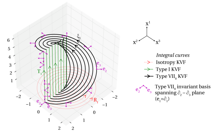
Figure 1: The Killing fields of Type VII₀ compared to those of Type I; some integral curves of both are shown (as thick and thin solid lines respectively). All the Type-I Killing fields ${\bm{\xi}}^{I}_{i}$ (along with ${\bm{\xi}}^{\mathrm{VII}_{0}}_{2}$ and ${\bm{\xi}}^{\mathrm{VII}_{0}}_{3}$) induce translations along the coordinate axes, whereas ${\bm{\xi}}^{\mathrm{VII}_{0}}_{1}$ (as a linear combination of $\partial_{1}$ and $R_{1}$) induces a more complex spiralling motion. The vectors of the invariant triad $\bi{e}_{2}^{\mathrm{VII}_{0}}$, $\bi{e}_{3}^{\mathrm{VII}_{0}}$ are also plotted. These spiral in response to the motion of the Killing fields; see equation (11).

The six Killing vector fields of flat space described by Cartesian coordinates $\{x^{i}\}$ are most simply expressed as the translations $\bi{T}_{i}=\partial_{i}$ and the rotations $\bi{R}_{i}=\epsilon_{ijk}x^{j}\partial_{k}$, with commutation relations

$$\left[\bi{T}_{i},\bi{T}_{j}\right]=0$$

$$\left[\bi{R}_{i},\bi{R}_{j}\right]=-\epsilon_{ijk}\bi{R}_{k}$$

$$\left[\bi{R}_{i},\bi{T}_{j}\right]=-\epsilon_{ijk}\bi{T}_{k}\textrm{.}$$ (8)

Solution of the closure requirement (2) in terms of the $\rho_{i}^{j}$ (5) leaves substantial freedom, but up to reparametrizations the two possibilities obtained give the Type-I and VII₀ KVFs (${\bm{\xi}}^{I}_{i}$ and ${\bm{\xi}}^{\mathrm{VII_{0}}}_{i}$ respectively) in canonical form:

$${\bm{\xi}}^{I}_{i}=\bi{T}_{i}$$ (9)

and

$${\bm{\xi}}^{\mathrm{VII_{0}}}_{1}=\bi{T}_{1}+\bi{R}_{1}$$

$${\bm{\xi}}^{\mathrm{VII_{0}}}_{j}=\bi{T}_{j}\hskip 56.9055ptj\neq 1\textrm{.}$$ (10)

The $\bi{T}_{i}$ have constant norm, form a subalgebra which is also closed under rotations and have geodesic integral curves; as noted in Section 2, these conditions are all equivalent. The Type-VII₀ KVFs do not satisfy such conditions, because integral curves of the ${\bm{\xi}}_{1}$ fields describe a spiralling motion (see Figure 1).

Because the background is flat, parallel transport of homogeneous quantities between different points on the manifold is uniquely defined; it may be verified that in the Type-I (but not VII₀) case the Lie transport coincides with parallel transport.

In the Type-I case, $\bi{T}_{i}$ are Abelian and so form their own reciprocal group. For Type VII₀, the reciprocal group is given by solving $[\bi{e}_{i},{\bm{\xi}}_{j}]=0$ subject to the constraint $\bi{e}_{i}|_{x=0}=\bi{{\bm{\xi}}}_{i}|_{x=0}$:

$$\left(\begin{array}[]{c}\bi{e}^{\mathrm{VII_{0}}}_{1}\\ \bi{e}^{\mathrm{VII_{0}}}_{2}\\ \bi{e}^{\mathrm{VII_{0}}}_{3}\end{array}\right)={\left(\begin{array}[]{ccc}\!1&0&0\\ 0&\cos x^{1}&\sin x^{1}\\ 0&-\sin x^{1}&\cos x^{1}\!\end{array}\right)}\left(\begin{array}[]{c}\partial_{1}\\ \partial_{2}\\ \partial_{3}\end{array}\right)\textrm{.}$$ (11)

These solutions are illustrated by plotting the vectors $\bi{e}^{\mathrm{VII_{0}}}_{2}$ and $\bi{e}^{\mathrm{VII_{0}}}_{3}$ at various points in Figure 1. Recalling that anisotropic quantities in the Type-VII₀ case will have constant components relative to the $\bi{e}^{\mathrm{VII_{0}}}_{i}$ basis, the origin of spiralling patterns in such universes becomes clear from inspecting this diagram.

3.2 Open space: Bianchi Types V and VII_h

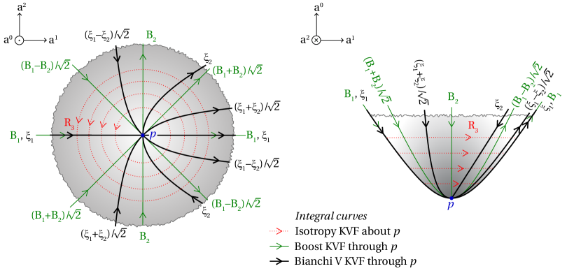
Figure 2: The open space as a hyperboloid embedded in Minkowski space; here a cut is taken along $a^{3}=0$, and a portion of the resulting geometry illustrated in two projections. In particular we plot integral curves of KVFs, decomposed about the point $p$ (where $a^{0}=1$) as described in the text. The rotational motion is shown as a dotted line, while boosts are shown as thin solid lines. However, the boosts do not form a closed group and thus do not qualify as generators of homogeneity according to the criteria in Section 2. Thus the Bianchi models take a linear combination of the boosts and rotations to form the basis set of Bianchi KVFs at $p$ (see equation 16). Here we have plotted integral curves of the Bianchi Type-V motions (heavy solid lines) which agree with the boosts in the tangent space of $p$, but deviate on scales of order the curvature radius. The rotational asymmetry of these integral curves, which is unavoidable in open models, ultimately leads to the non-trivial appearance of the Bianchi CMB.

To obtain coordinate expressions for the Killing and basis vectors, we consider the well-known embedding of an open manifold in Minkowski space. The ambient metric is

$$\mathrm{d}s^{2}=-\mathrm{d}(a^{0})^{2}+\mathrm{d}(a^{1})^{2}+\mathrm{d}(a^{2})^{2}+\mathrm{d}(a^{3})^{2}\textrm{.}$$ (12)

The hypersurface representing the open space, with curvature set to $1$ without loss of generality, is defined by

$$1=(a^{0})^{2}-\left[(a^{1})^{2}+(a^{2})^{2}+(a^{3})^{2}\right]\textrm{.}$$ (13)

The group of continuous global linear transformations which preserve (12, 13) is the restricted Lorentz group SO${}^{+}(3,1)$. There are six Killing vector fields which can be decomposed about a point $p$ into three rotations ($\bi{R}_{i}$) and three boosts ($\bi{B}_{i}$):

$$\bi{R}_{i}=\epsilon_{ijk}a^{j}\partial_{k}$$

$$\bi{B}_{i}=a^{i}\partial_{0}+a^{0}\partial_{i}\textrm{,}$$ (14)

where the special point is taken without loss of generality to be $a^{0}=1$, $a^{i}=0$ ($i>0$). These Killing fields have well-known commutators:

$$\left[\bi{R}_{i},\bi{R}_{j}\right] = -\epsilon_{ijk}\bi{R}_{k}$$

$$\left[\bi{B}_{i},\bi{B}_{j}\right] = \epsilon_{ijk}\bi{R}_{k}$$

$$\left[\bi{R}_{i},\bi{B}_{j}\right] = -\epsilon_{ijk}\bi{B}_{k}\textrm{.}$$ (15)

The commutation relations (15) show that the boosts $\bi{B}_{i}$ are not suitable generators for homogeneity because they do not form a closed group. One must therefore consider linear combinations of the form (5). It may be verified that the only closed possibilities (unique up to transformations under the isotropy subgroup $\{\bi{R}_{i}\}$) give either a realisation of the canonical Type-V or VII_h KVFs. In the former case we have

$$\bi{{\bm{\xi}}}^{\mathrm{V}}_{1}=\bi{B}_{1},\qquad\bi{{\bm{\xi}}}^{\mathrm{V}}_{2}=\bi{B}_{2}-\bi{R}_{3},\qquad\bi{{\bm{\xi}}}^{\mathrm{V}}_{3}=\bi{B}_{3}+\bi{R}_{2}\textrm{.}$$ (16)

The effect of this choice is shown in Figure 2 by displaying the hyperboloid described in the space spanned by the $a^{i}$ coordinates (taking $a^{3}=0$). In particular, we have illustrated integral curves through $p$ of both the $\bi{B}_{1}$, $\bi{B}_{2}$ subset (thin solid lines) and the ${\bm{\xi}}_{1}$, ${\bm{\xi}}_{2}$ subset (heavy solid lines). Both of these sets span the $a^{1},a^{2}$ tangent space at $p$ which allows for a direct comparison. While the $\bi{B}_{i}$ subset is closed under rotations, this is not the case for the ${\bm{\xi}}_{i}$ subset; for instance, it is clear from the figure that ${\bm{\xi}}_{2}$ is not obtained from any rotation about $p$ of ${\bm{\xi}}_{1}$. We emphasize again that, despite their attractive qualities, the $\bi{B}_{i}$ are not suitable for transporting anisotropic quantities since they do not form a closed subalgebra (Section 2).

For Type VII_h one has

$$\bi{{\bm{\xi}}}^{\mathrm{VII}_{h}}_{1}=\sqrt{h}\,\bi{{\bm{\xi}}}_{1}^{\mathrm{V}}+\bi{R}_{1}$$

$$\bi{{\bm{\xi}}}^{\mathrm{VII}_{h}}_{j}=\sqrt{h}\,\bi{{\bm{\xi}}}^{\mathrm{V}}_{j}\hskip 85.35826pt(j\neq 1)\textrm{.}$$ (17)

Note the similarity of the relation (3.1) between Type-I and VII₀ Killing fields with the relation (17) between Type V and VII_h. Both introduce a ‘spiralling’ motion into one of the Killing fields. In the flat case, this is fixed (in the canonical decomposition) to have a unit comoving scale length which is later adjusted in physical scale by the choice of spatial scale-factor at redshift zero. In the open case, there is an additional freedom in the relative scale of the isotropic curvature and spiral motion; this is fixed by adjusting the value of the structure constant $\sqrt{h}$.

We can find invariant vectors by solving $[\bi{{\bm{\xi}}}_{i},\bi{e}_{j}]=0$ subject to the constraint $\bi{e}_{i}={\bm{\xi}}_{i}$ at $a^{0}=1$. For Type V, we find

$$\bi{e}^{\mathrm{V}}_{1} = \left(e^{x}-a^{0}\right)\partial_{0}+\left(e^{x}-a^{1}\right)\partial_{1}-a^{2}\partial_{2}-a^{3}\partial_{3}$$

$$\bi{e}^{\mathrm{V}}_{2} = e^{x}{\bm{\xi}}^{\mathrm{V}}_{2}$$

$$\bi{e}^{\mathrm{V}}_{3} = e^{x}{\bm{\xi}}^{\mathrm{V}}_{3},$$ (18)

where $x=-\ln(a^{0}-a^{1})$. (For a geometrical interpretation of $x$, see A.1.) For VII_h, a suitable invariant basis is

$$\left(\begin{array}[]{c}\bi{e}^{\mathrm{VII}_{h}}_{1}\\ \bi{e}^{\mathrm{VII}_{h}}_{2}\\ \bi{e}^{\mathrm{VII}_{h}}_{3}\end{array}\right)=\sqrt{h}{\left(\begin{array}[]{ccc}\!1&0&0\\ 0&\cos(x/\sqrt{h})&\sin(x/\sqrt{h})\\ 0&-\sin(x/\sqrt{h})&\cos(x/\sqrt{h})\!\end{array}\right)}\left(\begin{array}[]{c}\bi{e}^{\mathrm{V}}_{1}\\ \bi{e}^{\mathrm{V}}_{2}\\ \bi{e}^{\mathrm{V}}_{3}\end{array}\right).$$ (19)

This simple formulation arises because the ${\bm{\xi}}_{i}$ are closed under the action of $\bi{R}_{1}$, so the Jacobi identities applied to $0=[\bi{R}_{1},[{\bm{\xi}}_{j},\bi{e}_{k}]]$ may be used to show that the $\{\bi{e}^{V}_{i}\}$ are closed under the action of $\bi{R}_{1}$. The corresponding commutation coefficients are fixed by the behaviour of $\bi{R}_{i}$ on the tangent space at the identity, i.e. $[\bi{R}_{1},\bi{e}_{1}^{\mathrm{V}}]=0$, $[\bi{R}_{1},\bi{e}_{2}^{\mathrm{V}}]=-\bi{e}^{\mathrm{V}}_{3}$, $[\bi{R}_{1},\bi{e}_{3}^{\mathrm{V}}]=\bi{e}^{\mathrm{V}}_{2}$. (These may be verified directly from equation 18.) The construction is therefore completely analogous to that of the VII₀ invariant fields.

3.3 Closed space: Bianchi type IX

The closed case has been discussed extensively in Ref. [19]. A suitable embedding may be considered with the ambient metric and surface function

$$\mathrm{d}s^{2}=(\mathrm{d}a^{0})^{2}+(\mathrm{d}a^{1})^{2}+(\mathrm{d}a^{2})^{2}+(\mathrm{d}a^{3})^{2}$$

$$1=(a^{0})^{2}+(a^{1})^{2}+(a^{2})^{2}+(a^{3})^{2}\textrm{,}$$ (20)

with KVFs

$$\bi{R}_{i}=\epsilon_{ijk}a^{j}\partial_{k}$$

$$\bi{T}_{i}=a^{i}\partial_{0}-a^{0}\partial_{i}\textrm{.}$$ (21)

The commutation relations are

$$\left[\bi{R}_{i},\bi{R}_{j}\right]=-\epsilon_{ijk}\bi{R}_{k}$$

$$\left[\bi{T}_{i},\bi{T}_{j}\right]=-\epsilon_{ijk}\bi{R}_{k}$$

$$\left[\bi{R}_{i},\bi{T}_{j}\right]=-\epsilon_{ijk}\bi{T}_{k}\textrm{.}$$ (22)

In the vicinity of $a^{0}=1$, $a^{i}=0$, the $\bi{T}_{i}$ correspond to Euclidean translations along the $i$th coordinate direction and the $\bi{R}_{i}$ correspond to rotations about $a^{0}=1$, $a^{i}=0$.

There are two simply-transitive subgroups

$${\bm{\xi}}^{\pm}_{i}=\frac{1}{2}\left(\bi{T}_{i}\pm\bi{R}_{i}\right),$$ (23)

and both yield Type-IX structure constants:

$$\left[{\bm{\xi}}^{\pm}_{i},{\bm{\xi}}^{\pm}_{j}\right]=\mp\epsilon_{ijk}{\bm{\xi}}^{\pm}_{k}.$$ (24)

With the factor $1/2$ in (23), the ${\bm{\xi}}^{+}_{i}$ have canonical commutation relations, while reversing the sign of the ${\bm{\xi}}^{-}_{i}$ makes this set canonical too. One may verify that both sets of Killing vector fields have constant norm on the surface, so are tangent to congruences of geodesics as described for the flat case above. From this it follows that parallel transport and Lie transport along a Killing field can differ only by a rotation in the plane perpendicular to the transport direction. This behaviour can succinctly account for the appearance of the CMB in Type-IX models: the temperature pattern is a pure quadrupole but a screen-projected polarization vector spirals at a constant rate in conformal time [12]. (However, for an exception to this behaviour see the near-VII₀ models in Section 6.)

Since $[{\bm{\xi}}^{+}_{i},{\bm{\xi}}^{-}_{j}]=0$, the invariant fields are also Killing (the metric is bi-invariant; it is, actually, the Killing metric for this space). For consistency we should adopt ${\bm{\xi}}^{\mathrm{IX}}_{i}={\bm{\xi}}^{+}_{i}$, $\bi{e}^{\mathrm{IX}}_{i}={\bm{\xi}}^{-}_{i}$, although these roles are reversed under parity.

4 Enumerating the linearised Bianchi modes

In this section, we present a derivation of the independent modes which could arise in an almost-isotropic Universe consistent with Bianchi-type symmetries.

Our starting point is the metric in equation (7). We can break isotropy while preserving homogeneity by adding a spatial metric perturbation of the form

$$\delta g=\delta{g}_{ab}(t)\bi{e}^{a}\otimes\bi{e}^{b}\,.$$ (25)

As described in Section 2, the perturbed metric is invariant under the action of the homogeneity group, which is a subgroup of the original isometries for the unperturbed FRW spacetime. The full, perturbed metric can be written in the form [22, 25]

$$g=-\tilde{\bi{n}}\otimes\tilde{\bi{n}}+e^{2\alpha(t)}(e^{2\beta(t)})_{ab}\bi{e}^{a}\otimes\bi{e}^{b}\,,$$ (26)

where the symmetric, trace-free (STF) $\beta_{ab}(t)$ and, generally, $\alpha(t)$ are perturbed from their FRW values. By construction, the isotropic limit corresponds to $\beta_{ab}=\dot{\beta}_{ab}=0$, where an overdot denotes the derivative with respect to $t$. The evolution of $\beta$ contains all information about the anisotropic perturbation (at any order).

The evolution (Einstein) equations are most simply expressed relative to an orthonormal frame, denoted $\hat{\bi{e}}_{\hat{a}}$. One may construct such a frame explicitly [22] via the transformation

$$\hat{\bi{e}}_{\hat{a}}=e^{-\alpha}\left(e^{-\beta}\right)_{\hat{a}a}\bi{e}_{a}\textrm{.}$$ (27)

The expansion $H$, shear $\sigma_{\hat{a}\hat{b}}$ and Fermi-relative rotation $\Omega_{\hat{a}}$ of the orthonormal frame are defined by

$$\bi{e}_{\hat{a}}\cdot[\bi{n},\bi{e}_{\hat{b}}]=-H\delta_{\hat{a}\hat{b}}-\sigma_{\hat{a}\hat{b}}-\epsilon_{\hat{a}\hat{b}\hat{c}}\Omega^{\hat{c}}\textrm{,}$$ (28)

where $\sigma_{\hat{a}\hat{b}}$ is symmetric and trace-free. We shall now linearise about the background FRW solution by requiring

$$\left|\beta_{ab}\right| =\mathcal{O}(\epsilon)$$

$$\left|\dot{\beta}_{ab}/H\right| =\mathcal{O}(\epsilon)$$

$$e^{-2\alpha}\left|\beta_{ab}C^{2}/H^{2}\right| =\mathcal{O}(\epsilon)\,,$$ (29)

where $\epsilon\ll 1$. The final condition can be interpreted as putting a lower bound on the wavelength of the perturbations as a fraction of the horizon size, which is necessary for spatial derivatives of perturbed quantities to remain small. We perform a fiducial fluid decomposition of the stress tensor as

$$T_{\mu\nu}=\rho n_{\mu}n_{\nu}+p(g_{\mu\nu}+n_{\mu}n_{\nu})+2n_{(\mu}P_{\nu)}+\pi_{\mu\nu},$$ (30)

where $\rho$ is the fluid energy density measured by observers comoving with the $\bi{n}$ congruence, $p$ the isotropic pressure, $P_{\mu}$ the momentum density and $\pi_{\mu\nu}$ the anisotropic stress. Here $P_{\mu}$ and $\pi_{\mu\nu}$ are orthogonal to $\bi{n}$ ($P_{\mu}n^{\mu}=\pi_{\mu\nu}n^{\nu}=0$) and $\pi_{\mu\nu}$ is symmetric and trace-free. We further assume

$$\left|\pi_{\mu\nu}/H^{2}\right|=\mathcal{O}(\epsilon),\qquad\left|P_{\mu}/H^{2}\right|=\mathcal{O}(\epsilon)\,,$$ (31)

and will in practice shortly restrict $\pi_{\mu\nu}=0$, i.e. a perfect fluid, although unlike many Bianchi model analyses we will allow for small non-zero momentum density $P_{\mu}$ (corresponding to tilt of the fluid source).

The first-order kinematic and dynamical quantities in the orthonormal frame are

$$e^{\alpha}\hat{a}_{\hat{a}} =a_{\hat{a}}-\beta_{\hat{a}a}a_{a}+\mathcal{O}(\epsilon^{2})$$ (32)

$$e^{\alpha}\hat{n}^{\hat{a}\hat{b}} =n^{\hat{a}\hat{b}}+\beta_{\hat{a}a}n^{a\hat{b}}+\beta_{\hat{b}b}n^{\hat{a}b}+\mathcal{O}(\epsilon^{2})$$ (33)

$$\sigma_{\hat{a}\hat{b}}/H =\dot{\beta}_{\hat{a}\hat{b}}/H+\mathcal{O}(\epsilon^{2})$$ (34)

$$H =\dot{\alpha}$$ (35)

$$\Omega_{\hat{c}}/H =\mathcal{O}(\epsilon^{2})\textrm{.}$$ (36)

These equations are non-tensorial (valid only in the orthonormal frame); the components of $a$ and $n$ on the right-hand sides are the canonical, time-invariant structure constants and the components of $\beta_{ab}$ are as defined in the time-invariant frame.

The expansions above may be inserted directly into the orthonormal-frame Einstein equations (see, e.g., Ref. [2]; or for a somewhat different form, Ref. [26]), giving

$$\rho =3H^{2}+\mathchoice{\hphantom{{}^{\leavevmode{3}}_{\mathchoice{\makebox[3.5pt][c]{$\displaystyle$}}{\makebox[3.5pt][c]{$\textstyle$}}{\makebox[2.45pt][c]{$\scriptstyle$}}{\makebox[1.75pt][c]{$\scriptscriptstyle$}}}}R^{\kern-6.9402pt\leavevmode{3}\kern 5.3691pt}_{\kern-11.2522pt\mathchoice{\makebox[3.5pt][c]{$\displaystyle$}}{\makebox[3.5pt][c]{$\textstyle$}}{\makebox[2.45pt][c]{$\scriptstyle$}}{\makebox[1.75pt][c]{$\scriptscriptstyle$}}\kern 5.3691pt}}{\hphantom{{}^{\leavevmode{3}}_{\mathchoice{\makebox[3.5pt][c]{$\displaystyle$}}{\makebox[3.5pt][c]{$\textstyle$}}{\makebox[2.45pt][c]{$\scriptstyle$}}{\makebox[1.75pt][c]{$\scriptscriptstyle$}}}}R^{\kern-6.9402pt\leavevmode{3}\kern 5.3691pt}_{\kern-11.2522pt\mathchoice{\makebox[3.5pt][c]{$\displaystyle$}}{\makebox[3.5pt][c]{$\textstyle$}}{\makebox[2.45pt][c]{$\scriptstyle$}}{\makebox[1.75pt][c]{$\scriptscriptstyle$}}\kern 5.3691pt}}{\hphantom{{}^{\leavevmode{3}}_{\mathchoice{\makebox[3.5pt][c]{$\displaystyle$}}{\makebox[3.5pt][c]{$\textstyle$}}{\makebox[2.45pt][c]{$\scriptstyle$}}{\makebox[1.75pt][c]{$\scriptscriptstyle$}}}}R^{\kern-4.76945pt\leavevmode{3}\kern 3.75835pt}_{\kern-7.84946pt\mathchoice{\makebox[3.5pt][c]{$\displaystyle$}}{\makebox[3.5pt][c]{$\textstyle$}}{\makebox[2.45pt][c]{$\scriptstyle$}}{\makebox[1.75pt][c]{$\scriptscriptstyle$}}\kern 3.75835pt}}{\hphantom{{}^{\leavevmode{3}}_{\mathchoice{\makebox[3.5pt][c]{$\displaystyle$}}{\makebox[3.5pt][c]{$\textstyle$}}{\makebox[2.45pt][c]{$\scriptstyle$}}{\makebox[1.75pt][c]{$\scriptscriptstyle$}}}}R^{\kern-3.69565pt\leavevmode{3}\kern 2.68454pt}_{\kern-6.77565pt\mathchoice{\makebox[3.5pt][c]{$\displaystyle$}}{\makebox[3.5pt][c]{$\textstyle$}}{\makebox[2.45pt][c]{$\scriptstyle$}}{\makebox[1.75pt][c]{$\scriptscriptstyle$}}\kern 2.68454pt}}/2-\Lambda+\mathcal{O}(H^{2}\epsilon^{2})$$ (37)

$$\dot{H} =-H^{2}-(\rho+3p)/6+\Lambda/3+\mathcal{O}(H^{2}\epsilon^{2})$$ (38)

$$\ddot{\beta}_{\hat{a}\hat{b}} =-3H\dot{\beta}_{\hat{a}\hat{b}}-\mathchoice{\hphantom{{}^{\leavevmode{3}}_{\mathchoice{\makebox[3.5pt][c]{$\displaystyle$}}{\makebox[3.5pt][c]{$\textstyle$}}{\makebox[2.45pt][c]{$\scriptstyle$}}{\makebox[1.75pt][c]{$\scriptscriptstyle$}}}}S^{\kern-6.26692pt\leavevmode{3}\kern 4.69582pt\mathchoice{\makebox[11.11115pt][c]{$\displaystyle$}}{\makebox[11.11115pt][c]{$\textstyle$}}{\makebox[11.11115pt][c]{$\scriptstyle$}}{\makebox[11.11115pt][c]{$\scriptscriptstyle$}}}_{\kern-10.57892pt\mathchoice{\makebox[3.5pt][c]{$\displaystyle$}}{\makebox[3.5pt][c]{$\textstyle$}}{\makebox[2.45pt][c]{$\scriptstyle$}}{\makebox[1.75pt][c]{$\scriptscriptstyle$}}\kern 4.69582pt\leavevmode{\hat{a}\hat{b}}}}{\hphantom{{}^{\leavevmode{3}}_{\mathchoice{\makebox[3.5pt][c]{$\displaystyle$}}{\makebox[3.5pt][c]{$\textstyle$}}{\makebox[2.45pt][c]{$\scriptstyle$}}{\makebox[1.75pt][c]{$\scriptscriptstyle$}}}}S^{\kern-6.26692pt\leavevmode{3}\kern 4.69582pt\mathchoice{\makebox[11.11115pt][c]{$\displaystyle$}}{\makebox[11.11115pt][c]{$\textstyle$}}{\makebox[11.11115pt][c]{$\scriptstyle$}}{\makebox[11.11115pt][c]{$\scriptscriptstyle$}}}_{\kern-10.57892pt\mathchoice{\makebox[3.5pt][c]{$\displaystyle$}}{\makebox[3.5pt][c]{$\textstyle$}}{\makebox[2.45pt][c]{$\scriptstyle$}}{\makebox[1.75pt][c]{$\scriptscriptstyle$}}\kern 4.69582pt\leavevmode{\hat{a}\hat{b}}}}{\hphantom{{}^{\leavevmode{3}}_{\mathchoice{\makebox[3.5pt][c]{$\displaystyle$}}{\makebox[3.5pt][c]{$\textstyle$}}{\makebox[2.45pt][c]{$\scriptstyle$}}{\makebox[1.75pt][c]{$\scriptscriptstyle$}}}}S^{\kern-4.29819pt\leavevmode{3}\kern 3.28708pt\mathchoice{\makebox[11.11115pt][c]{$\displaystyle$}}{\makebox[11.11115pt][c]{$\textstyle$}}{\makebox[11.11115pt][c]{$\scriptstyle$}}{\makebox[11.11115pt][c]{$\scriptscriptstyle$}}}_{\kern-7.37819pt\mathchoice{\makebox[3.5pt][c]{$\displaystyle$}}{\makebox[3.5pt][c]{$\textstyle$}}{\makebox[2.45pt][c]{$\scriptstyle$}}{\makebox[1.75pt][c]{$\scriptscriptstyle$}}\kern 3.28708pt\leavevmode{\hat{a}\hat{b}}}}{\hphantom{{}^{\leavevmode{3}}_{\mathchoice{\makebox[3.5pt][c]{$\displaystyle$}}{\makebox[3.5pt][c]{$\textstyle$}}{\makebox[2.45pt][c]{$\scriptstyle$}}{\makebox[1.75pt][c]{$\scriptscriptstyle$}}}}S^{\kern-3.35901pt\leavevmode{3}\kern 2.3479pt\mathchoice{\makebox[11.11115pt][c]{$\displaystyle$}}{\makebox[11.11115pt][c]{$\textstyle$}}{\makebox[11.11115pt][c]{$\scriptstyle$}}{\makebox[11.11115pt][c]{$\scriptscriptstyle$}}}_{\kern-6.43901pt\mathchoice{\makebox[3.5pt][c]{$\displaystyle$}}{\makebox[3.5pt][c]{$\textstyle$}}{\makebox[2.45pt][c]{$\scriptstyle$}}{\makebox[1.75pt][c]{$\scriptscriptstyle$}}\kern 2.3479pt\leavevmode{\hat{a}\hat{b}}}}+\pi_{\hat{a}\hat{b}}+\mathcal{O}(H^{2}\epsilon^{2})$$ (39)

$$P_{\hat{a}} =e^{-\alpha}\left(3\dot{\beta}_{\hat{a}b}a_{b}-\epsilon_{\hat{a}bc}\dot{\beta}_{bd}n_{dc}\right)+\mathcal{O}(e^{-\alpha}HC\epsilon^{2})\textrm{,}$$ (40)

with the fluid conservation equation

$$\dot{\rho}=-3H(\rho+p)+2e^{-\alpha}a_{\hat{a}}P^{\hat{a}}+\mathcal{O}(e^{-2\alpha}HC^{2}\epsilon^{2},H^{3}\epsilon^{2})\textrm{,}$$ (41)

where the structure constants $a$ and $n$ again take their canonical numerical values. In equations (37) and (38), $\mathchoice{\hphantom{{}^{\leavevmode{3}}_{\mathchoice{\makebox[3.5pt][c]{$\displaystyle$}}{\makebox[3.5pt][c]{$\textstyle$}}{\makebox[2.45pt][c]{$\scriptstyle$}}{\makebox[1.75pt][c]{$\scriptscriptstyle$}}}}R^{\kern-6.9402pt\leavevmode{3}\kern 5.3691pt}_{\kern-11.2522pt\mathchoice{\makebox[3.5pt][c]{$\displaystyle$}}{\makebox[3.5pt][c]{$\textstyle$}}{\makebox[2.45pt][c]{$\scriptstyle$}}{\makebox[1.75pt][c]{$\scriptscriptstyle$}}\kern 5.3691pt}}{\hphantom{{}^{\leavevmode{3}}_{\mathchoice{\makebox[3.5pt][c]{$\displaystyle$}}{\makebox[3.5pt][c]{$\textstyle$}}{\makebox[2.45pt][c]{$\scriptstyle$}}{\makebox[1.75pt][c]{$\scriptscriptstyle$}}}}R^{\kern-6.9402pt\leavevmode{3}\kern 5.3691pt}_{\kern-11.2522pt\mathchoice{\makebox[3.5pt][c]{$\displaystyle$}}{\makebox[3.5pt][c]{$\textstyle$}}{\makebox[2.45pt][c]{$\scriptstyle$}}{\makebox[1.75pt][c]{$\scriptscriptstyle$}}\kern 5.3691pt}}{\hphantom{{}^{\leavevmode{3}}_{\mathchoice{\makebox[3.5pt][c]{$\displaystyle$}}{\makebox[3.5pt][c]{$\textstyle$}}{\makebox[2.45pt][c]{$\scriptstyle$}}{\makebox[1.75pt][c]{$\scriptscriptstyle$}}}}R^{\kern-4.76945pt\leavevmode{3}\kern 3.75835pt}_{\kern-7.84946pt\mathchoice{\makebox[3.5pt][c]{$\displaystyle$}}{\makebox[3.5pt][c]{$\textstyle$}}{\makebox[2.45pt][c]{$\scriptstyle$}}{\makebox[1.75pt][c]{$\scriptscriptstyle$}}\kern 3.75835pt}}{\hphantom{{}^{\leavevmode{3}}_{\mathchoice{\makebox[3.5pt][c]{$\displaystyle$}}{\makebox[3.5pt][c]{$\textstyle$}}{\makebox[2.45pt][c]{$\scriptstyle$}}{\makebox[1.75pt][c]{$\scriptscriptstyle$}}}}R^{\kern-3.69565pt\leavevmode{3}\kern 2.68454pt}_{\kern-6.77565pt\mathchoice{\makebox[3.5pt][c]{$\displaystyle$}}{\makebox[3.5pt][c]{$\textstyle$}}{\makebox[2.45pt][c]{$\scriptstyle$}}{\makebox[1.75pt][c]{$\scriptscriptstyle$}}\kern 2.68454pt}}$ and ${}^{3}S_{\hat{a}\hat{b}}=\mathchoice{\hphantom{{}^{\leavevmode{3}}_{\mathchoice{\makebox[3.5pt][c]{$\displaystyle$}}{\makebox[3.5pt][c]{$\textstyle$}}{\makebox[2.45pt][c]{$\scriptstyle$}}{\makebox[1.75pt][c]{$\scriptscriptstyle$}}}}R^{\kern-6.9402pt\leavevmode{3}\kern 5.3691pt\mathchoice{\makebox[11.11115pt][c]{$\displaystyle$}}{\makebox[11.11115pt][c]{$\textstyle$}}{\makebox[11.11115pt][c]{$\scriptstyle$}}{\makebox[11.11115pt][c]{$\scriptscriptstyle$}}}_{\kern-11.2522pt\mathchoice{\makebox[3.5pt][c]{$\displaystyle$}}{\makebox[3.5pt][c]{$\textstyle$}}{\makebox[2.45pt][c]{$\scriptstyle$}}{\makebox[1.75pt][c]{$\scriptscriptstyle$}}\kern 5.3691pt\leavevmode{\hat{a}\hat{b}}}}{\hphantom{{}^{\leavevmode{3}}_{\mathchoice{\makebox[3.5pt][c]{$\displaystyle$}}{\makebox[3.5pt][c]{$\textstyle$}}{\makebox[2.45pt][c]{$\scriptstyle$}}{\makebox[1.75pt][c]{$\scriptscriptstyle$}}}}R^{\kern-6.9402pt\leavevmode{3}\kern 5.3691pt\mathchoice{\makebox[11.11115pt][c]{$\displaystyle$}}{\makebox[11.11115pt][c]{$\textstyle$}}{\makebox[11.11115pt][c]{$\scriptstyle$}}{\makebox[11.11115pt][c]{$\scriptscriptstyle$}}}_{\kern-11.2522pt\mathchoice{\makebox[3.5pt][c]{$\displaystyle$}}{\makebox[3.5pt][c]{$\textstyle$}}{\makebox[2.45pt][c]{$\scriptstyle$}}{\makebox[1.75pt][c]{$\scriptscriptstyle$}}\kern 5.3691pt\leavevmode{\hat{a}\hat{b}}}}{\hphantom{{}^{\leavevmode{3}}_{\mathchoice{\makebox[3.5pt][c]{$\displaystyle$}}{\makebox[3.5pt][c]{$\textstyle$}}{\makebox[2.45pt][c]{$\scriptstyle$}}{\makebox[1.75pt][c]{$\scriptscriptstyle$}}}}R^{\kern-4.76945pt\leavevmode{3}\kern 3.75835pt\mathchoice{\makebox[11.11115pt][c]{$\displaystyle$}}{\makebox[11.11115pt][c]{$\textstyle$}}{\makebox[11.11115pt][c]{$\scriptstyle$}}{\makebox[11.11115pt][c]{$\scriptscriptstyle$}}}_{\kern-7.84946pt\mathchoice{\makebox[3.5pt][c]{$\displaystyle$}}{\makebox[3.5pt][c]{$\textstyle$}}{\makebox[2.45pt][c]{$\scriptstyle$}}{\makebox[1.75pt][c]{$\scriptscriptstyle$}}\kern 3.75835pt\leavevmode{\hat{a}\hat{b}}}}{\hphantom{{}^{\leavevmode{3}}_{\mathchoice{\makebox[3.5pt][c]{$\displaystyle$}}{\makebox[3.5pt][c]{$\textstyle$}}{\makebox[2.45pt][c]{$\scriptstyle$}}{\makebox[1.75pt][c]{$\scriptscriptstyle$}}}}R^{\kern-3.69565pt\leavevmode{3}\kern 2.68454pt\mathchoice{\makebox[11.11115pt][c]{$\displaystyle$}}{\makebox[11.11115pt][c]{$\textstyle$}}{\makebox[11.11115pt][c]{$\scriptstyle$}}{\makebox[11.11115pt][c]{$\scriptscriptstyle$}}}_{\kern-6.77565pt\mathchoice{\makebox[3.5pt][c]{$\displaystyle$}}{\makebox[3.5pt][c]{$\textstyle$}}{\makebox[2.45pt][c]{$\scriptstyle$}}{\makebox[1.75pt][c]{$\scriptscriptstyle$}}\kern 2.68454pt\leavevmode{\hat{a}\hat{b}}}}-\mathchoice{\hphantom{{}^{\leavevmode{3}}_{\mathchoice{\makebox[3.5pt][c]{$\displaystyle$}}{\makebox[3.5pt][c]{$\textstyle$}}{\makebox[2.45pt][c]{$\scriptstyle$}}{\makebox[1.75pt][c]{$\scriptscriptstyle$}}}}R^{\kern-6.9402pt\leavevmode{3}\kern 5.3691pt}_{\kern-11.2522pt\mathchoice{\makebox[3.5pt][c]{$\displaystyle$}}{\makebox[3.5pt][c]{$\textstyle$}}{\makebox[2.45pt][c]{$\scriptstyle$}}{\makebox[1.75pt][c]{$\scriptscriptstyle$}}\kern 5.3691pt}}{\hphantom{{}^{\leavevmode{3}}_{\mathchoice{\makebox[3.5pt][c]{$\displaystyle$}}{\makebox[3.5pt][c]{$\textstyle$}}{\makebox[2.45pt][c]{$\scriptstyle$}}{\makebox[1.75pt][c]{$\scriptscriptstyle$}}}}R^{\kern-6.9402pt\leavevmode{3}\kern 5.3691pt}_{\kern-11.2522pt\mathchoice{\makebox[3.5pt][c]{$\displaystyle$}}{\makebox[3.5pt][c]{$\textstyle$}}{\makebox[2.45pt][c]{$\scriptstyle$}}{\makebox[1.75pt][c]{$\scriptscriptstyle$}}\kern 5.3691pt}}{\hphantom{{}^{\leavevmode{3}}_{\mathchoice{\makebox[3.5pt][c]{$\displaystyle$}}{\makebox[3.5pt][c]{$\textstyle$}}{\makebox[2.45pt][c]{$\scriptstyle$}}{\makebox[1.75pt][c]{$\scriptscriptstyle$}}}}R^{\kern-4.76945pt\leavevmode{3}\kern 3.75835pt}_{\kern-7.84946pt\mathchoice{\makebox[3.5pt][c]{$\displaystyle$}}{\makebox[3.5pt][c]{$\textstyle$}}{\makebox[2.45pt][c]{$\scriptstyle$}}{\makebox[1.75pt][c]{$\scriptscriptstyle$}}\kern 3.75835pt}}{\hphantom{{}^{\leavevmode{3}}_{\mathchoice{\makebox[3.5pt][c]{$\displaystyle$}}{\makebox[3.5pt][c]{$\textstyle$}}{\makebox[2.45pt][c]{$\scriptstyle$}}{\makebox[1.75pt][c]{$\scriptscriptstyle$}}}}R^{\kern-3.69565pt\leavevmode{3}\kern 2.68454pt}_{\kern-6.77565pt\mathchoice{\makebox[3.5pt][c]{$\displaystyle$}}{\makebox[3.5pt][c]{$\textstyle$}}{\makebox[2.45pt][c]{$\scriptstyle$}}{\makebox[1.75pt][c]{$\scriptscriptstyle$}}\kern 2.68454pt}}\delta_{\hat{a}\hat{b}}/3$ are the isotropic and anisotropic parts of the spatial 3-curvature respectively:

$${}^{3}Re^{2\alpha} = \mathchoice{\hphantom{{}^{\leavevmode{3}}_{\mathchoice{\makebox[3.5pt][c]{$\displaystyle$}}{\makebox[3.5pt][c]{$\textstyle$}}{\makebox[2.45pt][c]{$\scriptstyle$}}{\makebox[1.75pt][c]{$\scriptscriptstyle$}}}}R^{\kern-6.9402pt\leavevmode{3}\kern 5.3691pt\leavevmode{\hat{a}}\mathchoice{\makebox[5.55557pt][c]{$\displaystyle$}}{\makebox[5.55557pt][c]{$\textstyle$}}{\makebox[5.55557pt][c]{$\scriptstyle$}}{\makebox[5.55557pt][c]{$\scriptscriptstyle$}}}_{\kern-11.2522pt\mathchoice{\makebox[3.5pt][c]{$\displaystyle$}}{\makebox[3.5pt][c]{$\textstyle$}}{\makebox[2.45pt][c]{$\scriptstyle$}}{\makebox[1.75pt][c]{$\scriptscriptstyle$}}\kern 5.3691pt\mathchoice{\makebox[5.55557pt][c]{$\displaystyle$}}{\makebox[5.55557pt][c]{$\textstyle$}}{\makebox[5.55557pt][c]{$\scriptstyle$}}{\makebox[5.55557pt][c]{$\scriptscriptstyle$}}\leavevmode{\hat{a}}}}{\hphantom{{}^{\leavevmode{3}}_{\mathchoice{\makebox[3.5pt][c]{$\displaystyle$}}{\makebox[3.5pt][c]{$\textstyle$}}{\makebox[2.45pt][c]{$\scriptstyle$}}{\makebox[1.75pt][c]{$\scriptscriptstyle$}}}}R^{\kern-6.9402pt\leavevmode{3}\kern 5.3691pt\leavevmode{\hat{a}}\mathchoice{\makebox[5.55557pt][c]{$\displaystyle$}}{\makebox[5.55557pt][c]{$\textstyle$}}{\makebox[5.55557pt][c]{$\scriptstyle$}}{\makebox[5.55557pt][c]{$\scriptscriptstyle$}}}_{\kern-11.2522pt\mathchoice{\makebox[3.5pt][c]{$\displaystyle$}}{\makebox[3.5pt][c]{$\textstyle$}}{\makebox[2.45pt][c]{$\scriptstyle$}}{\makebox[1.75pt][c]{$\scriptscriptstyle$}}\kern 5.3691pt\mathchoice{\makebox[5.55557pt][c]{$\displaystyle$}}{\makebox[5.55557pt][c]{$\textstyle$}}{\makebox[5.55557pt][c]{$\scriptstyle$}}{\makebox[5.55557pt][c]{$\scriptscriptstyle$}}\leavevmode{\hat{a}}}}{\hphantom{{}^{\leavevmode{3}}_{\mathchoice{\makebox[3.5pt][c]{$\displaystyle$}}{\makebox[3.5pt][c]{$\textstyle$}}{\makebox[2.45pt][c]{$\scriptstyle$}}{\makebox[1.75pt][c]{$\scriptscriptstyle$}}}}R^{\kern-4.76945pt\leavevmode{3}\kern 3.75835pt\leavevmode{\hat{a}}\mathchoice{\makebox[5.55557pt][c]{$\displaystyle$}}{\makebox[5.55557pt][c]{$\textstyle$}}{\makebox[5.55557pt][c]{$\scriptstyle$}}{\makebox[5.55557pt][c]{$\scriptscriptstyle$}}}_{\kern-7.84946pt\mathchoice{\makebox[3.5pt][c]{$\displaystyle$}}{\makebox[3.5pt][c]{$\textstyle$}}{\makebox[2.45pt][c]{$\scriptstyle$}}{\makebox[1.75pt][c]{$\scriptscriptstyle$}}\kern 3.75835pt\mathchoice{\makebox[5.55557pt][c]{$\displaystyle$}}{\makebox[5.55557pt][c]{$\textstyle$}}{\makebox[5.55557pt][c]{$\scriptstyle$}}{\makebox[5.55557pt][c]{$\scriptscriptstyle$}}\leavevmode{\hat{a}}}}{\hphantom{{}^{\leavevmode{3}}_{\mathchoice{\makebox[3.5pt][c]{$\displaystyle$}}{\makebox[3.5pt][c]{$\textstyle$}}{\makebox[2.45pt][c]{$\scriptstyle$}}{\makebox[1.75pt][c]{$\scriptscriptstyle$}}}}R^{\kern-3.69565pt\leavevmode{3}\kern 2.68454pt\leavevmode{\hat{a}}\mathchoice{\makebox[5.55557pt][c]{$\displaystyle$}}{\makebox[5.55557pt][c]{$\textstyle$}}{\makebox[5.55557pt][c]{$\scriptstyle$}}{\makebox[5.55557pt][c]{$\scriptscriptstyle$}}}_{\kern-6.77565pt\mathchoice{\makebox[3.5pt][c]{$\displaystyle$}}{\makebox[3.5pt][c]{$\textstyle$}}{\makebox[2.45pt][c]{$\scriptstyle$}}{\makebox[1.75pt][c]{$\scriptscriptstyle$}}\kern 2.68454pt\mathchoice{\makebox[5.55557pt][c]{$\displaystyle$}}{\makebox[5.55557pt][c]{$\textstyle$}}{\makebox[5.55557pt][c]{$\scriptstyle$}}{\makebox[5.55557pt][c]{$\scriptscriptstyle$}}\leavevmode{\hat{a}}}}e^{2\alpha}=-n_{ab}n_{ab}+\frac{1}{2}n_{aa}n_{bb}-6a_{a}a_{a}$$ (42)

$$\hskip 56.9055pt+\beta_{ac}(-4n_{ab}n_{cb}+2n_{ac}n_{bb}+12a_{a}a_{c})+\mathcal{O}(C^{2}\epsilon^{2})$$

$$\mathchoice{\hphantom{{}^{\leavevmode{3}}_{\mathchoice{\makebox[3.5pt][c]{$\displaystyle$}}{\makebox[3.5pt][c]{$\textstyle$}}{\makebox[2.45pt][c]{$\scriptstyle$}}{\makebox[1.75pt][c]{$\scriptscriptstyle$}}}}S^{\kern-6.26692pt\leavevmode{3}\kern 4.69582pt\mathchoice{\makebox[11.11115pt][c]{$\displaystyle$}}{\makebox[11.11115pt][c]{$\textstyle$}}{\makebox[11.11115pt][c]{$\scriptstyle$}}{\makebox[11.11115pt][c]{$\scriptscriptstyle$}}}_{\kern-10.57892pt\mathchoice{\makebox[3.5pt][c]{$\displaystyle$}}{\makebox[3.5pt][c]{$\textstyle$}}{\makebox[2.45pt][c]{$\scriptstyle$}}{\makebox[1.75pt][c]{$\scriptscriptstyle$}}\kern 4.69582pt\leavevmode{\hat{a}\hat{b}}}}{\hphantom{{}^{\leavevmode{3}}_{\mathchoice{\makebox[3.5pt][c]{$\displaystyle$}}{\makebox[3.5pt][c]{$\textstyle$}}{\makebox[2.45pt][c]{$\scriptstyle$}}{\makebox[1.75pt][c]{$\scriptscriptstyle$}}}}S^{\kern-6.26692pt\leavevmode{3}\kern 4.69582pt\mathchoice{\makebox[11.11115pt][c]{$\displaystyle$}}{\makebox[11.11115pt][c]{$\textstyle$}}{\makebox[11.11115pt][c]{$\scriptstyle$}}{\makebox[11.11115pt][c]{$\scriptscriptstyle$}}}_{\kern-10.57892pt\mathchoice{\makebox[3.5pt][c]{$\displaystyle$}}{\makebox[3.5pt][c]{$\textstyle$}}{\makebox[2.45pt][c]{$\scriptstyle$}}{\makebox[1.75pt][c]{$\scriptscriptstyle$}}\kern 4.69582pt\leavevmode{\hat{a}\hat{b}}}}{\hphantom{{}^{\leavevmode{3}}_{\mathchoice{\makebox[3.5pt][c]{$\displaystyle$}}{\makebox[3.5pt][c]{$\textstyle$}}{\makebox[2.45pt][c]{$\scriptstyle$}}{\makebox[1.75pt][c]{$\scriptscriptstyle$}}}}S^{\kern-4.29819pt\leavevmode{3}\kern 3.28708pt\mathchoice{\makebox[11.11115pt][c]{$\displaystyle$}}{\makebox[11.11115pt][c]{$\textstyle$}}{\makebox[11.11115pt][c]{$\scriptstyle$}}{\makebox[11.11115pt][c]{$\scriptscriptstyle$}}}_{\kern-7.37819pt\mathchoice{\makebox[3.5pt][c]{$\displaystyle$}}{\makebox[3.5pt][c]{$\textstyle$}}{\makebox[2.45pt][c]{$\scriptstyle$}}{\makebox[1.75pt][c]{$\scriptscriptstyle$}}\kern 3.28708pt\leavevmode{\hat{a}\hat{b}}}}{\hphantom{{}^{\leavevmode{3}}_{\mathchoice{\makebox[3.5pt][c]{$\displaystyle$}}{\makebox[3.5pt][c]{$\textstyle$}}{\makebox[2.45pt][c]{$\scriptstyle$}}{\makebox[1.75pt][c]{$\scriptscriptstyle$}}}}S^{\kern-3.35901pt\leavevmode{3}\kern 2.3479pt\mathchoice{\makebox[11.11115pt][c]{$\displaystyle$}}{\makebox[11.11115pt][c]{$\textstyle$}}{\makebox[11.11115pt][c]{$\scriptstyle$}}{\makebox[11.11115pt][c]{$\scriptscriptstyle$}}}_{\kern-6.43901pt\mathchoice{\makebox[3.5pt][c]{$\displaystyle$}}{\makebox[3.5pt][c]{$\textstyle$}}{\makebox[2.45pt][c]{$\scriptstyle$}}{\makebox[1.75pt][c]{$\scriptscriptstyle$}}\kern 2.3479pt\leavevmode{\hat{a}\hat{b}}}}e^{2\alpha} = 2n_{\phantom{\hat{b}}c\langle\hat{a}}n_{\hat{b}\rangle c}-n_{cc}n_{\langle\hat{a}\hat{b}\rangle}-2\epsilon_{\phantom{\hat{b}}cd(\hat{a}}n_{\hat{b})c}a^{\mathchoice{\makebox[3.6434pt][c]{$\displaystyle$}}{\makebox[3.6434pt][c]{$\textstyle$}}{\makebox[2.55038pt][c]{$\scriptstyle$}}{\makebox[1.8217pt][c]{$\scriptscriptstyle$}}}_{\leavevmode{d}}$$ (43)

$$+2\left[-\epsilon_{\phantom{\hat{b}}cd(\hat{a}}\beta_{\hat{b})e}n_{ec}a_{d}-\epsilon_{\phantom{\hat{b}}cd(\hat{a}}n_{\hat{b})e}a_{d}\beta_{ec}+\epsilon_{\phantom{\hat{b}}cd(\hat{a}}n_{\hat{b})c}a_{e}\beta_{ed}\right.+2\beta_{cd}n_{\phantom{\hat{b}}c\langle\hat{a}}n_{\hat{b}\rangle d}$$

$$\left.\hskip 25.6073pt+2\beta_{\phantom{\hat{b}}d\langle\hat{a}}n_{\hat{b}\rangle c}n_{cd}-\beta_{cd}n_{cd}n_{\langle\hat{a}\hat{b}\rangle}-n_{cc}n_{\phantom{\hat{b}}d\langle\hat{a}}\beta_{\hat{b}\rangle d}\right]+\mathcal{O}(C^{2}\epsilon^{2})\textrm{,}$$

where angle brackets ($\langle\rangle$) denote symmetrising and removing the trace over the enclosed indices.

	$s$	$v_{1}$	$v_{2}$	$t_{1}$	$t_{2}$
VII0	$\left(\begin{array}[]{ccc}\!2\!&\!0\!&\!0\!\\ \!0\!&\!-1\!&\!0\!\\ \!0\!&\!0\!&\!-1\!\end{array}\right)$	$\left(\begin{array}[]{ccc}\!0\!&\!1\!&\!0\!\\ \!1\!&\!0\!&\!0\!\\ \!0\!&\!0\!&\!0\!\end{array}\right)$	$\left(\begin{array}[]{ccc}\!0\!&\!0\!&\!1\!\\ \!0\!&\!0\!&\!0\!\\ \!1\!&\!0\!&\!0\!\end{array}\right)$	$\left(\begin{array}[]{ccc}\!0\!&\!0\!&\!0\!\\ \!0\!&\!1\!&\!0\!\\ \!0\!&\!0\!&\!-1\!\end{array}\right)$	$\left(\begin{array}[]{ccc}\!0\!&\!0\!&\!0\!\\ \!0\!&\!0\!&\!1\!\\ \!0\!&\!1\!&\!0\!\end{array}\right)$
$\mathcal{S}=$	0	0	0	4	4
$\mathcal{R}=$	0	0	0	0	0
$\bi{P}=$	Transverse	$\left(\begin{array}[]{c}\!0\!\\ \!0\!\\ \!-1\!\end{array}\right)$	$\left(\begin{array}[]{c}\!0\!\\ \!1\!\\ \!0\!\end{array}\right)$	Transverse
V	$\left(\begin{array}[]{ccc}\!2\!&\!0\!&\!0\!\\ \!0\!&\!-1\!&\!0\!\\ \!0\!&\!0\!&\!-1\!\end{array}\right)$	$\left(\begin{array}[]{ccc}\!0\!&\!1\!&\!0\!\\ \!1\!&\!0\!&\!0\!\\ \!0\!&\!0\!&\!0\!\end{array}\right)$	$\left(\begin{array}[]{ccc}\!0\!&\!0\!&\!1\!\\ \!0\!&\!0\!&\!0\!\\ \!1\!&\!0\!&\!0\!\end{array}\right)$	$\left(\begin{array}[]{ccc}\!0\!&\!0\!&\!0\!\\ \!0\!&\!1\!&\!0\!\\ \!0\!&\!0\!&\!-1\!\end{array}\right)$	$\left(\begin{array}[]{ccc}\!0\!&\!0\!&\!0\!\\ \!0\!&\!0\!&\!1\!\\ \!0\!&\!1\!&\!0\!\end{array}\right)$
$\mathcal{S}=$	0	0	0	0	0
$\mathcal{R}=$	$24$	0	$0$	0	0
$\bi{P}=$	$\left(\begin{array}[]{c}\!6\!\\ \!0\!\\ \!0\!\end{array}\right)$	$\left(\begin{array}[]{c}\!0\!\\ \!3\!\\ \!0\!\end{array}\right)$	$\left(\begin{array}[]{c}\!0\!\\ \!0\!\\ \!3\!\end{array}\right)$	Transverse
VIIh	$\left(\begin{array}[]{ccc}\!2\!&\!0\!&\!0\!\\ \!0\!&\!-1\!&\!0\!\\ \!0\!&\!0\!&\!-1\!\end{array}\right)$	$\left(\begin{array}[]{ccc}\!0\!&\!1\!&\!0\!\\ \!1\!&\!0\!&\!0\!\\ \!0\!&\!0\!&\!0\!\end{array}\right)$	$\left(\begin{array}[]{ccc}\!0\!&\!0\!&\!1\!\\ \!0\!&\!0\!&\!0\!\\ \!1\!&\!0\!&\!0\!\end{array}\right)$	$\left(\begin{array}[]{ccc}\!0\!&\!0\!&\!0\!\\ \!0\!&\!1\!&\!i\!\\ \!0\!&\!i\!&\!-1\!\end{array}\right)$	$\left(\begin{array}[]{ccc}\!0\!&\!0\!&\!0\!\\ \!0\!&\!1\!&\!-i\!\\ \!0\!&\!-i\!&\!-1\!\end{array}\right)$
$\mathcal{S}=$	$0$	0	0	$4(1-i\sqrt{h})$	$4(1+i\sqrt{h})$
$\mathcal{R}=$	$24h$	0	0	0	0
$\bi{P}=$	$\left(\begin{array}[]{c}\!6\sqrt{h}\!\\ \!0\!\\ \!0\!\end{array}\right)$	$\left(\begin{array}[]{c}\!0\!\\ \!3\sqrt{h}\!\\ \!-1\!\end{array}\right)$	$\left(\begin{array}[]{c}\!0\!\\ \!1\!\\ \!3\sqrt{h}\!\end{array}\right)$	Transverse
I	Any STF $\beta$ has $\mathcal{S}=0$, $\mathcal{R}=0$. All modes transverse.
IX	Any STF $\beta$ has $\mathcal{S}=2$, $\mathcal{R}=0$. All modes transverse.

Table 2: The decoupled linearized modes of Bianchi perturbations about an FRW Universe, expressed as the perturbation to the spatial metric relative to the $\{\bi{e}_{a}\}$ basis. Under each mode, the eigenvalue for the anisotropic curvature ($\mathcal{S}$) is given along with the perturbation to the isotropic curvature ($\mathcal{R}$) and momentum-density constraint ($\bi{P}$) as described by equations (46), (51) and (49) respectively. For transverse modes, the momentum density is zero.

By construction the zero-order contribution to the curvature arises from the FRW background, with Ricci scalar values $R_{\mathrm{FRW}}$ listed in Table 1. The anisotropic curvature to first order is linear in $\beta$ so that one may write

$$\mathchoice{\hphantom{{}^{\leavevmode{3}}_{\mathchoice{\makebox[3.5pt][c]{$\displaystyle$}}{\makebox[3.5pt][c]{$\textstyle$}}{\makebox[2.45pt][c]{$\scriptstyle$}}{\makebox[1.75pt][c]{$\scriptscriptstyle$}}}}S^{\kern-6.26692pt\leavevmode{3}\kern 4.69582pt\mathchoice{\makebox[11.11115pt][c]{$\displaystyle$}}{\makebox[11.11115pt][c]{$\textstyle$}}{\makebox[11.11115pt][c]{$\scriptstyle$}}{\makebox[11.11115pt][c]{$\scriptscriptstyle$}}}_{\kern-10.57892pt\mathchoice{\makebox[3.5pt][c]{$\displaystyle$}}{\makebox[3.5pt][c]{$\textstyle$}}{\makebox[2.45pt][c]{$\scriptstyle$}}{\makebox[1.75pt][c]{$\scriptscriptstyle$}}\kern 4.69582pt\leavevmode{\hat{a}\hat{b}}}}{\hphantom{{}^{\leavevmode{3}}_{\mathchoice{\makebox[3.5pt][c]{$\displaystyle$}}{\makebox[3.5pt][c]{$\textstyle$}}{\makebox[2.45pt][c]{$\scriptstyle$}}{\makebox[1.75pt][c]{$\scriptscriptstyle$}}}}S^{\kern-6.26692pt\leavevmode{3}\kern 4.69582pt\mathchoice{\makebox[11.11115pt][c]{$\displaystyle$}}{\makebox[11.11115pt][c]{$\textstyle$}}{\makebox[11.11115pt][c]{$\scriptstyle$}}{\makebox[11.11115pt][c]{$\scriptscriptstyle$}}}_{\kern-10.57892pt\mathchoice{\makebox[3.5pt][c]{$\displaystyle$}}{\makebox[3.5pt][c]{$\textstyle$}}{\makebox[2.45pt][c]{$\scriptstyle$}}{\makebox[1.75pt][c]{$\scriptscriptstyle$}}\kern 4.69582pt\leavevmode{\hat{a}\hat{b}}}}{\hphantom{{}^{\leavevmode{3}}_{\mathchoice{\makebox[3.5pt][c]{$\displaystyle$}}{\makebox[3.5pt][c]{$\textstyle$}}{\makebox[2.45pt][c]{$\scriptstyle$}}{\makebox[1.75pt][c]{$\scriptscriptstyle$}}}}S^{\kern-4.29819pt\leavevmode{3}\kern 3.28708pt\mathchoice{\makebox[11.11115pt][c]{$\displaystyle$}}{\makebox[11.11115pt][c]{$\textstyle$}}{\makebox[11.11115pt][c]{$\scriptstyle$}}{\makebox[11.11115pt][c]{$\scriptscriptstyle$}}}_{\kern-7.37819pt\mathchoice{\makebox[3.5pt][c]{$\displaystyle$}}{\makebox[3.5pt][c]{$\textstyle$}}{\makebox[2.45pt][c]{$\scriptstyle$}}{\makebox[1.75pt][c]{$\scriptscriptstyle$}}\kern 3.28708pt\leavevmode{\hat{a}\hat{b}}}}{\hphantom{{}^{\leavevmode{3}}_{\mathchoice{\makebox[3.5pt][c]{$\displaystyle$}}{\makebox[3.5pt][c]{$\textstyle$}}{\makebox[2.45pt][c]{$\scriptstyle$}}{\makebox[1.75pt][c]{$\scriptscriptstyle$}}}}S^{\kern-3.35901pt\leavevmode{3}\kern 2.3479pt\mathchoice{\makebox[11.11115pt][c]{$\displaystyle$}}{\makebox[11.11115pt][c]{$\textstyle$}}{\makebox[11.11115pt][c]{$\scriptstyle$}}{\makebox[11.11115pt][c]{$\scriptscriptstyle$}}}_{\kern-6.43901pt\mathchoice{\makebox[3.5pt][c]{$\displaystyle$}}{\makebox[3.5pt][c]{$\textstyle$}}{\makebox[2.45pt][c]{$\scriptstyle$}}{\makebox[1.75pt][c]{$\scriptscriptstyle$}}\kern 2.3479pt\leavevmode{\hat{a}\hat{b}}}}e^{2\alpha}=\mathcal{S}_{cd\hat{a}\hat{b}}\beta_{cd},\qquad\mathchoice{\hphantom{{}^{\leavevmode{3}}_{\mathchoice{\makebox[3.5pt][c]{$\displaystyle$}}{\makebox[3.5pt][c]{$\textstyle$}}{\makebox[2.45pt][c]{$\scriptstyle$}}{\makebox[1.75pt][c]{$\scriptscriptstyle$}}}}R^{\kern-6.9402pt\leavevmode{3}\kern 5.3691pt}_{\kern-11.2522pt\mathchoice{\makebox[3.5pt][c]{$\displaystyle$}}{\makebox[3.5pt][c]{$\textstyle$}}{\makebox[2.45pt][c]{$\scriptstyle$}}{\makebox[1.75pt][c]{$\scriptscriptstyle$}}\kern 5.3691pt}}{\hphantom{{}^{\leavevmode{3}}_{\mathchoice{\makebox[3.5pt][c]{$\displaystyle$}}{\makebox[3.5pt][c]{$\textstyle$}}{\makebox[2.45pt][c]{$\scriptstyle$}}{\makebox[1.75pt][c]{$\scriptscriptstyle$}}}}R^{\kern-6.9402pt\leavevmode{3}\kern 5.3691pt}_{\kern-11.2522pt\mathchoice{\makebox[3.5pt][c]{$\displaystyle$}}{\makebox[3.5pt][c]{$\textstyle$}}{\makebox[2.45pt][c]{$\scriptstyle$}}{\makebox[1.75pt][c]{$\scriptscriptstyle$}}\kern 5.3691pt}}{\hphantom{{}^{\leavevmode{3}}_{\mathchoice{\makebox[3.5pt][c]{$\displaystyle$}}{\makebox[3.5pt][c]{$\textstyle$}}{\makebox[2.45pt][c]{$\scriptstyle$}}{\makebox[1.75pt][c]{$\scriptscriptstyle$}}}}R^{\kern-4.76945pt\leavevmode{3}\kern 3.75835pt}_{\kern-7.84946pt\mathchoice{\makebox[3.5pt][c]{$\displaystyle$}}{\makebox[3.5pt][c]{$\textstyle$}}{\makebox[2.45pt][c]{$\scriptstyle$}}{\makebox[1.75pt][c]{$\scriptscriptstyle$}}\kern 3.75835pt}}{\hphantom{{}^{\leavevmode{3}}_{\mathchoice{\makebox[3.5pt][c]{$\displaystyle$}}{\makebox[3.5pt][c]{$\textstyle$}}{\makebox[2.45pt][c]{$\scriptstyle$}}{\makebox[1.75pt][c]{$\scriptscriptstyle$}}}}R^{\kern-3.69565pt\leavevmode{3}\kern 2.68454pt}_{\kern-6.77565pt\mathchoice{\makebox[3.5pt][c]{$\displaystyle$}}{\makebox[3.5pt][c]{$\textstyle$}}{\makebox[2.45pt][c]{$\scriptstyle$}}{\makebox[1.75pt][c]{$\scriptscriptstyle$}}\kern 2.68454pt}}e^{2\alpha}=\mathchoice{\hphantom{{}^{\leavevmode{3}}_{\mathchoice{\makebox[3.5pt][c]{$\displaystyle$}}{\makebox[3.5pt][c]{$\textstyle$}}{\makebox[2.45pt][c]{$\scriptstyle$}}{\makebox[1.75pt][c]{$\scriptscriptstyle$}}}}R^{\kern-6.9402pt\leavevmode{3}\kern 5.3691pt\mathchoice{\makebox[16.13892pt][c]{$\displaystyle$}}{\makebox[16.13892pt][c]{$\textstyle$}}{\makebox[11.29724pt][c]{$\scriptstyle$}}{\makebox[8.06946pt][c]{$\scriptscriptstyle$}}}_{\kern-11.2522pt\mathchoice{\makebox[3.5pt][c]{$\displaystyle$}}{\makebox[3.5pt][c]{$\textstyle$}}{\makebox[2.45pt][c]{$\scriptstyle$}}{\makebox[1.75pt][c]{$\scriptscriptstyle$}}\kern 5.3691pt\leavevmode{\mathrm{FRW}}}}{\hphantom{{}^{\leavevmode{3}}_{\mathchoice{\makebox[3.5pt][c]{$\displaystyle$}}{\makebox[3.5pt][c]{$\textstyle$}}{\makebox[2.45pt][c]{$\scriptstyle$}}{\makebox[1.75pt][c]{$\scriptscriptstyle$}}}}R^{\kern-6.9402pt\leavevmode{3}\kern 5.3691pt\mathchoice{\makebox[16.13892pt][c]{$\displaystyle$}}{\makebox[16.13892pt][c]{$\textstyle$}}{\makebox[11.29724pt][c]{$\scriptstyle$}}{\makebox[8.06946pt][c]{$\scriptscriptstyle$}}}_{\kern-11.2522pt\mathchoice{\makebox[3.5pt][c]{$\displaystyle$}}{\makebox[3.5pt][c]{$\textstyle$}}{\makebox[2.45pt][c]{$\scriptstyle$}}{\makebox[1.75pt][c]{$\scriptscriptstyle$}}\kern 5.3691pt\leavevmode{\mathrm{FRW}}}}{\hphantom{{}^{\leavevmode{3}}_{\mathchoice{\makebox[3.5pt][c]{$\displaystyle$}}{\makebox[3.5pt][c]{$\textstyle$}}{\makebox[2.45pt][c]{$\scriptstyle$}}{\makebox[1.75pt][c]{$\scriptscriptstyle$}}}}R^{\kern-4.76945pt\leavevmode{3}\kern 3.75835pt\mathchoice{\makebox[16.13892pt][c]{$\displaystyle$}}{\makebox[16.13892pt][c]{$\textstyle$}}{\makebox[11.29724pt][c]{$\scriptstyle$}}{\makebox[8.06946pt][c]{$\scriptscriptstyle$}}}_{\kern-7.84946pt\mathchoice{\makebox[3.5pt][c]{$\displaystyle$}}{\makebox[3.5pt][c]{$\textstyle$}}{\makebox[2.45pt][c]{$\scriptstyle$}}{\makebox[1.75pt][c]{$\scriptscriptstyle$}}\kern 3.75835pt\leavevmode{\mathrm{FRW}}}}{\hphantom{{}^{\leavevmode{3}}_{\mathchoice{\makebox[3.5pt][c]{$\displaystyle$}}{\makebox[3.5pt][c]{$\textstyle$}}{\makebox[2.45pt][c]{$\scriptstyle$}}{\makebox[1.75pt][c]{$\scriptscriptstyle$}}}}R^{\kern-3.69565pt\leavevmode{3}\kern 2.68454pt\mathchoice{\makebox[16.13892pt][c]{$\displaystyle$}}{\makebox[16.13892pt][c]{$\textstyle$}}{\makebox[11.29724pt][c]{$\scriptstyle$}}{\makebox[8.06946pt][c]{$\scriptscriptstyle$}}}_{\kern-6.77565pt\mathchoice{\makebox[3.5pt][c]{$\displaystyle$}}{\makebox[3.5pt][c]{$\textstyle$}}{\makebox[2.45pt][c]{$\scriptstyle$}}{\makebox[1.75pt][c]{$\scriptscriptstyle$}}\kern 2.68454pt\leavevmode{\mathrm{FRW}}}}e^{2\alpha}+\mathcal{R}_{\hat{a}\hat{b}}\beta_{\hat{a}\hat{b}}\textrm{,}$$ (44)

and equation (39) becomes

$$\ddot{\beta}_{\hat{a}\hat{b}}+3H\dot{\beta}_{\hat{a}\hat{b}}+e^{-2\alpha}\mathcal{S}_{cd\hat{a}\hat{b}}\beta_{cd}-\pi_{\hat{a}\hat{b}}=0\textrm{.}$$ (45)

Anisotropic stresses could arise, for example, from collisionless free-streaming, magnetic fields or topological defects; see Ref. [27]. Their effect will be dependent on the source evolution equations for $\pi_{\mu\nu}$; by combining such expressions with our present formalism, many existing analyses of anisotropic stresses could be extended from the simple Type-I setups usually employed in such studies. However, for the present work we will assume a perfect fluid ($\pi_{\hat{a}\hat{b}}=0$); then the Bianchi perturbations decouple into independent eigenmodes satisfying

$$\mathcal{S}_{ab\hat{c}\hat{d}}\beta^{(m)}_{ab}=\mathcal{S}^{(m)}\beta^{(m)}_{ab}\delta_{a\hat{c}}\delta_{b\hat{d}}$$ (46)

where the $\beta^{(m)}$ are listed for each type in Table 2. The split into three classes ($s$, $v$ and $t$) reflects a rotational symmetry of the structure constants about the $\bi{e}_{1}$ axis. The modes transform irreducibly as scalars ($s$; spin-0), vectors ($v$; spin-1) and tensors ($t$; spin-2) under this symmetry; these evolve independently in our linear approximation.

The appearance of complex eigenmodes for Type-VII_h $t$ modes indicates a time-dependent rotation of the mode expansion relative to the $\bi{n}$-induced point identification between time slices. Real physical quantities are obtained by combining the complex conjugate mode pairs in linear combinations in the initial conditions; one may verify that the reality is conserved by the time evolution.

A general Bianchi linear perturbation is written

$$\beta_{ab}=\sum_{m=1}^{5}A^{(m)}(t)\beta_{ab}^{(m)},\qquad\sigma_{\hat{a}\hat{b}}=\sum_{m=1}^{5}\dot{A}^{(m)}(t)\beta_{\hat{a}\hat{b}}^{(m)},$$ (47)

with the amplitude of each mode evolving independently as

$$A^{(m)\hskip 1.42262pt\prime\prime}+2\mathcal{H}A^{(m)\hskip 1.42262pt\prime}+\mathcal{S}^{(m)}A^{(m)}=0\textrm{.}$$ (48)

Here we have made use of conformal time $\eta$; primes (^′) denote $\mathrm{d}/\mathrm{d}\eta=e^{\alpha}\mathrm{d}/\mathrm{d}t$ and $\mathcal{H}=He^{\alpha}=\alpha^{\prime}$. Those modes with $\mathcal{S}\neq 0$ describe damped harmonic oscillators and in general undergo oscillations, continually exchanging anisotropy between shear and curvature as they die away. The shear of other modes ($\mathcal{S}=0$) decays as $e^{-3\alpha}$; these modes also admit an $A^{(m)}=\mbox{constant}$ solution which is a pure gauge artefact (see Section 4.1).

The tilt constraint, equation (40), reads

$$P_{\hat{a}}=e^{-\alpha}\sum_{m=1}^{5}\dot{A}^{(m)}P^{(m)}_{\hat{a}}\textrm{,}\\$$ (49)

where

$$P^{(m)}_{\hat{a}}=3\beta^{(m)}_{\hat{a}b}a_{b}-\epsilon_{\hat{a}bc}\beta^{(m)}_{bd}n_{dc}\,.$$ (50)

The components $P^{(m)}_{\hat{a}}$ are listed for each mode in Table 2. Those modes with vanishing momentum density are labelled transverse in the table. The projected divergences of the shear (i.e. the right-hand side of the tilt constraint) and the metric perturbation vanish in such modes at linear order.

The Friedmann and Raychaudhuri equations (37) and (38) are modified by the perturbation to ${}^{3}R$ at first order,

$$\delta(^{3}Re^{2\alpha}) = \sum_{m=1}^{5}\mathcal{R}^{(m)}A^{(m)}$$

$$\mathcal{R}^{(m)} = \mathcal{R}_{ab}\beta^{(m)}_{ab}\textrm{,}$$ (51)

with

$$\mathcal{R}_{ab}=-4n_{ac}n_{cb}+2n_{ab}n_{cc}+12a_{a}a_{b}\textrm{,}$$ (52)

although in practice most of the $\mathcal{R}^{(m)}$ vanish (Table 2). The resulting backreaction on the evolution equation (45) is second order and is therefore not considered.

4.1 Gauge modes

The perturbed metric in equation (26) is not fully gauge-fixed by the requirements we have outlined (that $|\beta_{ab}|$ be small; that the commutators of the $\bi{e}_{a}$ are canonical; and that $[\bi{n},\bi{e}_{a}]=0$). There are two residual gauge freedoms: a global time shift in the labelling of the homogeneous hypersurfaces, $t\rightarrow t+\delta t$, and a constant linear transformation of the $\bi{e}_{a}$ that preserves the canonical form of the structure constants. Applying these gauge freedoms to the background FRW metric generates apparent perturbations that are actually gauge artefacts.

Small time shifts do not affect $\beta_{ab}$ at first order, but global reparametrizations $\bi{e}_{a}\rightarrow T_{ab}\bi{e}_{b}$ generally do. (The latter transformations correspond to time-independent automorphisms in the group-theoretic terminology.) Under reparametrization, the structure constants transform tensorially; hence $a_{a}$ and $n^{ab}$ transform as components of a covector and pseudo-tensor respectively:

$$a_{a} \rightarrow T_{ab}a_{b}$$ (53)

$$n^{ab} \rightarrow\mathrm{det}\,(T)(T^{-1})_{ca}(T^{-1})_{db}n^{cd}\,.$$ (54)

Here, we are concerned with reparametrizations that maintain the canonical form of $a_{a}$ and $n^{ab}$. For such a $T_{ab}$ close to the identity, we can write $T_{ab}=\delta_{ab}+t_{ab}$ where $t_{ab}=\mathcal{O}(\epsilon)$. This transformation generates a non-zero, constant $\beta_{ab}=t_{\langle ab\rangle}$ to first order in $\epsilon$. To see how these gauge modes relate to the eigenmodes in Table 2, note that any mode with $\mathcal{S}=0$ admits a solution of equation (46) giving constant $\beta$ (hence vanishing shear) and, by construction, the anisotropic curvature is vanishing. Such a model is therefore isotropic, hence FRW, and the “perturbation” $\beta_{ab}$ is pure gauge. Working through the Bianchi types with FRW limits, we can enumerate the allowed $t_{ab}$ that preserve the canonical structure constants and hence determine the gauge modes. For example, in Type V the allowed $t_{ab}$ have $t_{a1}=0$ but such transformations can generate an arbitrary constant (STF) $\beta_{ab}$. This is consistent with the findings in Table 2 that all $\beta_{ab}$ have $\mathcal{S}=0$ in Type-V models. For the other four types, we similarly find that the gauge modes correspond to linear combinations of the eigenmodes in Table 2 with $\mathcal{S}=0$. There are no gauge modes in Type IX.

The scale-factor $e^{\alpha}$ also generally changes under reparametrization of $\bi{e}_{a}$; to linear order, $e^{\alpha}\rightarrow e^{\alpha}[1+t_{aa}/3]$. In non-flat models, the change in scale-factor under a gauge transformation is compensated by a non-zero $\mathcal{R}_{ab}\beta_{ab}$ to preserve the intrinsic curvature ${}^{3}R$ of the homogeneous hypersurfaces. For the gauge modes in Types V and VII_h, $t_{aa}=-3\beta_{11}$ and, since ${}^{3}R$ is unchanged, we require $\mathcal{R}_{ab}\beta_{ab}=12\beta_{11}$ (Type V) or $\mathcal{R}_{ab}\beta_{ab}=12h\beta_{11}$ (Type V). These are consistent with the values $\mathcal{R}=24$ and $24h$ reported in Table 2 for those eigenmodes with gauge-mode counterparts and $\mathcal{R}$ non-zero.

4.2 Classification of modes

We can classify modes according to their transformation under suitable rotations of the basis vector fields. Under $\bi{e}_{a}\rightarrow R_{ab}\bi{e}_{b}$, with $R_{ab}R_{ac}=\delta_{bc}$, $\beta_{ab}$ transforms tensorially, i.e. $\beta_{ab}\rightarrow R_{ac}\beta_{cd}R_{bd}$, thus preserving $\beta_{ab}=0$ in isotropic models. Any mode is either invariant under such a transformation, or transforms into an equivalent mode.

For Types I and IX, the structure constants are invariant under any rotation. This means that all modes can be made from a single basis mode under a combination of rotations and linear superpositions; hence all modes must have the same dynamical behaviour. However in Types VII₀, V and VII_h the structure constants possess only a residual $U(1)$ symmetry corresponding to rotation about $\bi{e}_{1}$. In Table 2, the $s$ modes are invariant under $U(1)$, whereas $v_{1}$ and $v_{2}$ are a pair of modes which transform into each other under a spin-1 representation. In the case of $t_{1}$ and $t_{2}$ for models other than VII_h, the modes transform into each other under a spin-2 representation. For the VII_h spaces, the diagonalization procedure applied to the anisotropic curvature introduces complex elements, describing left- and right-circularly-polarized gravitational wave modes which do not mix but individually transform according to a complex spin-2 representation.

Our classification of the Type-V and VII modes into $s$, $v$ and $t$ classes is analogous to the Fourier-based classification of linear perturbations about flat FRW models into scalar, vector and tensor perturbations, whereby scalar, vector and tensor modes transform as spin-0, 1 and 2 representations under $U(1)$ rotations about the Fourier wavevector. More generally, cosmological perturbations over maximally-symmetric 3-spaces can be decomposed into scalar, vector and tensor modes following [30]. Adopting the synchronous gauge, the perturbed line element is

$$\mathrm{d}s^{2}=-\mathrm{d}t^{2}+a^{2}(t)[(1+2\phi)\gamma_{ij}+h_{ij}]\mathrm{d}x^{i}\mathrm{d}x^{j}$$ (55)

for a background FRW spacetime with spatial metric $a^{2}(t)\gamma_{ij}$ in some coordinate chart $\{t,x^{i}\}$. The trace-free $h_{ij}$ decomposes as

$$h_{ij}=(\nabla_{i}\nabla_{j}-\gamma_{ij}\nabla^{k}\nabla_{k}/3)\mathcal{E}+2\nabla_{(i}B_{j)}+W_{ij},$$ (56)

where $\nabla_{i}$ is the spatial covariant derivative compatible with $\gamma_{ij}$, $\mathcal{E}$ is a scalar field, $B_{i}$ is a solenoidal 3-vector field and $W_{ij}$ is a STF and transverse 3-tensor field. The perturbations $\phi$ and $\mathcal{E}$ describe scalar perturbations, $B_{i}$ vector perturbations and $W_{ij}$ tensor perturbations. In the closed case, the decomposition into scalar, vector and tensor parts is unique but in the non-compact case this is only true if the perturbations satisfy appropriate asymptotic decay conditions.

Our $t$-mode metric perturbations can all be shown to be transverse and so can be interpreted as tensor perturbations. However this interpretation is generally not unique since the required asymptotic decay conditions are not met here. Similarly, our $v$-mode metric perturbations can be interpreted as vector modes, i.e. they can be written as $\nabla_{(i}B_{j)}$ for a solenoidal vector $B_{i}$. For the $v$-modes, it is always possible to take $B_{i}$ to be homogeneous; explicit constructions are given in Table 3.

Mode	Vector generator $\bi{B}$
V $v_{1}$	$\bi{e}_{2}$
$v_{2}$	$\bi{e}_{3}$
VII $v_{1}$	$\left(\sqrt{h}\bi{e}_{2}-\bi{e}_{3}\right)/\left(h+1\right)$
$v_{2}$	$\left(\bi{e}_{2}+\sqrt{h}\bi{e}_{3}\right)/\left(h+1\right)$

Table 3: The generators for the vector modes in Types V, VII₀ and VII_h relative to the invariant $\bi{e}_{i}$ basis. For the Type-VII₀ generators, $h$ should be set to zero. Note that in all types displayed, $\bi{e}_{2}$ and $\bi{e}_{3}$ are solenoidal. The $\bi{e}_{1}$ direction does not feature because it is either Killing (Type VII₀), in which case $\nabla_{(i}B_{j)}$ vanishes, or not solenoidal (Types V and VII_h).

The metric perturbation from $\beta_{ab}$ (see equation 57) can be shown to be transverse for all Type-IX modes and, since the spatial sections are compact, these are uniquely to be interpreted as tensor perturbations (gravitational waves [19]). One can also show (Section 3) that the invariant fields are Killing, which explains the lack of any homogeneous vector perturbations.

The ambiguity in the scalar, vector and tensor decomposition in the non-compact case is simply illustrated in Type I since the background is flat space. All modes are transverse but may nevertheless be expressed in terms of vector modes: consider, in a coordinate basis $\{x,y,z\}$, the Type-I mode with only $\beta_{12}=\beta_{21}=1$ non-zero. One may decompose $\beta_{ij}=\partial_{(i}V_{j)}$ with $\bi{V}=(x\partial_{y}+y\partial_{x})$. The vector $\bi{V}$ is solenoidal ($\nabla\cdot\bi{V}=0$), but also curl free ($\nabla\times\bi{V}=0$), so that it too can be further decomposed into the scalar $\bi{V}=\nabla\phi$, $\phi=xy$. Similar statements can be made for any Type-I mode. These decompositions are possible in spite of standard results because $\beta_{ij}$ does not decay towards infinity.

4.3 Metric perturbation in coordinate bases

The expressions in Table 2 can be expanded relative to a coordinate basis by using the explicit expressions for the triad of invariant vector fields given in Section 3 and A.

The Type-I case is trivial, since the invariant vectors are simply the coordinate differentials, $\bi{e}_{i}=\partial_{i}$. We therefore consider, for illustration, the next simplest case, that of the VII₀ modes on a flat FRW background. In this case, expressions (11) can be used to generate an anisotropic synchronous-gauge metric perturbation,

$$\delta g_{\mu\nu}=2e^{2\alpha}\beta_{ab}(e^{a})_{\mu}(e^{b})_{\nu},$$ (57)

for each decoupled linear Bianchi mode.

For example, the VII₀ $v_{1}$ perturbation has an anisotropic correction to the metric with coordinate-basis components $(\delta g_{12},\delta g_{13})$ proportional to $(\cos x^{1},\sin x^{1})$. For the VII₀ $s$ perturbation, the anisotropic metric perturbation has components $(\delta g_{11},\delta g_{22},\delta g_{33})$ proportional to $(2,-1,-1)$. In this case, we can regard the mode also as a Type-I perturbation, i.e. the metric is invariant under the action of both the Type-I and VII₀ groups and the perturbed space is locally rotationally symmetric, having four KVFs ($\{\bi{T}_{i}\}$ and $\bi{R}_{1}$). Finally, the VII₀ $t_{1}$ perturbation produces an anisotropic metric perturbation with $\delta g_{22}=-\delta g_{33}\propto\cos 2x^{1}$ and $\delta g_{23}\propto\sin 2x^{1}$. Physically, this is a standing wave resulting from the superposition of two counter-propagating left-circularly polarized gravitational waves with wavenumber 2.

5 Relation to non-linear solutions

Compared with previous approximate approaches to analysing the behaviour of near-isotropic Bianchi models, the advantage in the description above is its use of the physical anisotropic curvature and shear variables as natural linearisation coordinates. The linearisation applies when anisotropic shear, stress and curvature are all small; this is expected to be suitable for describing any residual anisotropy in the Universe today but may break down at arbitrarily early or late times. Therefore we now place our evolution equations in the wider context of present knowledge of the properties of the exact solutions.

5.1 Early-time attractors

For a given shear at the present epoch, it is usually supposed that anisotropies were larger at sufficiently early times when the FRW scale-factor was smaller; ultimately as $\alpha\to-\infty$ one expects to enter a non-linear regime in which at least one of the conditions (29) breaks down. While this expectation is broadly confirmed, we will discuss below that there are a few exceptions.

The supposition of a non-linear phase arises from the early-time attractor for open and flat models [31], which is a Kasner shear-dominated approach to the singularity. In that case, all isotropic and anisotropic curvature lengthscales become super-horizon and the Universe is indistinguishable from a Type-I model with shear diverging as $(1+z)^{3}$ for $z\to\infty$. Our description does not explicitly resolve the Kasner vacuum behaviour because we have neglected $\sigma^{2}$ terms in the Friedmann constraint (37) and Raychaudhuri equation (38). The overall dynamics of such a model may be understood by matching an early Kasner phase onto our late-time linear description.

However it need not be the case that lengthscales of interest are super-horizon at early times: for instance in Misner’s closed ‘mixmaster’ (Type-IX) Universes [32], quasi-Kasner phases are interspersed with ‘bounces’ which reverse the sign of the shear. These bounces occur when the universe becomes sufficiently small along two of its principal axes that the curvature re-enters the horizon. (Pancaking universes, in which only one axis becomes short, collapse to a singularity without a bounce; this corresponds to travelling along the $\beta_{+}$ direction in Misner’s terminology.)

In fact even in open and flat models, the Kasner attractor may be avoided: Lukash [17] showed that in a VII₀ or VII_h model the initial conditions may be chosen so that the anisotropy in gravitational waves is hidden in super-horizon curvature at early times. In our notation this corresponds to setting $A^{(t)\prime}=0$, $A^{(t)}=A_{0}$ at an initial singularity. Inspecting equation (48) and its eigenvalues (Table 2) shows that, with such initial conditions, shear is generated in the tensor modes only once the mode enters the horizon (i.e. $\eta\sqrt{\mathcal{S}}>1$), in agreement with Lukash’s description. The dynamical behaviour is then correctly modelled all the way back to the initial singularity using our linear approximation.

The existence of these modes has been highlighted by various authors, for instance Collins and Hawking (who refer to the existence of a ‘growing mode’ due to the behaviour at very early times [26]) and Barrow and Sonoda (Ref. [18], Section 4.9; the regular $t$ modes and decaying $s$ modes are seen, but not the $v$ modes because the tilt is set to zero). In our own work we have previously [12] denoted these modes $t_{1}$ (distinct from the shear-diverging $t_{0}$). Note that, contrary to the notation in that work, the present paper’s $t_{1}$ and $t_{2}$ modes are rotations (or conjugates) of each other, both able to give regular high-redshift behaviour if the initial data specifies $A^{\prime}=0$.

Similar tuning of the initial conditions can be applied to produce closed Type-IX models with a non-oscillatory approach to the initial singularity, despite their generic mixmaster behaviour described above. As with Type VII, the existence of regular Type-IX early-time solutions can be understood through the decomposition into an exact background with super-horizon gravitational waves; this separation has been further explored in Refs. [16] and [19].

5.2 Late-time attractors

We have considered above the ‘early-time’ behaviour, by which we mean the behaviour when isotropic and anisotropic curvature scales are super-horizon. We will now turn to the ‘late-time’ behaviour of models after the characteristic scales are sub-horizon. We should note, however, that the real Universe could be in either of these states – i.e. there is no guarantee that we have now entered a ‘late time’ in terms of the dynamical evolution of anisotropies in the Universe (if such anisotropies indeed exist).

Near-isotropic Type-I, V and IX models are relatively uninteresting at late times. Type-I and V models which are sufficiently close to isotropy will always tend to full isotropy at sufficiently late times [26]. This is reflected in the trivial behaviour of the linear dynamical modes, all of which have $\mathcal{S}=0$ (Table 2) and so have shear that decays as $(1+z)^{3}$. Since Type-IX models recollapse at late times, they do not achieve a late-time limit but instead re-enter a time-reversed ‘early-time’ phase.

Of more interest are the Type-VII models since, according to Collins and Hawking [26], the subset which ultimately isotropize is of measure zero in the initial conditions. This conclusion is reinforced by the more recent numerical analysis of Wainwright [33]; the late-time behaviour of the Type-VII models therefore warrants closer inspection.

The quantities which define isotropization for each mode are the expansion-normalized shear ($\Sigma^{(m)}=A^{(m)\prime}/\mathcal{H}$) and curvature ($\mathcal{S}^{(m)}A^{(m)}/\mathcal{H}^{2}$). Isotropization occurs if both of these tend to zero as $t\to\infty$; conversely the universe becomes arbitrarily anisotropic (and our linear approximation breaks down) if either quantity diverges. We will first consider the behaviour of flat VII₀ models, followed by the open VII_h models. In both cases only the $t$ modes are of interest, since all other modes have no interaction with the anisotropic curvature and the shear decays as $(1+z)^{3}$.

For $t$ modes of type VII₀ at late times, equation (48) shows (for $\gamma=p/\rho+1>2/3$) that $\Sigma^{(t)}\propto e^{2i\eta}e^{\alpha(3\gamma/2-2)}$. In the case of radiation domination, $\gamma=4/3$, the expansion-normalized shear thus undergoes constant-amplitude oscillations; at second order the amplitude has been shown to decay logarithmically [31]. Such slow decay has been emphasized by Barrow [34, 27] in the context of nucleosynthesis constraints, but it is important to realize that it applies only to the late-time expansion in which $\sqrt{\mathcal{S}^{(m)}}\eta\gg 1$. This will be attained during radiation domination only if the current physical length scale of the spiralling is smaller than $\Omega_{R}^{1/2}r_{H}/\Omega_{M}$, where $r_{H}$ is the present-day Hubble length and $\Omega_{R}$ and $\Omega_{M}$ are the current radiation and matter density parameters. If this condition is not satisfied, the shear and anisotropic curvature of the tensor modes were essentially decoupled during radiation domination because the scale-length was super-horizon.

In Type-VII_h models the conformal Hubble parameter $\mathcal{H}$ is constant but non-vanishing at late times once isotropic curvature dominates. (The following considerations therefore do not apply to models with dark energy.) In our linear approximation the solutions for the $t$ modes in the curvature-domination limit are

$$A(\eta)=\exp\left\{-\mathcal{H}\left[1\pm\sqrt{1-\mathcal{S}^{(m)}/\mathcal{H}^{2}}\right]\eta\right\},$$ (58)

with $\mathcal{H}=+\sqrt{h}$ and $\mathcal{S}^{(m)}=4(1-i\sqrt{h})$. The amplitude of the oscillations is determined by $1\pm\mathrm{Re}\,\sqrt{1-\mathcal{S}^{(m)}/\mathcal{H}}$, which is equal to $1\pm 1$ for all $h$. Consequently the amplitude of the expansion-normalized shear oscillation is either constant or decays as $e^{-2\alpha}$. The ‘frozen-in’ constant-amplitude mode was previously noted in the analysis of Doroshkevich et al. [31].

5.3 Implications of nucleosynthesis in the observed universe

The above considerations have implications for constructing a Bianchi model which is compatible with big-bang nucleosynthesis (BBN) constraints. Any remaining difficulties in fully reconciling observed abundances with theory based on the fiducial FRW picture (e.g. Ref. [35]) are relatively minor; BBN thus constitutes significant evidence against any model which produces an expansion history significantly different from FRW at $T\simeq 10^{9}\,\mathrm{K}$. In fully non-linear relativistic evolution, shear enhances deceleration, modifying the Friedmann (37) and Raychaudhuri (38) equations so that

$$\rho = 3H^{2}-\sigma^{2}+\mathchoice{\hphantom{{}^{\leavevmode{3}}_{\mathchoice{\makebox[3.5pt][c]{$\displaystyle$}}{\makebox[3.5pt][c]{$\textstyle$}}{\makebox[2.45pt][c]{$\scriptstyle$}}{\makebox[1.75pt][c]{$\scriptscriptstyle$}}}}R^{\kern-6.9402pt\leavevmode{3}\kern 5.3691pt}_{\kern-11.2522pt\mathchoice{\makebox[3.5pt][c]{$\displaystyle$}}{\makebox[3.5pt][c]{$\textstyle$}}{\makebox[2.45pt][c]{$\scriptstyle$}}{\makebox[1.75pt][c]{$\scriptscriptstyle$}}\kern 5.3691pt}}{\hphantom{{}^{\leavevmode{3}}_{\mathchoice{\makebox[3.5pt][c]{$\displaystyle$}}{\makebox[3.5pt][c]{$\textstyle$}}{\makebox[2.45pt][c]{$\scriptstyle$}}{\makebox[1.75pt][c]{$\scriptscriptstyle$}}}}R^{\kern-6.9402pt\leavevmode{3}\kern 5.3691pt}_{\kern-11.2522pt\mathchoice{\makebox[3.5pt][c]{$\displaystyle$}}{\makebox[3.5pt][c]{$\textstyle$}}{\makebox[2.45pt][c]{$\scriptstyle$}}{\makebox[1.75pt][c]{$\scriptscriptstyle$}}\kern 5.3691pt}}{\hphantom{{}^{\leavevmode{3}}_{\mathchoice{\makebox[3.5pt][c]{$\displaystyle$}}{\makebox[3.5pt][c]{$\textstyle$}}{\makebox[2.45pt][c]{$\scriptstyle$}}{\makebox[1.75pt][c]{$\scriptscriptstyle$}}}}R^{\kern-4.76945pt\leavevmode{3}\kern 3.75835pt}_{\kern-7.84946pt\mathchoice{\makebox[3.5pt][c]{$\displaystyle$}}{\makebox[3.5pt][c]{$\textstyle$}}{\makebox[2.45pt][c]{$\scriptstyle$}}{\makebox[1.75pt][c]{$\scriptscriptstyle$}}\kern 3.75835pt}}{\hphantom{{}^{\leavevmode{3}}_{\mathchoice{\makebox[3.5pt][c]{$\displaystyle$}}{\makebox[3.5pt][c]{$\textstyle$}}{\makebox[2.45pt][c]{$\scriptstyle$}}{\makebox[1.75pt][c]{$\scriptscriptstyle$}}}}R^{\kern-3.69565pt\leavevmode{3}\kern 2.68454pt}_{\kern-6.77565pt\mathchoice{\makebox[3.5pt][c]{$\displaystyle$}}{\makebox[3.5pt][c]{$\textstyle$}}{\makebox[2.45pt][c]{$\scriptstyle$}}{\makebox[1.75pt][c]{$\scriptscriptstyle$}}\kern 2.68454pt}}/2-\Lambda$$ (59)

$$\dot{H} = -H^{2}-\frac{1}{6}(\rho+3p)+\frac{\Lambda}{3}-\frac{2}{3}\sigma^{2}\textrm{,}$$ (60)

where $\sigma^{2}\equiv\sigma_{\hat{a}\hat{b}}\sigma^{\hat{a}\hat{b}}/2$. For this reason, significant shear at high redshifts is prohibited by our knowledge of the chemical composition of the Universe. Since for most linearized modes $\sigma\propto(1+z)^{3}$ (this relation also holding exactly for the non-linear Type-I models), even weak shear constraints at high redshift translate into stringent upper bounds at the present day. Accordingly, for many models, BBN is known to constitute a strong limit (competitive with or even stronger than microwave background bounds – see [36]). However, exceptions arise in certain models which, in terms of our description, either have regularized initial conditions (the $t$ modes in which shear anisotropy vanishes and anisotropic curvature scales are super-horizon at high redshift), or much slower than $(1+z)^{3}$ decay at late times (the logarithmically decaying modes for very small spiral scales). In such circumstances, the BBN constraints offer far weaker limits on present day shear; it is these models, therefore, which should be of most interest to CMB phenomenologists [12].

6 Other Bianchi types

We conclude with some comments on the Bianchi models which do not possess a strictly isotropic limit (Types II, IV, VI₀, VI_h and VIII), but nonetheless include models which are close to isotropy. By definition these models can still be thought of (inside the horizon for a limited epoch) as perturbations on a maximally-symmetric FRW background, but the symmetries of the perturbations will no longer exactly correspond to Killing fields of the background maximally-symmetric models.

For near-isotropy on any single timeslice, the expansion-normalized shear $\sigma_{\hat{a}\hat{b}}/H$ and anisotropic curvature ${}^{3}S_{\hat{a}\hat{b}}/H^{2}$ must be $\mathcal{O}(\epsilon)$. Suppose we now take a general Bianchi model, not necessarily with a strict FRW limit, which on some timeslice satisfies these requirements. On this timeslice we may, without producing a physical change, reparametrize the triad of invariant vectors so that $\beta_{ab}$ is zero. This may bring the commutation constants $C_{ab}^{c}$ into a non-canonical form, but we can at least rotate the basis vectors so that $n_{ab}$ is diagonal and $a_{i}=0$ for $i>1$. We then form a tetrad with the timelike normal and extend to nearby timeslices using the same time-invariant prescription described in Section 4. At times sufficiently near our original chosen timeslice, the conditions described by (29) will apply so that our perturbative expansion of the dynamics is valid.

The physical quantity ${}^{3}S_{\hat{a}\hat{b}}/H^{2}$ expressed on an orthonormal tetrad remains invariant (up to rotations) under the above transformations. Since on the preferred timeslice we have set $\beta_{ab}=0$, only the zero-order part of expression (42) for this quantity contributes. It follows that the structure constants of the time-invariant tetrad must be equal to those of a ‘nearby’ isotropic Bianchi type (for which the zero-order contribution to ${}^{3}S_{\hat{a}\hat{b}}$ would vanish), plus a small perturbation. In such a case of near isotropy, all those Bianchi types that do not have a strict isotropic limit must fall into one of the following three possibilities.

1. All of the structure constants are small in the sense that

   $$e^{-2\alpha}|C^{2}/H^{2}|=\mathcal{O}(\epsilon)\textrm{.}$$ (61)

   The nearby isotropic case is Bianchi Type I, and the actual universe could be any Bianchi type. Because the structure constants are small, the anisotropic part of the CMB [11] appears as a pure quadrupole at first order provided the near isotropy holds between recombination and the present epoch. The dynamics are modified such that

   $$\beta_{\hat{a}\hat{b}}^{\prime\prime}+2\mathcal{H}\beta^{\prime}_{\hat{a}\hat{b}}+\mathcal{S}_{\hat{a}\hat{b}}=0,$$ (62)

   where $\mathcal{S}_{\hat{a}\hat{b}}={}^{3}S_{\hat{a}\hat{b}}e^{2\alpha}$ is time independent at first order.

   In those models with an exact FRW limit, we are describing a situation where the shear is small and the isotropic curvature scale and any twist scale are small compared to the Hubble radius. In other models, while the linearization applies, we can say the Universe is in a flat quasi-Friedmann epoch, in agreement with the terminology of Ref. [2] (see Section 15.2.1). $\mathcal{S}_{\hat{a}\hat{b}}$ can be made arbitrarily small by appropriately scaling the structure constants. The epoch of apparent isotropy can thus be made arbitrarily long in any Bianchi type, although this implies fine-tuning of the initial conditions.

2. $a_{1}=1$, $n_{1}=0$; $n_{2}$ and $n_{3}$ are both small in the sense that

   $$e^{-2\alpha}a_{1}|n_{i}/H^{2}|\leq\mathcal{O}(\epsilon)$$ (63)

   The nearby isotropic case is Type V. One possibility for the actual Bianchi model under analysis is Type VII_h ($\mathrm{sign}\,n_{2}=\mathrm{sign}\,n_{3}$). Building a rescaled triad shows that this captures VII_h models in the limit where the twist scale is large compared to the Hubble radius.

   The other possible types which can achieve near-type-V isotropy are Type VI_h ($\mathrm{sign}\,n_{2}=-\mathrm{sign}\,n_{3}$) or IV (one of $n_{2}$ or $n_{3}$ vanishes). In all types, the expression for the anisotropic curvature reads

   $${}^{3}S_{\hat{a}\hat{b}}e^{2\alpha}=\mathcal{S}_{cd\hat{a}\hat{b}}^{\mathrm{V}}\beta_{cd}+(n_{2}-n_{3})\beta^{t_{2}}_{\hat{a}\hat{b}}=(n_{2}-n_{3})\beta^{t_{2}}_{\hat{a}\hat{b}},$$ (64)

   which drives the corresponding gravitational wave term in Table 2 according to

   $$A^{(t_{2})\prime\prime}+2\mathcal{H}A^{(t_{2})\prime}=-(n_{2}-n_{3})\textrm{ . }$$ (65)

   The universe can then be said to be in an open quasi-Friedmann epoch.

3. $|n_{2}-1|$ and $|n_{3}-1|$ are small; $a_{1}=0$; $n_{1}$ is small such that

   $$e^{-2\alpha}|n_{2}^{2}-n_{3}^{2}|/H^{2}=\mathcal{O}(\epsilon),\qquad e^{-2\alpha}|n_{1}(n_{2}+n_{3})|/H^{2}=\mathcal{O}(\epsilon).$$ (66)

   The nearby isotropic case is Type VII₀ and the actual Bianchi model under analysis is Type VIII ($n_{1}<0$) or IX ($n_{1}>0$).

   Building a triad with canonical Type-IX commutation relations from a near-VII₀ model will produce a decomposition with highly anisotropic metric ($|\beta_{ab}|$ large), violating the original linearisation conditions (29). The near-VII₀ models therefore form a distinct isotropic limit which only the alternative analysis of this section will correctly capture.

   For all near-VII₀ types, the modified curvature expression reads

   $${}^{3}S_{\hat{a}\hat{b}}=\mathcal{S}^{\mathrm{VII}_{0}}_{cd\hat{a}\hat{b}}\beta_{cd}-\frac{n_{1}}{3}\beta^{s}_{\hat{a}\hat{b}},$$ (67)

   which drives the scalar mode, i.e.

   $$A^{(s)\prime\prime}+2\mathcal{H}A^{(s)\prime}=\frac{1}{3}n_{1}\textrm{ . }$$ (68)

   (Note that if only this driven scalar mode is present, the values of $n_{2}$ and $n_{3}$ are unobservable since $\beta_{ab}$ has a $U(1)$ symmetry about the $\bi{e}_{1}$ direction; the physical situation is then identical to a near-Type-I model with small $n_{1}$.)

We have already commented that in the near-Type-I case, the anisotropic-sourced part of the CMB remains a pure quadrupole if the linearisation holds all the way back to recombination. Given the constraints on flatness in today’s Universe, we also know that the near-Type-V case could be seen only in a near-flat limit which, likewise, would involve only a quadrupole contribution to the CMB. On the other hand the near-VII₀ models (case iii) give rise to more interesting insights, as described below.

6.1 Near VII₀: spiral patterns in Type-IX models

Case (iii) of the preceding text shows that spiral patterns in the CMB can arise in Type-IX models. Specifically, by perturbing $n_{1}$ about a VII₀ background with $t$ or $v$ modes on some initial hypersurface, one will generate a closed Type-IX universe which has observable spiral structure in the CMB. Note that, because it is the difference $|n_{2}^{2}-n_{3}^{2}|^{1/2}$ which must be small compared to the inverse comoving horizon scale $He^{\alpha}$, the VII₀ spiral scale (set by the magnitude of $e^{\alpha}/n_{2}$ or $e^{\alpha}/n_{3}$) can be sub-horizon. This is a surprising conclusion: Grishchuk showed [16] that all Type-IX models can be decomposed into an exact FRW background and maximal-wavelength gravitational waves – the origin, in this picture, of an apparently independent spiral scale is at first unclear.

However, one can confirm the spiralling even in the Grishchuk decomposition by, for instance, transforming a model obeying restrictions (66) into a frame in which the structure constants are canonical. In this “Grishchuk frame”, $\beta_{ab}$ is nonlinear even though the shear and anisotropic curvature remain small while the mode is on super-Hubble scales. The exact geodesic equation (e.g. equation 23 in Ref. [11]) can be applied; because the Grishchuk-frame components of $e^{2\beta}$ are far from the identity matrix, the geodesic behaviour is necessarily altered from the canonical isotropic Type-IX model. Once the resulting geodesic is expressed relative to an orthonormal group-invariant triad, one sees multiple spirals per Hubble length, in exact agreement with the effects derived from the original near-VII₀ frame. In other words, the spiral scale information is correctly encoded in the non-linear gravitational waves of the Grishchuk picture.

Before leaving this topic, we should note that spiralling in Type-IX has recently been discovered independently by a quite different approach [37].

6.2 Isotropic curvature and anisotropy

For the near-V and near-VII₀ models (cases ii and iii), the horizon re-entry of isotropic curvature will unavoidably trigger the appearance of anisotropy in the universe, because the anisotropic- and isotropic-curvature scales are geometrically linked. For instance, consider the Type-IX models which are passing through a near-VII₀ phase. To first order, the Friedmann constraint (37) reads

$$3\mathcal{H}^{2}=\rho a^{2}-n_{1}\textrm{.}$$ (69)

Consequently a detection of the universe’s closure is possible once the expansion has slowed sufficiently for $n_{1}/\mathcal{H}^{2}$ to exceed some small threshold. A similar criterion applies to the detectability of the driven scalar shear mode (68), if its magnitude is initially close to zero. So at the same time as the isotropic curvature enters the horizon, the scalar-mode driving term will become important.

In the linear approximation, there are no late-time solutions with small anisotropies in any of the models introduced in this section, unless $\gamma<2/3$. At sufficiently late times, the near-isotropy will necessarily break down for these classes of models, unless some form of dark energy is dominant or the expansion is reversed. In terms of the exact Bianchi solutions for $\gamma>2/3$, the near-isotropic solutions form saddle points since they have both stable directions (decaying shear modes) and unstable directions (growing modes, those which are forced by the small 3-curvature).

It has previously been emphasized [31], however, that the existence of long-lived quasi-FRW solutions in all Bianchi types is all that is required to make those Bianchi types of observational relevance; even without dark energy there would be no observational need for the isotropization to be asymptotic as $t\to\infty$. All this makes it impossible to rule out the relevance of any given Bianchi type to the observed universe, although the observational near-flatness places partial constraints on the scale of the Bianchi geometry relative to today’s horizon.

7 Summary

We have investigated in some detail the geometrical origin and time-dependent behaviour of Bianchi perturbations on maximally-symmetric (i.e. FRW) backgrounds. Many results obtained relate closely to previously-known properties, but to our knowledge this work is the first to consider the various models in a unified way using physically transparent variables throughout.

By diagonalising the linearised Einstein equations, we have enumerated the linear modes in such models, and have shown each to be a scalar, vector or tensor mode on a suitable background. It is worth noting that there is nothing particularly special about these modes to suggest they should be excited by physical processes (with the possible exception of Type IX, which may be written as maximal-wavelength gravitational waves on a closed background [19]). In particular, Type-V, VII₀ and VII_h modes have symmetries which bear no relation to geodesics on the background manifold. While making the models interesting to CMB phenomenologists [7, 11], exactly this non-geodesic property makes them rather hard to motivate as candidates for “natural” initial conditions. On the other hand, the absence of any other way to transport anisotropic quantities around open spaces means that the Bianchi models must be taken seriously by any cosmologist who does not on physical grounds rule out the possibility of either an open or an anisotropic Universe.

We closed by inspecting those Bianchi types which do not possess a strictly isotropic limit, concluding that all Bianchi types can appear isotropic and flat for an arbitrary period of physical time. We will presumably never be able to rule out observationally the possibility that we live in a Universe which is highly anisotropic on today’s super-horizon scales. In particular, and in agreement with Wald’s theorem [38], the behaviour of all universes is seen to become increasingly isotropic if the late time is dominated by dark energy.

The first-order evolution equations are extremely simple, and suitable for direct incorporation into CMB calculations; we have recently published temperature and polarization maps [12] by combining the results in the present work with our earlier derivation of the Boltzmann hierarchy for all nearly-isotropic Bianchi models [11], excluding the types explained in Section 6 (the latter models would yield either a pure quadrupole or similar morphology to Type-V or Type-VII₀ maps). Of course, although we tried to show (in Section 5) that our analysis does offer a different way of thinking about many previously known results, only a shadow of the complex behaviour which makes these models dynamically interesting [2] is captured in detail.

References

Appendix A Alternative coordinate expressions for Killing fields and invariant vectors

In Section 3, we gave expressions in terms of coordinate charts for the Killing fields of flat, open and closed maximally-symmetric spaces. We related these to the subset of fields which generate the Bianchi symmetries and listed the invariant fields for those cases. In this appendix we give, for completeness, these results in some alternative coordinate systems in the open and closed cases. As previously emphasized, these can be used to generate explicit expressions for the metric perturbations generated by each of the modes in Section 4.

A.1 Open space

In order to express the results of Section 3.2 in terms of familiar coordinates, we define $r$, $\theta$, $\phi$ by the following:

$$a^{0}=\cosh r a^{1}=\sinh r\cos\theta$$

$$a^{2}=\sinh r\sin\theta\cos\phi\hskip 14.22636pt a^{3}=\sinh r\sin\theta\sin\phi\textrm{.}$$ (70)

The metric induced by (12) is:

$$\mathrm{d}s^{2}=\mathrm{d}r^{2}+\sinh^{2}r\left(\mathrm{d}\theta^{2}+\sin^{2}\theta~{}\mathrm{d}\phi^{2}\right)\textrm{.}$$ (71)

With a little algebra, one may then obtain the KVFs in terms of the coordinate basis ${r,\theta,\phi}$:

$$\bi{{\bm{\xi}}}^{\mathrm{V}}_{1}=\cos\theta\partial_{r}-\coth r\sin\theta\partial_{\theta}$$

$$\bi{{\bm{\xi}}}^{\mathrm{VII}_{h}}_{1}=-\sqrt{h}\cos\theta\partial_{r}+\sqrt{h}\coth r\sin\theta\partial_{\theta}+\partial_{\phi}$$

$$\bi{{\bm{\xi}}}^{\mathrm{V}}_{2}=\sin\theta\cos\phi\partial_{r}+\left(\cos\theta\coth r-1\right)\cos\phi~{}\partial_{\theta}+\left(\cot\theta-\coth r\csc\theta\right)\sin\phi~{}\partial_{\phi}$$

$$\bi{{\bm{\xi}}}^{\mathrm{V}}_{3}=\sin\theta\sin\phi\partial_{r}+\left(\cos\theta\coth r-1\right)\sin\phi~{}\partial_{\theta}+\left(\coth r\csc\theta-\cot\theta\right)\cos\phi~{}\partial_{\phi}$$ (72)

The ${\bm{\xi}}_{2}$ and ${\bm{\xi}}_{3}$ in Type VII_h follow from equation (17). Near to $r=0$, the Type-V KVFs reduce to Type I (i.e. translations along local Cartesian axes) as expected. Note also that the KVFs are well-defined everywhere despite the coordinate singularity at $r=0$. The Type-V invariant vectors become

$$\bi{e}_{1}^{\mathrm{V}}=\frac{\cos\theta\cosh r-\sinh r}{\cosh r-\cos\theta\sinh r}\partial_{r}-\frac{\mathop{\mathrm{csch}}r\sin\theta}{\cosh r-\cos\theta\sinh r}\partial_{\theta}$$

$$\bi{e}_{2}^{\mathrm{V}}=\frac{\sin\theta\cos\phi}{\cosh r-\cos\theta\sinh r}\partial_{r}+\frac{\cos\phi\left(\cos\theta\coth r-1\right)}{\cosh r-\cos\theta\sinh r}\partial_{\theta}-\sin\phi\csc\theta\mathop{\mathrm{csch}}r\partial_{\phi}$$

$$\bi{e}_{3}^{\mathrm{V}}=\frac{\sin\theta\sin\phi}{\cosh r-\cos\theta\sinh r}\partial_{r}+\frac{\sin\phi\left(\cos\theta\coth r-1\right)}{\cosh r-\cos\theta\sinh r}\partial_{\theta}+\cos\phi\csc\theta\mathop{\mathrm{csch}}r\partial_{\phi}\textrm{ .}$$ (73)

The invariant basis for Type VII_h follows from equation (19) with $x=-\ln(\cosh r-\sinh r\cos\theta)$.

An alternative form of the metric follows from foliating an open space into a series of flat 2-surfaces, resulting in

$$\mathrm{d}s^{2}=\mathrm{d}x^{2}+e^{-2x}(\mathrm{d}y^{2}+\mathrm{d}z^{2}),$$ (74)

where $x$ is as previously defined. The relation between this metric and the more usual cosmological metric is discussed in Ref. [39]. The coordinates are naturally adapted to the KVFs: starting at $a^{0}=1$, we reach any point on the open space by displacing a parameter distance $x$ along ${\bm{\xi}}^{\mathrm{V}}_{1}$, followed by $y$ along ${\bm{\xi}}^{\mathrm{V}}_{2}$ and finally $z$ along ${\bm{\xi}}^{\mathrm{V}}_{3}$. We then have

$$a^{0} = \frac{1}{2}e^{-x}\left(y^{2}+z^{2}\right)+\cosh x$$

$$a^{1} = \frac{1}{2}e^{-x}\left(y^{2}+z^{2}\right)+\sinh x$$

$$a^{2} = e^{-x}y$$

$$a^{3} = e^{-x}z.$$ (75)

Because they are better adapted to the Bianchi symmetries, the KVFs and invariant fields look considerably simpler in these coordinates:

$$\bi{e}_{1}^{\mathrm{V}}=\partial_{x} \hskip 56.9055pt\bi{{\bm{\xi}}}^{\mathrm{V}}_{1}=\partial_{x}+y\partial_{y}+z\partial_{z}$$

$$\bi{e}_{2}^{\mathrm{V}}=e^{x}\partial_{y} \hskip 56.9055pt\bi{{\bm{\xi}}}^{\mathrm{V}}_{2}=\bi{{\bm{\xi}}}^{\mathrm{VII_{h}}}_{2}/\sqrt{h}=\partial_{y}$$

$$\bi{e}_{3}^{\mathrm{V}}=e^{x}\partial_{z} \hskip 56.9055pt\bi{{\bm{\xi}}}^{\mathrm{V}}_{3}=\bi{{\bm{\xi}}}^{\mathrm{VII_{h}}}_{3}/\sqrt{h}=\partial_{z}$$ (76)

$$\bi{{\bm{\xi}}}^{\mathrm{VII_{h}}}_{1}=\sqrt{h}\partial_{x}+(y\sqrt{h}-z)\partial_{y}+(z\sqrt{h}+y)\partial_{z},$$ (77)

where the $\bi{e}_{i}^{\mathrm{VII}_{h}}$ can be obtained from (19).

A.2 Closed space

Suitable coordinate expressions for the results in Section 3.3 may be expanded from equation (23). We include them here for the usual spherically-symmetric coordinate chart (for other common systems see [19]),

$$a^{0}=\cos r a^{1}=\sin r\cos\theta$$

$$a^{2}=\sin r\sin\theta\cos\phi\hskip 14.22636pt a^{3}=\sin r\sin\theta\sin\phi,$$ (78)

for which the induced line element is

$$\mathrm{d}s^{2}=\mathrm{d}r^{2}+\sin^{2}r\left(\mathrm{d}\theta^{2}+\sin^{2}\theta~{}\mathrm{d}\phi^{2}\right).$$ (79)

The KVFs in this chart are

$$2\bi{{\bm{\xi}}}_{1}^{\mathrm{IX}}=-\cos\theta\partial_{r}+\cot r\sin\theta\partial_{\theta}+\partial_{\phi}$$

$$2\bi{{\bm{\xi}}}_{2}^{\mathrm{IX}}=-\cos\phi\sin\theta\partial_{r}-(\cos\theta\cos\phi\cot r+\sin\phi)\partial_{\theta}+(\cot r\csc\theta\sin\phi-\cos\phi\cot\theta)\partial_{\phi}$$

$$2\bi{{\bm{\xi}}}_{3}^{\mathrm{IX}}=-\sin\theta\sin\phi\partial_{r}+(\cos\phi-\cos\theta\cot r\sin\phi)\partial_{\theta}-(\cos\phi\cot r\csc\theta+\cot\theta\sin\phi)\partial_{\phi},$$

and the invariant fields are

$$2\bi{e}_{1}^{\mathrm{IX}}=-\cos\theta\partial_{r}+\cot r\sin\theta\partial_{\theta}-\partial_{\phi}$$

$$2\bi{e}_{2}^{\mathrm{IX}}=-\cos\phi\sin\theta\partial_{r}+(\sin\phi-\cos\theta\cos\phi\cot r)\partial_{\theta}+(\cot r\csc\theta\sin\phi+\cos\phi\cot\theta)\partial_{\phi}$$

$$2\bi{e}_{3}^{\mathrm{IX}}=-\sin\theta\sin\phi\partial_{r}-(\cos\phi+\cos\theta\cot r\sin\phi)\partial_{\theta}+(\cot\theta\sin\phi-\cos\phi\cot r\csc\theta)\partial_{\phi}.$$

References

- [1] Bianchi, I. . Mem. Soc. Ital. Sci. Ser IIIa, 11:267, 1897.
- [2] J. Wainwright. Dynamical Systems in Cosmology. Cambridge University Press, 1997.
- [3] G. F. Smoot et al. ApJ, 396:L1–L5, September 1992.
- [4] C. L. Bennett et al. ApJS, 148:1–27, September 2003.
- [5] N. Jarosik et al. Submitted to ApJS, arXiv:1001.4744
- [6] W. R. Stoeger, R. Maartens, and G. F. R. Ellis. ApJ, 443:1–5, April 1995.
- [7] T. R. Jaffe, A. J. Banday, H. K. Eriksen, K. M. Górski, and F. K. Hansen. ApJ, 629:L1–L4, August 2005.
- [8] T. R. Jaffe, S. Hervik, A. J. Banday, and K. M. Górski. ApJ, 644:701–708, June 2006.
- [9] M. Bridges, J. D. McEwen, A. N. Lasenby, and M. P. Hobson. MNRAS, 377:1473–1480, June 2007.
- [10] L. Page et al. ApJS, 170:335–376, June 2007.
- [11] A. Pontzen and A. Challinor. MNRAS, 380:1387–1398, October 2007.
- [12] A. Pontzen. Phys. Rev. D, 79(10):103518–+, May 2009.
- [13] R. Sung and P. Coles. Submitted to JCAP, arXiv:1004.0957.
- [14] J. J. Blanco-Pillado and M. P. Salem. JCAP, 7:7–+, July 2010.
- [15] C. B. Collins and S. W. Hawking. ApJ, 180:317–334, March 1973.
- [16] L. P. Grishchuk, A. G. Doroshkevich, and V. M. Yudin. Sov. Phys. JETP, 42:943–+, December 1975.
- [17] V. N. Lukash. Nuovo Cimento B, 35:268–292, October 1976.
- [18] J. D. Barrow and D. H. Sonoda. Phys. Rep., 139:1–49, 1986.
- [19] D. H. King. Phys. Rev. D, 44:2356–2368, October 1991.
- [20] J.A. Wolf. J. Differential Geometry, 7:19–44, 1972.
- [21] J. D. Barrow, R. Juszkiewicz, and D. H. Sonoda. MNRAS, 213:917–943, April 1985.
- [22] S. Hawking. MNRAS, 142:129–+, 1969.
- [23] AH Taub. Ann. Math., 53(3):472–490, 1951.
- [24] M. P. Ryan and L. C. Shepley. Homogeneous relativistic cosmologies. Princeton, N.J., Princeton University Press, 1975. 336 p., 1975.
- [25] C. W. Misner. ApJ, 151:431–+, February 1968.
- [26] C. B. Collins and S. W. Hawking. MNRAS, 162:307–+, 1973.
- [27] J. D. Barrow. Phys. Rev. D, 55:7451–7460, June 1997.
- [28] A. Coley and S. Hervik. Classical and Quantum Gravity, 22:579–605, February 2005.
- [29] K. Rosquist and R. T. Jantzen. Phys. Rep., 166:89–124, 1988.
- [30] J. M. Stewart. Classical and Quantum Gravity, 7:1169–1180, July 1990.
- [31] A. G. Doroshkevich, V. N. Lukash, and I. D. Novikov. Sov. Phys. JETP, 37:739–+, November 1973.
- [32] C. W. Misner. Physical Review Letters, 22:1071–1074, May 1969.
- [33] J. Wainwright, A. A. Coley, G. F. R. Ellis, and M. Hancock. Classical and Quantum Gravity, 15:331–350, February 1998.
- [34] J. D. Barrow. Phys. Rev. D, 51:3113–3116, March 1995.
- [35] G. Steigman. International Journal of Modern Physics E, 15:1–35, 2006.
- [36] J. Barrow. MNRAS, 175:359–370, May 1976.
- [37] A. Lasenby. Annalen der Physik, 19:161–176, 2010.
- [38] R. M. Wald. Phys. Rev. D, 28:2118–2120, October 1983.
- [39] J. D. Barrow and J. Levin. Physics Letters A, 233:169–174, August 1997.