Quenched dynamics in interacting one-dimensional systems: Appearance of current carrying steady states from initial domain wall density profiles.

Abstract

We investigate dynamics arising after an interaction quench in the quantum sine-Gordon model for a one-dimensional system initially prepared in a spatially inhomogeneous domain wall state. We study the time-evolution of the density, current and equal time correlation functions using the truncated Wigner approximation (TWA) to which quantum corrections are added in order to set the limits on its validity. For weak to moderate strengths of the back-scattering interaction, the domain wall spreads out ballistically with the system within the light cone reaching a nonequilibrium steady-state characterized by a net current flow. A steady state current exists for a quench at the exactly solvable Luther-Emery point. The magnitude of the current decreases with increasing strength of the back-scattering interaction. The two-point correlation function of the variable canonically conjugate to the density reaches a spatially oscillating steady state at a wavelength inversely related to the current.

I Introduction

A fundamental question in the study of strongly correlated systems concerns how a quantum many-particle system prepared in an initial state which is not an exact eigenstate of the Hamiltonian evolves in time, and under what conditions the system at long times thermalizes as opposed to reaching a novel athermal state. rev2010 This question is particularly relevant now due to experiments in cold-atomic gases which provide practical realizations of almost ideal many-particle systems where the interaction between particles and the external potentials acting on them can be changed rapidly in time. rev2008

Motivated by this, there has been considerable theoretical interest in studying the time-evolution of one-dimensional systems which are initially prepared in a spatially inhomogeneous state by the application of external confining potentials. Nonequilibrium time-evolution is triggered when the external potentials are rapidly turned off which may be accompanied with a rapid change in the interaction between particles. For example, the time-dependent density matrix renormalization group (TDMRG) has been used to study the time-evolution of a domain wall in the XXZ spin-chain, tdmrg1 ; tdmrg2 the conformal field theory approach to study domain wall time evolution in the transverse-field Ising chain at the gapless point, CalabreseDW and the Algebraic Bethe Ansatz (ABA) to study Loschmidt echos for the XXZ chain for an initial domain wall state. Caux10a ABA has also been used to study geometric quenches i.e., the time-evolution arising after two spatially separated regions have been coupled together. Caux10b The dynamics of hard-core bosons after an initial confining potential was switched off was studied in Ref. Rigolqc, . Here it was found that the initial energy of confinement resulted in the appearance of quasi-condensates at finite momentum. Time-evolution of an initial density inhomogeneity after an interaction quench at the Luther-Emery point was studied in Ref. Foster10, where a power-law amplification of the initial density profile was found.

In this paper we study how a one-dimensional ($1$D) system prepared initially in a domain wall state corresponding to a density $\rho(x\rightarrow\pm\infty)=\pm\rho_{0}$, (where $x$ is the coordinate along the chain, and $\rho_{0}$ is a constant) evolves in time after a sudden interaction and potential quench. The $1$D system is modeled using the quantum sine-Gordon (QSG) model which captures the low energy physics of a variety of one-dimensional systems such as the spin-1/2 chain, interacting fermions with back-scattering interactions arising due to Umpklapp processes, and interacting bosons in an optical lattice. Giamarchi

The QSG model is integrable, its exact solution can be obtained using Bethe-Ansatz. BetheA While this property has been exploited to a great extent to understand equilibrium properties of many $1$D systems, extending Bethe-Ansatz to study dynamics is a daunting task, especially for the time-evolution of two-point correlation functions. Thus there is a necessity to develop approximate methods to study this model.

Here we investigate the time-evolution of the QSG model semiclassically using the truncated Wigner approximation (TWA) to which quantum corrections are added in order to set limits on its applicability. Polkovreview Moreover our parameter regime corresponds to an interacting bose gas whose density is initially in the form of a domain wall. We study how this initial state evolves in time as a result of a sudden switching on of an optical lattice, which may or may not be accompanied by an interaction quench. An optical lattice is a source of back-scattering interactions or Umpklapp processes, that tends to localize the bosons. Our aim is to understand how this physics affects the time-evolution of the domain wall state. Note that domain walls like the one we study here have been created experimentally by subjecting equal mixtures of ${}^{87}Rb$ atoms in two different hyperfine states to an external magnetic field gradient. Weld09 Studying quantum dynamics in such systems may soon be experimentally feasible.

One consequence of quenched dynamics in integrable models is that the system often does not thermalize, with the long time behavior depending non-trivially on the initial state. Here we find that an initial state in the form of a domain wall evolves at long times into a current carrying state even in the presence of a back-scattering interaction of moderate strength. Moreover, this net current flow has interesting consequences for the behavior of two-point correlation functions. The lack of decay of current found here is consistent with the fact that the dc conductivity of a 1D system is infinite even in the presence of back-scattering or Umpklapp processes. Rosch00 The origin of the infinite conductivity is the large number of conserved quantities in a 1D system, where some of them have a nonzero overlap with the current, Rosch00 ; Zotos97 thus preventing an initial current carrying state from decaying to zero.

We also justify the steady state current obtained from TWA by studying the QSG model at the Luther-Emery point. The Luther-Emery point is an exactly solvable point in the gapped phase of the model. In particular we study how an initial current carrying state evolves with time and find that a steady state current (albeit of reduced magnitude) persists at long times. We also study how this current affects two-point correlation functions.

Since the QSG model is a simplified model that neglects band-curvature and higher-order back-scattering or Umpklapp processes, an important question concerns to what extent it can capture quenched dynamics in realistic systems. The nonequilibrium time-evolution of the above domain wall initial state was studied both for the exactly-solvable lattice model of the $XX$ spin chain, and its continuum counterpart, the Luttinger model. Lancaster10a The study of the density and various two-point correlation functions revealed that both the lattice and the continuum model reached the same nonequilibrium steady state, but differed in the details of the time-evolution. Continuum theories are far easier to handle both numerically and analytically than their lattice counterparts. Therefore to what extent they can capture the steady state behavior after a quench for general parameters is an open and important question which is beyond the scope of this paper.

The paper is organized as follows. In section II we study the time evolution of an initial domain wall state after a quench employing TWA. Results for the density, current and two-point correlation functions are presented. In section III we present results for the first quantum corrections to TWA for some representative cases and discuss the general applicability of the TWA results. In section IV we present results for a quench at the exactly solvable Luther-Emery point for an initial current carrying state. Here results for the steady-state current as well as two-point correlation functions are presented. Section V contains our conclusions.

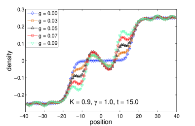
Figure 1: (Color online) Density at time $t$=$15$ after the quench for $K$=$0.9$, $\gamma$=$1$ and several different $g$.

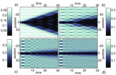
Figure 2: (Color online) Contour plots for the magnitude of the density for $K$=$0.9$, $\gamma$=$1$ and for values of $g$ a). g$=$0.05, b). g$=$0.2, c). g$=$0.6 and d). g$=$1.0. The density at $t$=$0$ is $\rho(x)$=$(1/4)\tanh{(x/3)}$.

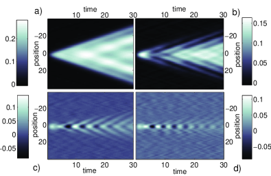
Figure 3: (Color online) Contour plots for the -(current) for $K$=$0.9$, $\gamma$=$1$ and for values of $g$ a). g$=$0.05, b). g$=$0.2, c). g$=$0.6 and d). g$=$1.0. The density at $t$=$0$ is $\rho(x)$=$(1/4)\tanh{(x/3)}$

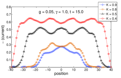
Figure 4: (Color online) The current at $t$=$15$ for $g$=$0.05$, $\gamma$=$1$ and different $K$.

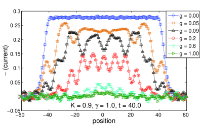
Figure 5: (Color online) The current at $t$=$40\,$ for $K$=$0.9,\gamma$=$1\,$ and different $g$.

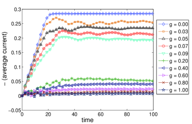
Figure 6: (Color online) Time evolution of the current after spatially averaging over a strip of width $\delta x=40$ centered at $x=0$.

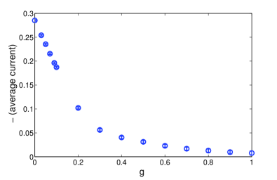
Figure 7: (Color online) Dependence of the steady-state average current on interaction $g$ for $\gamma=1$ and $K=0.9$.

II Time-evolution using the Truncated Wigner Approximation

We start with an initial state which is the ground state of the Luttinger liquid,

$$H_{i}= \frac{v_{F}}{2\pi}\int dx\left[\left(\partial_{x}\theta(x)\right)^{2}+\left(\partial_{x}\phi(x)\right)^{2}\right.$$ (1)

$$\left.+\frac{2}{v_{F}}h(x)\partial_{x}\phi(x)\right]$$

where in terms of bosonic creation and annihilation operators $b_{p},b_{p}^{\dagger}$ Giamarchi ,

$$\phi(x) = -\frac{i\pi}{L}\sum_{p\neq 0}\left(\frac{L|p|}{2\pi}\right)^{1/2}\frac{1}{p}e^{-\alpha|p|/2-ipx}\left(b_{p}^{\dagger}+b_{-p}\right)$$ (2)

$$\theta(x) = \frac{i\pi}{L}\sum_{p\neq 0}\left(\frac{L|p|}{2\pi}\right)^{1/2}\frac{1}{|p|}e^{-\alpha|p|/2-ipx}\left(b_{p}^{\dagger}-b_{-p}\right)$$ (3)

and $\left[\phi(x),\frac{1}{\pi}\partial_{y}\theta(y)\right]=i\delta(x-y)$. Above, $v_{F}$ is the Fermi velocity or the velocity of the bosons, $\alpha$ a short-distance cut-off, $p$ the momentum, $L$ the length of the system, and $h(x)$ is an external chemical-potential which couples to the density $\rho(x)$=$-\frac{1}{\pi}\partial_{x}\phi(x)$. In the ground state of $H_{i}$ the density simply follows the external field $\langle\rho(x)\rangle$=$\frac{1}{\pi v_{F}}h(x)$. We choose $h(x)$=$h_{0}\tanh{(x/\xi)}$ so that the initial density is a domain wall of width $\xi$. We study the case where at time $t$=$0$ the external field $h(x)$ is switched off. At the same time an optical-lattice is suddenly switched on which may be accompanied by an change in the interaction between bosons. Thus the time evolution for $t>0$ is due to the quantum sine-Gordon model,

$$H_{f}= \frac{u}{2\pi}\int dx\left[K\left(\partial_{x}\theta(x)\right)^{2}+\frac{1}{K}\left(\partial_{x}\phi(x)\right)^{2}\right]$$ (4)

$$-g\int dx\cos\left(\gamma\phi(x)\right)$$

Here $u$=$v_{F}/K$, $K$ being the Luttinger parameter and $g$ the strength of the back-scattering interaction arising due to a periodic potential. The ground state of $H_{f}$ has two well known phases, Giamarchi the localized (gapped) phase characterized by $\langle\phi\rangle\neq 0$, and a delocalized (gapless) phase. The periodic potential is a relevant parameter for $2-\frac{\gamma^{2}K}{4}>0$, implying that the ground state has a gap for infinitesimally small $g$. On the other hand for $2-\frac{\gamma^{2}K}{4}<0$, a localized phase arises only for back-scattering strengths larger than a critical value ($g>g_{c}$). We will study quenched dynamics for parameters that are such that $g$ is a relevant perturbation in equilibrium. Note that the initial domain wall state is not an exact eigen-state of $H_{f}$. Neither is it related to the classical solitonic solution of the QSG model since the latter is a domain wall in the $\phi$ field, Rajaraman while our initial state is a domain wall in $\partial_{x}\phi$.

When $g$=$0$, the time evolution of the system can be solved exactly. Lancaster10a For this case an initial density inhomogeneity shows typical light-cone dynamics Calabrese by spreading out ballistically in either direction with the velocity $u$, i.e., $\rho(x,t)$=$\frac{1}{2\pi v_{F}}\left[h(x+ut)+h(x-ut)\right]$. Since the system is closed, the energy is conserved. However during the course of the time-evolution, the energy density is transferred from the density to the current, the latter having the form

$$j(x,t) = \frac{1}{\pi}\frac{\partial\theta}{\partial x}$$ (5)

$$= \frac{1}{2\pi uK^{2}}\left[h(x-ut)-h(x+ut)\right]$$ (6)

In particular for $h(x)$=$h_{0}\tanh(x/\xi)$, the energy density at $t$=$0$ is ${\cal E}$=$\frac{u\pi}{2K}\langle\rho(x)\rangle^{2}\simeq h_{0}^{2}/(2\pi uK^{3})$, while at long times, and for positions within the light-cone ($ut>|x|$ ) the energy density is ${\cal E}$=$\frac{u\pi K}{2}j^{2}$ where $j$=$-h_{0}/(\pi uK^{2})$.

Note that while any initial density profile will give rise to transient currents, the special feature of a domain wall density profile is that for a system of infinite length, the steady state behavior is characterized by a net current flow. In particular for any finite time the current flows across a length $|x|=ut$ of the wire connecting the regions of high and low densities $\pm\rho_{0}=\pm h_{0}/(\pi v_{F})$ at the two ends.

We now explore how the time-evolution of the density, and the long time behavior of the current and two-point correlation functions is influenced by a back-scattering interaction ($g\neq 0$). The results are obtained using TWA which involves solving the classical equations of motion with initial conditions weighted by the Wigner distribution function of the initial state. Thus TWA is exact when $g$=$0$ while the effect of $g$ is the leading correction in powers of $\hbar$. Polkovreview Since $H_{i}$ is quadratic in the fields, it can be diagonalized by a simple shift, i.e., $H_{i}$=$\sum_{p\neq 0}v_{F}|p|a_{p}^{\dagger}a_{p}$, where $b_{p}$=$a_{p}+h_{p}/(v_{F}\sqrt{2\pi|p|L})$, $h_{p}$ being the Fourier transform of $h(x)$. The initial Wigner distribution function for the $a_{p}$ fields are Gaussian and are accessed by a Monte-Carlo sampling. This is followed by a Fourier transform defined in Eqns. 2 and 3 which gives the $\phi$ and $\theta$ fields at the initial time $t$=$0$. The classical equations of motion are then solved on a lattice up to a time $t$. All the data sets presented here are accompanied with error bars associated with the Monte-Carlo averaging. Lengths will be measured in units of the lattice spacing $a$ which is also set equal to the short-distance cut-off $\alpha$. Energy scales will be in units of $v_{F}/a$. The results will be presented for $h_{0}$=$\pi/4$ and an initial domain wall of width $\xi$=$3$.

II.1 Time evolution of the density

Fig. 1 shows the density at a time $t$=$15$ after the quench for $K$=$0.9$, $\gamma$=$1$ and several different $g$. The domain wall is found to broaden with time with a velocity which is reduced from the velocity of expansion $u$=$v_{F}/K$ when $g=0$. Moreover, unlike purely ballistic motion, the shape of the domain wall changes during the time-evolution. The behavior of the density is clearer in the contour plots in Fig. 2. For small $g$, the time-evolution shows a light-cone behavior along with the appearance of spatial oscillations within the light-cone. The amplitude of the oscillations increase with $g$, while the wavelength of the oscillations is set by $\rho_{0}$. Increasing $g$ gradually blurs the light-cone, and eventually for very large $g$ the domain wall mass becomes so large that it hardly moves during the times calculated here.

II.2 Time evolution of the current

The current behaves in a manner complementary to the density and consistent with the continuity equation. Fig. 3 shows contour plots for the current for parameters that are identical to that for the density shown in Fig. 2. The current, like the density, fluctuates in space and time, but on an average reaches a non-zero steady state within the light cone for $g$ values that are not too large. Fig. 4 shows the current at time $t$=$15$ for a given $g$ and different $K$. As $K$ decreases, the current increases as one expects from the analytic result for $g$=$0$. Fig. 5 shows how the current behaves for a fixed $K$ and different $g$. Increasing $g$ not only reduces the overall velocity of expansion, but also reduces the magnitude of the current. Fig. 6 shows how the current spatially averaged over a strip of width $40$ centered at the origin evolves in time. There is a clear appearance of a current carrying steady state whose magnitude decreases with $g$. Note that the spatial averaging under-estimates the time required to reach steady state as it under-estimates the amount of current for $ut\leq 20$.

The dependence of the steady state current on $g$ is plotted in Fig. 7 after time-averaging the current in Fig. 6 over a time window $t=40-100$ in order to eliminate the temporal fluctuations. The steady state current is found to decrease linearly with $g$ for $g\ll 1$. Note that when $g\neq 0$, the current does not commute with $H_{f}$. Yet the system reaches a current carrying steady state. This is due to the fact that the QSG model has a large number of other conserved quantities, some of which have a nonzero overlap with the current operator, thus preventing the current to decay to zero. The lack of decay of an initial current carrying state is also the origin of an infinite conductivity in many integrable systems. Giamarchi It was argued in Ref. Rosch00, that at least two different non-commuting Umpklapp processes are needed to violate conservation laws sufficiently so as to render the conductivity finite and thus cause the current to decay to zero.

II.3 Steady-state correlation functions

In this subsection we will study the following two equal time two-point correlation functions,

$$C_{\theta\theta}(xt;yt) = \langle e^{i\theta(x,t)}e^{-i\theta(y,t)}\rangle$$ (7)

$$C_{\phi\phi}(xt;yt) = \langle e^{i\phi(x,t)}e^{-i\phi(y,t)}\rangle$$ (8)

These are found to reach a nonequilibrium steady state for a time $ut>|x|,|y|$, i.e. for observation points that are within the light-cone. The result for $C_{\theta\theta}$ for $K$=$0.9$ and different $g$ is plotted in Fig. 8. The TWA result for $g$=$0$ is in agreement with the analytic result Lancaster10a $C_{\theta\theta}(x,y;ut>|x|,|y|)$=$\exp\left[ih_{0}(y-x)/(v_{F}K)\right]\left(\alpha/\mid x-y\mid\right)^{(1+K^{-2})/4}$. Thus when $g$=$0$, the correlation function decays as a power-law with a slightly larger exponent than in equilibrium (the latter being $C^{eq}_{\theta\theta}(x,y)$=$\left(\alpha/\mid x-y\mid\right)^{1/(2K)}$). Moreover $C_{\theta\theta}$ shows oscillations at wavelength $\lambda$=$\frac{2\pi v_{F}K}{h_{0}}$=$2/j$, $j$ being the steady-state current within the light cone. Note that the results for $h_{0}=0$ were obtained previously in Ref. Cazalilla06, where the authors studied an interaction quench from a homogeneous initial state. The physical reason for the spatial oscillations when $h_{0}\neq 0$ is the dephasing of the variable canonically conjugate to the density as the domain wall broadens. This implies a dephasing of transverse spin components in the $XX$ spin chain resulting in a spin-wave pattern at wavelength $\lambda$. Lancaster10a For a system of hard-core bosons, oscillations in $C_{\theta\theta}$ has the physical interpretation of the appearance of quasi-condensates at wave-vector $k$=$2\pi/\lambda$. Rigolqc

The TWA results presented here show that these effects can persist even in the presence of a back-scattering interaction, at least within the continuum model. In particular Fig. 8 shows that when $g\neq 0$, $C_{\theta\theta}$ retains the spatially oscillating form albeit at a wavelength that increases with increasing $g$. Just as for $g$=$0$, one expects the current to set the wavelength of the oscillations. To check this Figs. 9 and 10 show a comparison between $C_{\theta\theta}(xt,yt)$ and $C_{\theta\theta}(h_{0}$=$0)(xt,yt)\cos(\pi j(x-y))$ where $C_{\theta\theta}(h_{0}$=$0)(xt,yt)$ is the correlation function at long times after a homogeneous quench from $H_{i}$ to $H_{f}$ ($h_{0}$=$0$ in $H_{i}$), while $j$ is the spatially averaged steady-state current in Fig. 7. The agreement is found to be good at least for small $g$. The second effect of $g$ on $C_{\theta\theta}$ is to give rise to a faster decay in position. This decay also becomes faster for a given $g$ and on decreasing $K$ (not shown here) which takes the system deeper into the gapped phase of the QSG model.

Fig. 11 shows the behavior of $C_{\phi\phi}$ correlation function after it has reached a steady state. The result for $g$=$0$ is Cazalilla06 ; Lancaster10a $C_{\phi\phi}(x,y;ut>|x|,|y|)$=$\left(\alpha/\mid x-y\mid\right)^{(1+K^{2})/4}$ which is also characterized by a slightly faster power-law decay than in equilibrium (the latter being $C^{eq}_{\phi\phi}(x,y)$=$\left(\alpha/\mid x-y\mid\right)^{K/2}$). Further unlike $C_{\theta\theta}$, $C_{\phi\phi}$ has no memory of the initial spatial inhomogeneity for $g=0$. However this is no longer the case for nonzero $g$. Fig. 11 shows that for small $g$, $C_{\phi\phi}$ can also show spatial oscillations. Moreover, there is no appearance of long-range order until $g$ is ${\cal O}(1)$, where the appearance of the Ising gap corresponds to a nonzero asymptotic behavior of the two-point correlation function. It is also consistent that the appearance of the gap in $C_{\phi\phi}$ coincides with the value of $g$ for which the domain wall is almost static in Fig. 2.

In equilibrium, the $\cos\gamma\phi$ interaction is a relevant perturbation for $2>\gamma^{2}K/4$. Giamarchi Thus the $H_{f}$ parameters considered here are those for which the ground state is the gapped Ising phase for $g$ of any strength. Yet there is no signature of the gap in the quenched dynamics for $g\ll 1$. For this case the domain wall motion is ballistic, and the $C_{\theta\theta}$ correlations persist over longer distances than in the gapped Ising phase. Similar observations have also been made in the study of an interaction quench both in the bose-Hubbard model Kollath08 and for a system of interacting fermions manmana where it was found that the system continued to show light-cone dynamics and gapless behavior for parameters that correspond to the equilibrium gapped phase.

The time-evolution of the density and current in the XXZ chain for an initial domain wall state was studied in Ref. tdmrg1, employing TDMRG. There it was found that while a current persists within the gapless phase, it decayed to zero in the gapped phase. This result is different from what we find here where the current persists in the gapped phase as long as $g$ is not too large. There could be two reasons for this difference. Firstly the parameters $\gamma$, $g$ and $K$ that we use here, do not correspond to the parameters of the XXZ chain. Secondly, it is possible that the irrelevant operators that are not retained in the continuum model modify the long-time behavior, even though this was not found to be the case at the exactly solvable XX point ($J_{z}=0$, $K=1,g=0$). Lancaster10a

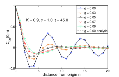
Figure 8: (Color online) The equal time $C_{\theta\theta}(0t;nt)$ correlation function at $t$=$45$ for $K$=$0.9$, $\gamma$=$1$ and different $g$.

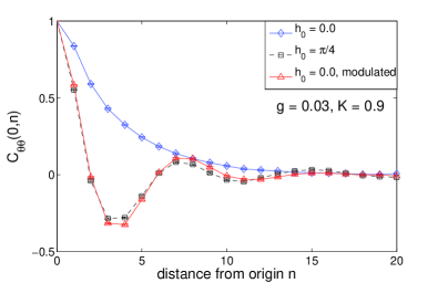
Figure 9: (Color online) The equal time $C_{\theta\theta}(0t;nt)$ correlation function compared with correlation function for a homogeneous quench ($h_{0}$=$0$) and modulated by $\cos(\pi jn)$ for $t$=$45$ and $g$=$0.03$, $K$=$0.9$, $\gamma$=$1$.

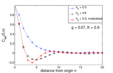
Figure 10: (Color online) The equal time $C_{\theta\theta}(0t;nt)$ correlation function compared with correlation function for a homogeneous quench ($h_{0}$=$0$) and modulated by $\cos(\pi jn)$ for $t=45$,$g$=$0.07$, $K$=$0.9$, $\gamma$=$1$.

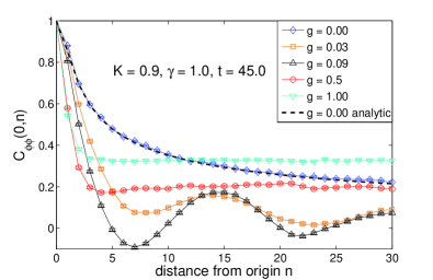
Figure 11: (Color online) The equal time $C_{\phi\phi}(0t;nt)$ correlation function at $t$=$45$ and for $K$=$0.9$, $\gamma$=$1$ and different $g$.

III Quantum corrections to TWA

An important question concerns the validity of TWA. It was shown in Ref. Polkovreview, that in writing the time-evolution of an interacting system as a Keldysh path integral, TWA is the leading correction in powers of $\hbar$. One may therefore check its validity by expanding the path integral in higher powers of $\hbar$, and identify when these contributions become significant. We evaluate the first quantum correction along the lines of Ref. Polkovreview, . Below we briefly outline the approach.

The expectation value of an observable $\hat{O}({\bf x},{\bf p},t)$ to leading order beyond TWA is Polkovreview

$$\left\langle\hat{O}({\bf x},{\bf p},t)\right\rangle\approx\int d{\bf x}_{0}d{\bf p}_{0}W_{0}({\bf x}_{0},{\bf p}_{0})$$

$$\left[1-\int_{0}^{t}d\tau\frac{\hbar^{2}}{3!2!i^{2}}\frac{\partial^{3}V}{\partial{\bf x}(\tau)^{3}}\frac{\partial^{3}}{\partial{\bf p}^{3}}\right]O_{W}({\bf x},{\bf p},t)$$ (9)

where $W_{0}({\bf x}_{0},{\bf p}_{0})\,$ is the initial Wigner distribution, and $O_{W}({\bf x},{\bf p},t)=\int d{\bf y}\left\langle{\bf x}-{\bf y}/2\right|\hat{O}({\bf x},{\bf p},t)\left|{\bf x}+{\bf y}/2\right\rangle e^{i{\bf p}\cdot{\bf y}/\hbar}\,$ is the Weyl symbol of the operator $\hat{O}$. In the QSG model, ${\bf x}\rightarrow\phi(x)$, ${\bf p}\rightarrow\Pi(x)\equiv\frac{1}{\pi}\partial_{x}\theta(x)$, and $\int d{\bf x}d{\bf p}\rightarrow\int\mathcal{D}\phi(x)\mathcal{D}\Pi(x)$. In Ref. Polkovreview, the author implemented this correction by allowing a stochastic quantum jump in the momentum variable during the time evolution. This is done as follows: for each Monte Carlo step, we choose a set of initial conditions, weighted by the initial Wigner distribution, in accordance with TWA. For each set of initial conditions, we select a random position, $x_{n}$, and a random time, $\tau$. During the classical evolution, the field $\Pi_{n}(t)=\Pi(x_{n},t)$ is given a quantum kick at time $\tau\,$ by shifting $\Pi_{n}(\tau)\rightarrow\Pi_{n}(\tau)+\xi(\Delta\tau)^{1/3}$, where $\xi\,$ is a random weight chosen from a Gaussian distribution of zero mean and unit variance, and $\Delta\tau\,$ is a small time interval. Here, we take $\Delta\tau\,$ equal to the integration time step size, $\Delta t$. This process of sampling $\tau$, $x_{n}$, and $\xi$ is repeated for a given set of initial conditions. Thus the quantum correction to TWA is Polkovreview

$$\left\langle-\frac{tNg\gamma^{3}}{8}\sin[\gamma\phi_{n}(\tau)]\left(\xi^{3}/3-\xi\right)\hat{O}(\phi,\Pi,t)\right\rangle,$$ (10)

where $N\,$ is the number of spatial points.

The results for the first quantum correction for $\gamma$=$1$ and $\gamma$=$2$ are shown in Fig. 12 and Fig. 13 respectively. As expected, the larger the coefficient $\gamma$, the larger the quantum fluctuations in the $\phi$ field, causing TWA to break down sooner. We find TWA to work very well for $\gamma$=$1$ up to times $t=15$. On the other hand, for the same times, the quantum corrections for $\gamma$=$2$ are significant.

It is also important to understand whether the steady-state current is a result of the truncation scheme. To check this we plot the current evaluated from TWA along with the first quantum correction in Fig. 14 for $\gamma=1$ and $K=0.9$. The current is now spatially averaged over the non-interacting light-cone $|x|<ut$. The quantum correction is found to enhance the current. This is expected on the grounds that TWA underestimates the quantum fluctuations, and therefore underestimates the extent of gapless behavior in the dynamics.

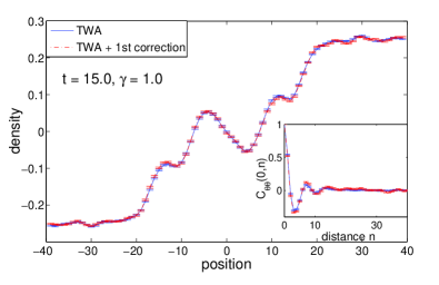
Figure 12: (Color online) TWA and first quantum correction for the density (main panel) and equal time $C_{\theta\theta}$ correlation function (inset) for $K$=$0.9,g$=$0.05,\gamma$=$1$ and $t$=$15$.

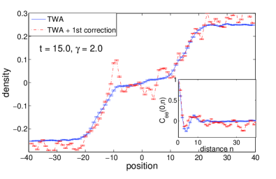
Figure 13: (Color online) TWA and first quantum correction for the density (main panel) and equal time $C_{\theta\theta}$ correlation function (inset) for $K$=$0.9,g$=$0.05,\gamma$=$2$ and $t$=$15$.

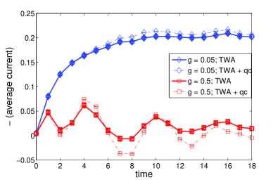
Figure 14: (Color online) TWA and first quantum correction to the current spatially averaged over the light-cone $ut$ for $K$=$0.9$ and $\gamma$=$1$ and several different $g$.

IV Quenched dynamics at the Luther-Emery point for an initial current carrying state

The main result of TWA was that a current carrying state can persist even in the gapped phase of a model. In this section we will explore this physics at the Luther-Emery point of the QSG model. In particular we will study how an initial current carrying state evolves in time when the back-scattering interaction is suddenly switched on. We will also explore the long time behavior of two point correlation functions.

The Luther-Emery point is a special point of the QSG model where the problem is rendered quadratic after refermionization in terms of left and right moving fermions $\psi_{L,R}$. Giamarchi To see this, we rescale the fields in Eqn. (4) as $\phi^{\prime}=\gamma\phi/2\,$ and $\theta^{\prime}=2\theta/\gamma$. Further if $K=4/\gamma^{2}$, then $H_{f}$ may be written as

$$H_{f}^{\prime} = -iu\int dx\left[\psi_{R}^{\dagger}(x)\partial_{x}\psi_{R}(x)-\psi_{L}^{\dagger}(x)\partial_{x}\psi_{L}(x)\right]$$ (11)

$$+ m\int dx\left[\psi_{R}^{\dagger}(x)\psi_{L}(x)+\psi_{L}^{\dagger}(x)\psi_{R}(x)\right]$$

where $m=g\pi\alpha$ and

$$\psi_{R}(x) = \frac{\eta_{R}}{\sqrt{2\pi\alpha}}e^{-i[\phi^{\prime}(x)-\theta^{\prime}(x)]},$$ (12)

$$\psi_{L}(x) = \frac{\eta_{L}}{\sqrt{2\pi\alpha}}e^{i[\phi^{\prime}(x)+\theta^{\prime}(x)]},$$ (13)

$\eta_{R,L}\,$ are Klein factors to ensure the correct anticommutation relations among the fermions.

We construct an initial current carrying state which is the ground state of the Hamiltonian

$$H_{i}^{\prime}= -iu\int dx\left[\psi_{R}^{\dagger}(x)(\partial_{x}-i\frac{\mu}{u})\psi_{R}(x)\right.$$ (14)

$$\left.-\psi_{L}^{\dagger}(x)(\partial_{x}-i\frac{\mu}{u})\psi_{L}(x)\right]$$

where $2\mu$ is the chemical potential difference between right and left movers. We then study the time-evolution of this state for $t>0$ due to the Hamiltonian $H_{f}^{\prime}$ (Eq. 11). This Hamiltonian has a back-scattering interaction of strength $m$, and no applied chemical potential difference between right and left movers ($\mu=0$).

Defining $\psi_{R/L}(x)=\int\frac{dk}{2\pi}e^{ikx}\psi_{R/L}(k)$, the initial state is characterized by the occupations

$$\langle\psi_{R}^{\dagger}(k)\psi_{R}(k)\rangle = \theta(-uk+\mu)$$ (15)

$$\langle\psi_{L}^{\dagger}(k)\psi_{L}(k)\rangle = \theta(uk-\mu)$$ (16)

The current is defined as

$$j(x)=u\left[\psi_{R}^{\dagger}(x)\psi_{R}(x)-\psi_{L}^{\dagger}(x)\psi_{L}(x)\right]$$ (17)

Thus the initial state is characterized by a current density

$$j_{0}=\mu/\pi$$ (18)

Since the theory is quadratic, the time-evolution can be studied in terms of

$$\psi_{R}(k,t) = \psi_{R}(k)f(k,t)+\psi_{L}(k)g(k,t)$$ (19)

$$\psi_{L}(k,t) = \psi_{L}(k)f^{*}(k,t)+\psi_{R}(k)g(k,t)$$ (20)

where $f(k,t)=\cos(\omega_{k}t)-i\sin(\omega_{k}t)\cos(2\theta_{k}),g(k,t)=-i\sin(\omega_{k}t)\sin{2\theta_{k}}$, $\omega_{k}$=$\sqrt{m^{2}+u^{2}k^{2}},\tan(2\theta_{k})$=$m/(uk)$.

Using the above it is straightforward to work out the current at long times after the quench. The current reaches a steady state

$$j=j_{0}-(m/\pi)\tan^{-1}\left(j_{0}\pi/m\right)$$ (21)

Note that this result is very similar to that obtained by TWA (Fig. 7) and predicts that the steady state current decays linearly with $m$ for $m\ll j_{0}$, while it decays as $1/m^{2}$ for large $m$. The persistence of an initial current carrying state even in the gapped phase of a Hamiltonian was also found in Ref. Klich, . Moreover in agreement with Ref. Klich, we find that the steady state current in the limit of very small initial current $j_{0}\ll m$ is found to scale as the cubic power of the initial current $j\propto j_{0}^{3}$.

We now turn to the evaluation of the steady-state gap and two point correlation functions. In terms of bosonic variables $\phi^{\prime}=\gamma\phi/2$ and $\theta^{\prime}=2\theta/\gamma$, the gap is

$$\langle e^{2i\phi^{\prime}(x,t)}\rangle=-\langle\psi_{R}^{\dagger}(x)\psi_{L}(x)\rangle$$ (22)

while the basic two-point correlation functions are

$$C_{\phi^{\prime}\phi^{\prime}}(x,t) = \langle e^{2i\phi^{\prime}(x,t)}e^{-2i\phi^{\prime}(0,t)}\rangle$$ (23)

$$= \langle\psi_{R}^{\dagger}(xt)\psi_{L}(xt)\psi_{L}^{\dagger}(0t)\psi_{R}(0t)\rangle$$

$$C_{\theta^{\prime}\theta^{\prime}}(x,t) = \langle e^{-2i\theta^{\prime}(x,t)}e^{2i\theta^{\prime}(0,t)}\rangle$$ (24)

$$= \langle\psi_{R}^{\dagger}(xt)\psi_{L}^{\dagger}(xt)\psi_{L}(0t)\psi_{R}(0t)\rangle$$

For long times after the quench we find

$$\langle e^{2i\phi^{\prime}(x,t)}\rangle=\frac{mu}{4\pi}\ln\left[\frac{u^{2}/\alpha^{2}}{m^{2}+\pi^{2}j_{0}^{2}}\right]=A(\alpha,m,j_{0})$$ (25)

where $\alpha$ is a short-distance cut-off. Thus the steady-state gap depends on the initial current $j_{0}$.

The two point correlations at long times are

$$C_{\phi^{\prime}\phi^{\prime}}(x,t) = |A(\alpha,m,j_{0})|^{2}+|\frac{1}{2}\delta(x)+iI_{b}+I_{a}|^{2}$$ (26)

$$C_{\theta^{\prime}\theta^{\prime}}(x,t) = \left(\frac{1}{2}\delta(x)+iI_{b}+I_{a}\right)\left(\frac{1}{2}\delta(x)-iI_{b}-I_{a}\right)$$ (27)

$$- \left(I_{d}+iI_{c}\right)^{2}$$

where

$$I_{a} = \int_{0}^{\mu/u}\frac{dk}{2\pi}\cos(kx)\frac{u^{2}k^{2}}{m^{2}+u^{2}k^{2}}$$ (28)

$$I_{b} = \int_{\mu/u}^{\infty}\frac{dk}{2\pi}e^{-k\alpha}\sin{kx}\frac{u^{2}k^{2}}{m^{2}+u^{2}k^{2}}$$ (29)

$$I_{c} = \int_{0}^{\mu/u}\frac{dk}{2\pi}\sin(kx)\frac{muk}{m^{2}+u^{2}k^{2}}$$ (30)

$$I_{d} = \int_{\mu/u}^{\infty}e^{-k\alpha}\frac{dk}{2\pi}\cos{kx}\frac{muk}{m^{2}+u^{2}k^{2}}$$ (31)

For $j_{0}=0$ ($\mu=0$), $C_{\phi^{\prime}\phi^{\prime}}$ reduces to the expression derived in. Iucci For $j_{0}\neq 0$ and long distances $\mu x/u\gg 1,mx/u\gg 1$ we find,

$$C_{\phi^{\prime}\phi^{\prime}}(x,t)=|A(\alpha,m,j_{0})|^{2}+\frac{1}{x^{2}}\left(\frac{\pi^{2}j_{0}^{2}}{\pi^{2}j_{0}^{2}+m^{2}}\right)^{2}$$ (32)

Thus the correlations are found to decay very slowly (as $1/x^{2}$) in position to their long distance value of the square of the gap. This should be contrasted with the equilibrium result where the decay to the long distance value is exponential. Giamarchi It is also interesting to compare this result with that of an interaction quench from an initial state which is the ground state of $H_{i}^{\prime}(\mu=0)$. Iucci For this case the decay to the long distance value is a power law $\left(1/x^{6}\right)$, but with a larger exponent than found here for the current carrying state.

The expression for $C_{\theta^{\prime}\theta^{\prime}}$ at long times after the quench is

$$C_{\theta^{\prime}\theta^{\prime}}(x,t\rightarrow\infty)=\frac{1}{x^{2}}\left(\frac{\pi^{2}j_{0}^{2}}{m^{2}+\pi^{2}j_{0}^{2}}\right)e^{-2i\pi j_{0}x/u}$$ (33)

and shows a similar slow decay as $1/x^{2}$ in position (in contrast to an exponential decay in equilibrium). Moreover, the current flow imposes spatial oscillations at a wavelength which is determined by the current.

This quench at the Luther Emery point did not involve a change in the Luttinger parameter $K$. Significantly different physics can occur after a similar quench that also changes the value of $K$. In Ref. Foster10, , the authors showed that changing $K\,$ can lead to the existence of “super solitons” at the Luther Emery point, where initial density inhomogeneities spread out with amplitudes that grow in time.

V Conclusions

In summary, we have performed a detailed study of quenched dynamics in an interacting $1$D system prepared initially in a domain wall state. The model, being integrable, never thermalizes with the system reaching a nonequilibrium current carrying state which is robust even in the presence of moderate back-scattering interactions. The current has interesting consequences for the correlation functions, most notably the appearance of spatial oscillations in the $C_{\theta\theta}$ correlation function. Our predictions for the current can be tested experimentally using presently available one-dimensional optical lattice techniques. rev2008 ; Weld09
Acknowledgments: AM is particularly indebted to A. Rosch and T. Giamarchi for helpful discussions. This work was supported by NSF-DMR (Award No. 0705584, 1004589 for JL and AM, and 0705847 for EG).

References

- (1) A. Polkovnikov, K. Sengupta, A. Silva and M. Vengalattore, arXiv:1007.5331.
- (2) I. Bloch, J. Dalibard and W. Zwerger, Rev. Mod. Phys. 80, 885 (2008).
- (3) D. Gobert, C. Kollath, U. Schollwöck, and G. Schütz, Phys. Rev. E 71, 036102 (2005).
- (4) S. Langer, F. Heidrich-Meisner, J. Gemmer, I. P. McCulloch and U. Schollwöck, Phys. Rev. B 79, 214409 (2009).
- (5) P. Calabrese, C. Hagendorf and P. Le Doussal, J. Stat. Mech.: Theory Exp., P07013 (2008).
- (6) J. Mossel and J. S. Caux, New J. Phys. 12, 055028 (2010).
- (7) J. Mossel, G. Palacios and J. S. Caux, arXiv:1006.3741.
- (8) M. Rigol and A. Muramatsu, Phys. Rev. Lett. 93, 230404 (2004).
- (9) M. S. Foster, E. A. Yuzbashyan and B. L. Altshuler, Phys. Rev. Lett. 105, 135701 (2010).
- (10) T. Giamarchi, Quantum Physics in One Dimension (Oxford University Press, Oxford, 2004).
- (11) A. B. Zamolodchikov, Pis. Zh. Eksp. Teor. Fiz 25, 499 (1977).
- (12) A. Polkovnikov, Annals of Phys. 325, 1790 (2010).
- (13) D. Weld, P. Medley, H. Miyake, D. Hucul, D. E. Pritchard and W. Ketterle, Phys. Rev. Lett. 103, 245301 (2009).
- (14) A. Rosch and N. Andrei, Phys. Rev. Lett. 85, 1092 (2000).
- (15) X. Zotos, F. Naef and P. Prelovsek, Phys. Rev. B 55, 11029 (1997).
- (16) J. Lancaster and A. Mitra, Phys. Rev. E 81, 061134 (2010).
- (17) R. Rajaraman, Solitons and Instantons (North-Holland, Amsterdam, 1982).
- (18) P. Calabrese and J. Cardy, J. Stat. Mech.: Theory Exp. P04010 (2005); Phys. Rev. Lett. 96, 136801 (2006).
- (19) M. A. Cazalilla, Phys. Rev. Lett. 97, 156403 (2006); A. Iucci and M. A. Cazalilla, Phys. Rev. A 80, 063619 (2009).
- (20) A. M. Läuchli and C. Kollath, J. Stat. Mech., P05018 (2008).
- (21) S. R. Manmana, S. Wessel, R. M. Noack and A. Muramatsu, Phys. Rev. B 79, 155104 (2009).
- (22) I. Klich, C. Lannert and G. Refael, Phys. Rev. Lett. 99, 205303 (2007).
- (23) A. Iucci and M. A. Cazallila, New J. Phys. 12, 055019 (2010).