Phase separation of binary fluids with dynamic temperature

Abstract

Phase separation of binary fluids quenched by contact with cold external walls is considered. Navier-Stokes, convection-diffusion, and energy equations are solved by lattice Boltzmann method coupled with finite-difference schemes. At high viscosity, different morphologies are observed by varying the thermal diffusivity. In the range of thermal diffusivities with domains growing parallel to the walls, temperature and phase separation fronts propagate towards the inner of the system with power-law behavior. At low viscosity hydrodynamics favors rounded shapes, and complex patterns with different lengthscales appear. Off-symmetrical systems behave similarly but with more ordered configurations.

I Introduction

When in a multi-phase system initially in a mixed state the temperature is decreased to values corresponding to a coexisting region of the phase diagram, domains of ordered phases start to form and grow with time. The process is called phase separation and is relevant for a large variety of systems GUNTON . In most of the cases studied theoretically, the temperature or other control parameters are assumed not depending on time and space, but are instantaneously set to their final values for coexistence. This assumption, reasonable in many situations, typically gives rise to a self-similar growth behavior with a characteristic domain size following a time power-law BRAY . However, there are cases where the dynamics of the control parameter needs to be considered SAARLOS since it can greatly affect the morphology of domains. In binary alloys, for example, slow cooling is used to produce optimal sequences of alternate bands of different materials METAL . In polymeric mixtures the possibility of controlling the demixing morphology by appropriate thermal driving has been studied in Refs. KREKHOV ; YAMAMURA ; modulated patterns have been observed when a mixture is periodically brought above and below the critical point TANAKA . Other worth examples of complex pattern formation due to the dynamics of the control parameters occur in crystal growth LANGER , immersion-precipitation membranes CHENG , or in electrolyte diffusion in gels LIESEGANG ; ANTAL .

In this paper we study binary fluids quenched by contact with cold walls at temperatures below the critical value. The behavior of binary fluids in sudden quenches at homogeneous temperature is quite known BRAY ; YEOMANS . For symmetric composition, the typical interconnected pattern of spinodal decomposition is observed. In the system here considered, phase separation is expected to start close to the walls and develop in the inner of the system following the temperature evolution. The dynamics of this process and the role of the velocity field have not been explored too much, in spite of their relevance for many of the systems mentioned above.

Two-dimensional studies of diffusive binary systems with cold sharp fronts propagating at constant speed have shown the formation of structures aligned on a direction depending on the speed FURUKAWA ; ANTAL ; HANTZ ; WAGNERFOARD ; KREK2 . These results are also supported by theoretical analysis WAGNERFOARD ; KREK2 . Lamellar-like structures have been also found in numerical studies of two-dimensional off-symmetrical binary systems with the temperature following a fixed diffusive law BALL . In a model with the temperature dynamically coupled to the concentration field, point-like cold sources have been shown to give rise to ring structures of alternate phases ESPANOL . On the other hand, more usual morphologies have been found in cases with fixed thermal gradient JASNOW , while complex phenomena such as sequential phase-separation cascades have been observed when the control parameter is slowly homogeneously changed VOLLMER . The effects of full coupling between all thermo-hydrodynamic variables have been not considered sofar.

The paper is organized as follows. In the next section the theoretical model and the numerical method are illustrated. The dynamics of our system is described by mass, momentum, and energy equations with thermodynamics based on a free-energy functional including gradient terms. In Section III the results of our simulations are shown. We will explore the control parameter space by varying the viscosity and the thermal diffusivity. This will allow to analyze the differences with respect to the behavior of binary fluids in instantaneous quenching. The presentation will be focused on few cases typical for each regime. A final discussion will follow in Section IV.

II The model

We consider a binary mixture with dynamical variables $T,$v$,n,\varphi$ which are, respectively, the temperature, the velocity, the total density, and the order parameter field being the concentration difference. Equilibrium properties are encoded in the free-energy

$$F=\int(\psi(n,\varphi,T)+\frac{1}{2}M|{\bf\nabla}\varphi|^{2})d{\bf r}$$ (1)

where

$$\psi(n,\varphi,T)=e-k_{B}T[n\ln(n)-\frac{n+\varphi}{2}\ln(\frac{n+\varphi}{2})-\frac{n-\varphi}{2}\ln(\frac{n-\varphi}{2})]$$ (2)

with $e=nk_{B}T+\frac{\lambda n}{4}(1-\frac{\varphi^{2}}{n^{2}})$ being the bulk internal energy and the term in square brackets the mixing entropy. The gradient term in Eq. (1) is a combination of an internal energy gradient contribution proportional to $K$ and of an entropic term proportional to $-C$ ONUKI , hence $M=K+CT$. The system has a critical transition at $k_{B}T_{c}=\lambda/2$ and the order parameter in the separated phases takes the values $\varphi_{\pm}(T)=\pm\sqrt{3n^{2}(T_{c}/T-1)}$. The dynamical equations are given by DGM

$$\partial_{t}n=-\partial_{\alpha}(nv_{\alpha}),$$ (3)

$$\partial_{t}\varphi=-\partial_{\alpha}(\varphi v_{\alpha})-2\partial_{\alpha}J_{\alpha}^{d},$$ (4)

$$\partial_{t}(nv_{\beta})=-\partial_{\alpha}(nv_{\alpha}v_{\beta})-\partial_{\alpha}(\Pi_{\alpha\beta}-\sigma_{\alpha\beta}),$$ (5)

$$\partial_{t}\widehat{e}=-\partial_{\alpha}(\widehat{e}v_{\alpha})-(\Pi_{\alpha\beta}-\sigma_{\alpha\beta})\partial_{\alpha}v_{\beta}-\partial_{\alpha}J^{q}_{\alpha},$$ (6)

where ${\bf J}^{d}$ and ${\bf J}^{q}$ are the diffusion and heat currents, $\Pi_{\alpha\beta}$ is the reversible stress tensor, $\sigma_{\alpha\beta}=\eta(\partial_{\alpha}v_{\beta}+\partial_{\beta}v_{\alpha})+(\zeta-2\eta/d)\delta_{\alpha\beta}\partial_{\gamma}v_{\gamma}$ is the dissipative stress tensor with $\zeta,\eta$ being the bulk and shear viscosities, respectively, $d$ the space dimension, and $\widehat{{e}}=e+\frac{K}{2}|{\bf\nabla}\varphi|^{2}$ the total internal energy density also including gradient contributions. We have recently established the expressions for the pressure tensor $\Pi_{\alpha\beta}$ and chemical potential $\mu$ GONN following the approach of Ref. ONUKI . One finds

$$\Pi_{\alpha\beta}=\left(p-M\varphi\nabla^{2}\varphi-M{|{\bf\nabla}\varphi|^{2}}/2-T\varphi{\bf\nabla}\varphi\cdot{\bf\nabla}({M}/{T})\right)\delta_{\alpha\beta}+M\partial_{\alpha}\varphi\partial_{\beta}\varphi$$ (7)

where $p=-\psi+n\partial\psi/\partial n+\varphi\partial\psi/\partial\varphi$ and $\mu=\partial\psi/\partial\varphi|_{T}-T{\bf\nabla}\cdot[(M/T){\bf\nabla}\varphi]$. Finally, in order to completely set up the dynamical system, phenomenological expressions for the currents are needed. As usually, one takes ${\bf J}^{d}=-\mathcal{L}_{11}{\bf\nabla}({\mu}/{T})+\mathcal{L}_{12}{\bf\nabla}({1}/{T})$, ${\bf J}^{q}=-\mathcal{L}_{21}{\bf\nabla}({\mu}/{T})+\mathcal{L}_{22}{\bf\nabla}({1}/{T})$ where $\mathcal{L}_{\alpha\beta}$ is the positively defined matrix of kinetic coefficients with $\mathcal{L}_{11}=T\Gamma$ and $\mathcal{L}_{22}=T^{2}k$, $\Gamma$ and $k$ being the mobility and thermal diffusivity, respectively, assumed constant DGM .

In order to solve Eqs. (3-6) in $d=2$ we have developed a hybrid lattice Boltzmann method (LBM) lall ; xu ; maren ; STELLA where LBM LBM is used to simulate the continuity and Navier-Stokes equations (3) and (5) while finite-difference methods are implemented to solve the convection-diffusion and the energy equations (4) and (6). LBM has been widely used to study multi-phase/component fluids DUN and, in particular, hydrodynamic effects in phase ordering CATES . It is defined in terms of a set of distribution functions, $f_{i}({\bf r},t)$ with $i=0,1,...,8$, located in each site ${\bf r}$ at each time $t$ of a D2Q9 (2 space dimensions and 9 lattice velocities) lattice where sites are connected to first and second neighbors by lattice velocity vectors of modulus $|{\bf e}_{i}|=c$ ($i=1,...,4$) and $|{\bf e}_{i}|=\sqrt{2}c$ ($i=5,...,8$), respectively. The zero velocity vector ${\bf e}_{0}=0$ is also included. The lattice speed is $c=\Delta x/\Delta t$ where $\Delta x$ and $\Delta t$ are the lattice and time steps, respectively. The distribution functions evolve according to a single relaxation time Boltzmann equation bgk supplemented by a forcing term guo

$$f_{i}({\bf r}+{\bf e}_{i}\Delta t,t+\Delta t)-f_{i}({\bf r},t)=-\frac{\Delta t}{\tau}[f_{i}({\bf r},t)-f_{i}^{eq}({\bf r},t)]+\Delta tF_{i}({\bf r},t),$$ (8)

where $\tau$ is the relaxation parameter, $f_{i}^{eq}$ are the equilibrium distribution functions, and $F_{i}$ are the forcing terms to be properly determined.

The total density and the fluid momentum are given by the following relations

$$n=\sum_{i}f_{i},\hskip 36.98866ptn{\bf v}=\sum_{i}f_{i}{\bf e}_{i}+\frac{1}{2}{\bf F}\Delta t,$$ (9)

where ${\bf F}$ is the force density acting on the fluid. The $f_{i}^{eq}$ are expressed as a standard second order expansion in the fluid velocity ${\bf v}$ of the Maxwell-Boltzmann distribution functions qian . The forcing terms $F_{i}$ in Eq. (8) are expressed as a second order expansion in the lattice velocity vectors LADD . The continuity and the Navier-Stokes equations (3) and (5) can be recovered by using a Chapman-Enskog expansion when the $F_{i}$ are given by

$$F_{i}=\left(1-\frac{\Delta t}{2\tau}\right)\omega_{i}\left[\frac{{\bf e}_{i}-{\bf v}}{c^{2}_{s}}+\frac{{\bf e}_{i}\cdot{\bf v}}{c^{4}_{s}}{\bf e}_{i}\right]\cdot{\bf F}$$ (10)

with the force density ${\bf F}$ having components

$$F_{\alpha}=\partial_{\alpha}(nc_{s}^{2})-\partial_{\beta}\Pi_{\alpha\beta},$$ (11)

$c_{s}=c/\sqrt{3}$ being the speed of sound in the LBM, $\omega_{0}=4/9$, $\omega_{i}=1/9$ for $i=1,...,4$, and $\omega_{i}=1/36$ for $i=5,...,8$. We observe that in this formulation the pressure tensor is inserted as a body force in the lattice Boltzmann equations. From the Chapman-Enskog expansion it comes out that $\xi=\eta$ with

$$\eta=nc_{s}^{2}\Delta t\left(\frac{\tau}{\Delta t}-\frac{1}{2}\right).$$ (12)

On the other hand, a two-step finite difference scheme is used for the equations (4) and (6) (details on the implementation of Eq. (4) in the case of an isothermal LBM can be found in Ref. STELLA ). At walls, no-slip boundary conditions are adopted for the LBM PHYSA , the temperature is set to fixed values $T_{b}$ at the bottom wall and $T_{u}$ at the up wall, respectively, and neutral wetting for the concentration is adopted. This latter condition corresponds to impose ${\bf a}\cdot\nabla\varphi|_{walls}=0$ and ${\bf a}\cdot\nabla(\nabla^{2}\varphi)|_{walls}=0$, where ${\bf a}$ is an inward normal unit vector to the walls. These conditions together ensure ${\bf a}\cdot\nabla\mu|_{walls}=0$ so that the concentration gradient is parallel to the walls and there is no flux across the walls. We have found this algorithm stable in a wide range of temperatures, viscosities and thermal diffusivities. With respect to thermal LBM for non-ideal fluids SOFO where lattice Boltzmann equations are used to simulate the full set of macroscopic dynamical equations, the present model allows to reduce the number of lattice velocities thus speeding up the code and reducing the required memory STELLA .

III Results and discussion

In the following we will explore the parameter space keeping fixed the values of $K=0.003,C=0,k_{B}T_{c}=0.005,\Gamma=0.1$, and $\mathcal{L}_{12}=\mathcal{L}_{21}=0$. We will use lattices of size ranging from $256\times 256$ to $1024\times 1024$. We have considered different values of $\eta$ and $k$. Before focusing on the cases representative of the various regimes, we will list all the runs we did in terms of dimensionless numbers.

Common numbers used in hydrodynamics are the Reynolds and Peclet numbers $Re$ and $Pe$. They are defined as $Re=vL/\nu$, where $\nu=\eta/n$ is the kinematic viscosity, $Pe_{md}=vL/D$ for mass diffusion, where $D$ is the mass diffusion coefficient, and $Pe_{td}=vL/k$ for thermal diffusion. $L$ and $v$ are a typical length and velocity of the system. In phase separation $L$ can be identified with the average size of domains so that $Re$ and $Pe$ would depend on time (for a discussion see Ref. kendon ). It is therefore more convenient for our purposes to introduce the Schmidt and Prandtl numbers $Sc$ and $Pr$ defined as $Sc=\nu/D$ and $Pr=\nu/k$, where $D=|a|\Gamma$ with $a=(k_{B}T_{c}/n)(T/T_{c}-1)$ being the coefficient of the linear term in the chemical potential $\mu$ KREKHOV ; GONN . Here $T$ can be chosen as the value of the temperature at the walls. Table I contains a list of the runs we did, reported in terms of $Sc$ and $Pr$. It is also useful to evaluate the Mach number $Ma=|{\bf v}|_{max}/c_{s}$ where $|{\bf v}|_{max}$ is the maximum value of the fluid velocity during evolution. In all our simulations $Ma$ is always much smaller than $0.1$ (see in the following), and the fluid results practically incompressible, as checked, with $n\simeq 1$. For this reason we do not present in the paper any result about the time evolution of the total density $n$.

First, as a benchmark for our method, we consider the relaxation of a single interface profile with $k=10^{-2}$ and $\eta=0.167$ ($\tau=1$). This corresponds to a low viscosity regime as discussed in the following. We started the simulation with a sharp concentration step with values $\varphi_{-}(T_{b})$ and $\varphi_{+}(T_{u})$ and bulk temperature $T/T_{c}=0.8$ keeping fixed the temperatures $T_{b}/T_{c}=0.8,T_{u}/T_{c}=0.9$ at the bottom and up walls (Fig. 1 (a)). The system reaches a stationary state with constant temperature gradient and concentration profile as in Fig. 1 (b). The numerical values of concentrations in the two bulk phases are in very good agreement with the analytical expression for $\varphi_{\pm}(T({\bf r}))$ corresponding to the equilibrium values of $T({\bf r})$ shown in the related inset. This means that the concentration field $\varphi$ is in local equilibrium. The temperature of the up wall is then set to the same value of the temperature of the bottom wall (Fig. 1 (c)). Then, as it can be seen in Fig. 1 (d), the system equilibrates at constant temperature with the expected concentration profile. Spurious velocities are of order $10^{-9}$ and result completely negligible. The test shows that stationary states are well reproduced by our algorithm.

III.1 Diffusive regime

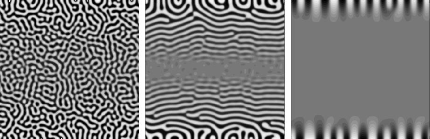
Figure 2: Typical configurations of the concentration field $\varphi$ for symmetric composition at very high viscosity ($\eta=6.5$) with $k=10^{-1},10^{-2},10^{-5}$ (from left to right) at times $t=12.5\times 10^{5};37.5\times 10^{5};300\times 10^{5}$, respectively, with lattice size $512\times 512$, and $T_{b}/T_{c}=T_{u}/T_{c}=0.8$.

We describe our results for phase separation. We first consider a case at very high viscosity with $\eta=6.5$ ($\tau=20$) and symmetric composition (Runs 1-8). Here the effects of the velocity field are negligible. We set $T_{b}/T_{c}=T_{u}/T_{c}=0.8$ and initial bulk temperature above $T_{c}$. As it can be seen in Fig. 2, for thermal diffusivities $k\geq 10^{-1}$, usual isotropic phase separation is observed. In the range $k=5\times 10^{-4}\div 5\times 10^{-2}$, in spite of the neutral wetting condition on the boundaries, domains in the bulk have interfaces preferentially parallel to thermal fronts. For smaller values of $k$ domains grow perpendicularly to the walls. These results agree with those of Refs. FURUKAWA ; WAGNERFOARD ; KREK2 in purely diffusive models where the same morphological sequence was found by decreasing the speed of cold fronts moving into a region with the mixed phase. However, also in absence of hydrodynamic effects, our case is different since the thermodynamics of the mixture is fully consistently treated and temperature fronts have no sharp imposed profile.

We will now concentrate on cases at intermediate thermal diffusivities where domains are parallel to the walls and propagation fronts can be traced. Concentration and temperature configurations at successive times for $k=10^{-2}$ (Run 4a) are shown in Fig. 3 and Fig. 4, respectively. In this case it is $Ma\simeq 5\times 10^{-5}$. The temperature fronts have typical diffusive profiles which slowly relax to the equilibrium value imposed on the boundaries. In order to be quantitative, we defined $y_{T}(t)$ as the distance from the wall where the temperature assumes a fixed value (we chose $T/T_{c}=0.88$) and measured this quantity in simulations with large rectangular lattices. The solution of the diffusion equation with initial temperature $T_{0}$ and fixed boundary value $T_{w}$ is $(T(y,t)-T_{w})/(T_{0}-T_{w})=erf{[y/(2\sqrt{kt})]}$ which implies $y_{T}/\sqrt{k}\sim\sqrt{t}$. In the inset of Fig. 5 it is shown, in simulations with different $k$, that $y_{T}$ follows the standard diffusion behavior. The time behavior of $y_{T}$ has been checked not depending on the specific value of the ratio $T/T_{c}$ in the range $[0.8,1.0]$; by considering a value of $T$ such that $T/T_{c}<1$ allows to track the position of the temperature front for a longer time interval.

One can also consider the behavior of the fronts limiting the regions with separated phases, clearly observable in the first three snapshots of Fig. 3. Their position can be defined as the distance $y_{\varphi}$ from the walls beyond which the condition $\nabla\varphi\simeq 0$ is verified everywhere. More precisely, we took $y_{\varphi}$ as the point beyond which $|\nabla\varphi|<C$ with $C=\sqrt{2}\times 0.01$; the value of $C$ is chosen to match the maximum value of the fluctuations of $|\nabla\varphi|$ in the initial disordered state, where $|\varphi|<0.01$. (In the last snapshot of Fig. 3 the two fronts propagating from up and down have come close each other and more usual phase separation occurs in the central region of the system.) We measured $y_{\varphi}$ on rectangular lattices for different $k$ and observed deviations from diffusive behavior (see Fig. 5). We found that $y_{\varphi}$ grows by power law with an exponent depending on $k$. Our fits give $y_{\varphi}\sim t^{0.66}$ for $k=10^{-2}$ and exponents closer to $1/2$ for smaller $k$. We analyzed for different $k$ possible variations of the typical values of fluid velocity but we did not find any. Therefore the change of the exponent of $y_{\varphi}$ cannot be attributed to the velocity field. Even if $y_{\varphi}$ moves faster than $y_{T}$ and at long times it results $y_{\varphi}>y_{T}$, we checked that the relation $y_{\varphi}<y_{T_{c}}$ is always verified so that phase separation always occurs for $T<T_{c}$. Since the phase separation is induced by the temperature change, one could have expected a similar behavior for $y_{\varphi}$ and $y_{T}$. The discrepancy could be related to the broad character of the temperature fronts which spreads the phase separated region. We also observed that the width of lamellar domains decreases at larger $k$, in agreement with Ref. WAGNERFOARD .

III.2 Hydrodynamic regime

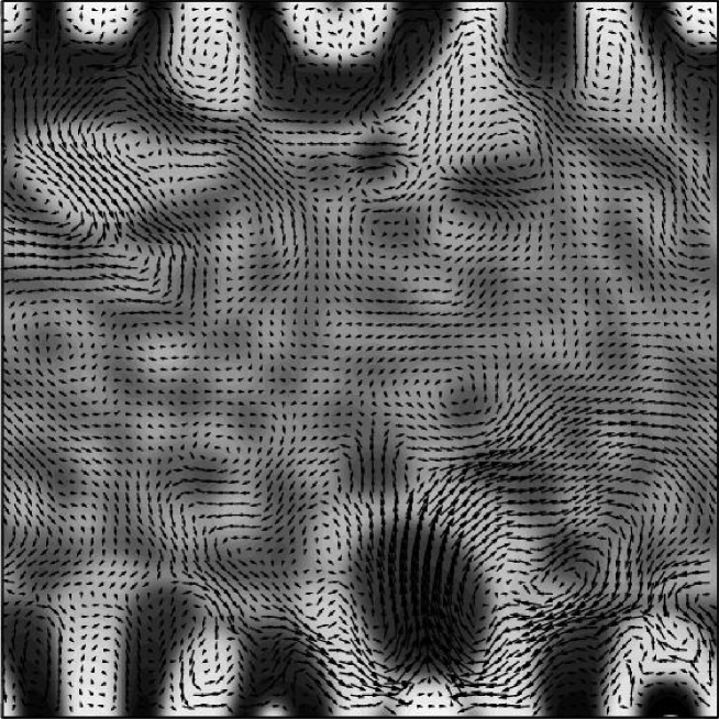
Figure 7: Configuration of concentration $\varphi$ for the case of Fig. 6 at time $t=11\times 10^{5}$ with superimposed the velocity field.

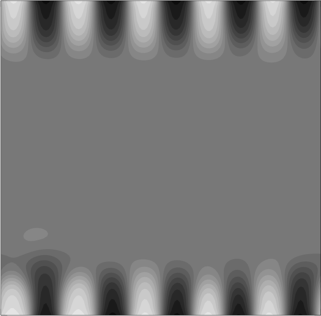
Figure 8: Configuration of concentration $\varphi$ at time $t=14\times 10^{5}$, low viscosity ($\eta=0.167$) as in Fig. 6, lattice size $128\times 128$, $T_{b}/T_{c}=T_{u}/T_{c}=0.8$, and $k=10^{-4}$.

At lower viscosities the evolution of morphology is very different in the range with intermediate values of thermal diffusivity. We will in particular illustrate in Fig. 6 the case with $\eta=0.167$ ($\tau=1$) and $k=10^{-2}$ (Runs 19), for which we found $Ma\simeq 5\times 10^{-4}$. This is the same thermal diffusivity of Fig. 3. At this viscosity hydrodynamics is relevant. Indeed, in instantaneous quenching at constant temperature and $\eta=0.167$ we observed the domain growth exponent to assume the inertial value $2/3$ (at odd with the diffusive high-viscosity value $1/3$ ) YEOMANS . The growth exponent was calculated by measuring the characteristic length defined by the inverse of the first momentum of the structure factor corb . The main effect due to hydrodynamics observable in Fig. 6 is that domains do not grow aligned with temperature fronts as it occurs for the same thermal diffusivity at high viscosity. Circular patterns are stabilized by the flow YEOMANS and an example is given in Fig. 7. A similar picture occurs for other values of $k$ here not reported (see Table I). On the other hand, the other thermal diffusivity regimes are less affected by hydrodynamics. When decreasing $k$, it is still possible to observe domains growing with interfaces normal to the walls as in the case at high viscosity (see Fig. 8 - Run 21b), while at larger $k$ (Run 18) phase separation occurs isotropically like in an instantaneous quenching.

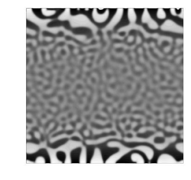
Figure 9: Configuration of concentration $\varphi$ at time $t=21\times 10^{5}$, intermediate viscosity ($\eta=2.167$), lattice size $512\times 512$, $T_{b}/T_{c}=T_{u}/T_{c}=0.8$, and $k=10^{-2}$.

The cases shown in Figs. 3 and 6 are typical of the high and low viscosity regimes. At intermediate values of $\eta$ one can observe features common to the two above cases (see Fig. 9 for $\eta=2.167$ - Run 11a). Concerning the behavior of $y_{T}(t)$, we could not find relevant differences by varying $\eta$ with respect to the case at high viscosity.

Another effect induced by hydrodynamics is the formation of structures in the inner part of the system at earlier times than in the case at high viscosity (compare Fig. 3 and Fig. 6). In the inner region we can observe the typical interconnected pattern of spinodal decomposition but with a characteristic length-scale different from that of domains close to the walls. However, while the structures close to the walls are in local equilibrium, that is $\varphi({\bf r})=\varphi_{\pm}(T({\bf r}))$, in the middle of the system the concentration field is such that $|\varphi|<\varphi_{+}(T({\bf r}))$. A temporal regime characterized by the presence of domains with two scales was found in systems of different size (from $256\times 256$ to $1024\times 1024$) and $k=10^{-3}\div 10^{-2}$. In order to characterize the two scales we analyzed the behavior of the structure factor. In Fig. 10 the spherically averaged structure factor is shown at two consecutive times for a system having the same parameters of Fig. 6 and size $L=512$. Two peaks are observable at each time that can be interpreted as related to the existence of two different length scales with one about twice longer than the other. The higher peak at smaller wave vector corresponds to the larger domains close to the walls while the other peak is related to the thinner domains in the inner of the system. At increasing times, the two peaks tend to merge. Due to this morphological evolution, in simulations at low viscosity, the position of the phase separation front $y_{\varphi}$ could be measured only for a short time interval making not possible to determine the power-law behavior.

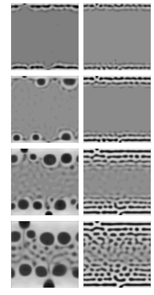
Figure 11: Configurations of concentration $\varphi$ for composition $55/45$ at times $t=4\times 10^{5};6\times 10^{5};11\times 10^{5};16\times 10^{5}$, low viscosity (left column) and very high viscosity (right column), lattice size $256\times 256$, $T_{b}/T_{c}=T_{u}/T_{c}=0.8$, and $k=10^{-2}$. Except for the composition, here the parameters are the same used in Figs. 6 and 3.

Finally, we show results for systems with asymmetric composition. In Fig. 11 the evolution of two systems only differing for the value of viscosity is shown. Lamellar patterns prevail at high viscosity while circular droplets dominate at low viscosity ($\eta=0.167$). In the latter case, again, two typical scales can be observed with thin tubes of materials connecting larger domains. The behavior of $y_{T}$ is similar to that of the symmetric case.

IV Conclusions

We have developed a numerical method for thermal binary fluids described by continuity, Navier-Stokes, convection-diffusion, and energy equations. We have studied quenching by contact with external walls, and we have shown how the pattern formation depends on thermal diffusivity, viscosity, and composition of the system. The evolution is very different from that observed in instantaneous homogeneous quenching. At high viscosity, different orientations of domains are possible. In an intermediate range of thermal diffusivities domains are parallel to the walls. The fronts limiting the regions with separated domains move towards the inner of the system with a power law behavior not always corresponding to that of the temperature fronts. At low viscosity, the velocity field favors more circular patterns, and domains are characterized by different length-scales close to the walls and in the inner of the system. Off-symmetrical mixtures give more ordered patterns.

We conclude with two remarks on possible future directions of work. The first one concerns the Soret effect, which corresponds to have a mass diffusion current induced by thermal gradients. This effect can become relevant in quenching very close to the critical point where the ratio $D_{T}/D$ becomes large KREKHOV . Here $D_{T}$ is the thermal (mass) diffusion coefficient ($D_{T}=\mathcal{L}_{12}/T^{2}$ in our notation) and $D$ is the mass diffusion coefficient defined at the beginning of Section III. In order to have a first idea on how the Soret effect can affect the pattern morphology, we considered a case with $D_{T}/D=20$ corresponding to the highest values for this ratio reported in literature KREKHOV . This would give $D_{T}=2\times 10^{-3}$, taking for $D$ the value used in the runs of Section III. We run simulations for this case. We observed, in the intermediate range of thermal diffusivity and at high viscosity, the tendency of the system to exhibit more ordered lamellar patterns (parallel to the walls). At higher thermal diffusivity isotropic phase separation is found as usually, while at very low thermal diffusivity ($k=10^{-4}$), parallel patterns are found instead of perpendicular patterns. At low viscosity (we tested the case corresponding to that of Fig. 6) hydrodynamics continues to favor domains with more circular shape. We run also simulations with $D_{T}=10^{-4}$, corresponding to a ratio $D_{T}/D\simeq 1$, without finding relevant differences with the respect to the case with $D_{T}=0$. We also observe that the behavior of $y_{\varphi}$ could depend on our choice for $\mathcal{L}_{12}$ and $\mathcal{L}_{21}$. A more comprehensive analysis of the Soret effect will be presented elsewhere.

Finally, the morphology could be still richer in three dimensions, also due to the existence of more hydrodynamic regimes BRAY , so that three-dimensional simulations would complete the picture given sofar.

Run	Size	$Sc$ ($\times 10^{3}$)	$Pr$	Symbol
1	512	65	12	I
2a, 2b	512, 256	65	66	I
3	512	65	129	Pa
4a, 4b	512, 256	65	651	Pa
5a, 5b	512, 256	65	1299	Pa
6	256	65	6500	Pa
7	512	65	65000	Pe
8	256	65	650000	Pe
9	256	21.7	22	I
10	256	21.7	43	I, Pa
11a, 11b	512, 256	21.7	217	I, Pa
12	256	21.7	2167	Pe
13	256	21.7	21667	Pe
14	256	8.3	8	I
15	256	8.3	83	I*
16	256	8.3	833	I*, Pe
17	256	8.3	8333	Pe
18	512	1.7	3	I
19a, 19b, 19c	1024, 512, 256	1.7	17	I*
20a, 20b	512, 256	1.7	167	I*
21a, 21b	512, 128	1.7	1667	Pe

Table 1: The first column indexes the simulation run, the second one is the linear size of the lattice, the third one is the Schmidt number ($Sc$), the fourth one is the Prandtl number ($Pr$). The last column is the symbol that identifies the kind of different observed patterns: I (isotropic morphology), Pa (domains parallel to the walls), Pe (domains perpendicular to the walls), I* (isotropic morphology with two lengthscales). The runs with two symbols exhibit patterns with common features to those corresponding to each symbol.

Figure 1: Concentration and temperature (inset) profiles for an interface relaxation (see the text for explanation).

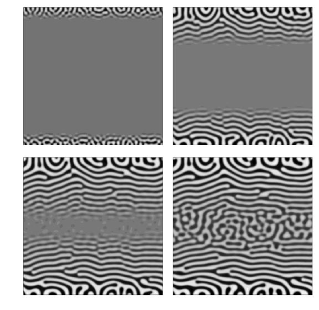
Figure 3: Configurations of concentration $\varphi$ for composition $50/50$ at times $t=7.5\times 10^{5};22.5\times 10^{5};37.5\times 10^{5};50\times 10^{5}$, at very high viscosity ($\eta=6.5$) with lattice size $512\times 512$, $T_{b}/T_{c}=T_{u}/T_{c}=0.8$, and $k=10^{-2}$.

Figure 4: Configurations of the ratio $T/T_{c}$ for the same case and at same times of Fig. 3. Coordinates on the $x$ and $y$ axes are in lattice units and both of them are in the range $[0,512]$.

Figure 5: Time behavior of $y_{\varphi}$ at $k=10^{-2}$ (empty symbols) and $10^{-3}$ (filled symbols) at very high viscosity with lattice size $128\times 2048$. The straight line is a guide to the eye and has slope $2/3$. Inset: Time behavior of $y_{T}/\sqrt{k}$ at $k=10^{-2}$ (empty symbols) and $10^{-3}$ (filled symbols). The straight line has slope $1/2$.

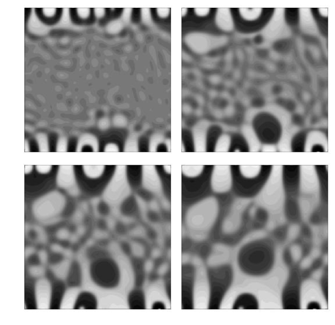
Figure 6: Configurations of concentration $\varphi$ for composition $50/50$ at times $t=8\times 10^{5};11\times 10^{5};13\times 10^{5};15\times 10^{5}$, low viscosity ($\eta=0.167$), lattice size $256\times 256$, $T_{b}/T_{c}=T_{u}/T_{c}=0.8$, and $k=10^{-2}$.

Figure 10: Spherically averaged structure factor $C(k)$ as a function of the wave vector modulus $k$ for a system with the same parameters of Fig. 6 and size $L=512$ at times $t=24\times 10^{5}$ (empty symbols) and $t=39\times 10^{5}$ (filled symbols), corresponding to the regime with two scales shown in Fig. 6.