Differential rotation of main-sequence dwarfs and its dynamo-efficiency

Abstract

A new version of a numerical model of stellar differential rotation based on mean-field hydrodynamics is presented and tested by computing the differential rotation of the Sun. The model is then applied to four individual stars including two moderate and two fast rotators to reproduce their observed differential rotation quite closely. A series of models for rapidly rotating ($P_{\mathrm{rot}}=1$ day) stars of different masses and compositions is generated. The effective temperature is found convenient to parameterize the differential rotation: variations with metallicity, that are quite pronounced when the differential rotation is considered as a function of the stellar mass, almost disappear in the dependence of differential rotation on temperature. The differential rotation increases steadily with surface temperature to exceed the largest differential rotation observed to date for the hottest F-stars we considered. This strong differential rotation is, however, found not to be efficient for dynamos when the efficiency is estimated with the standard $C_{\Omega}$-parameter of dynamo models. On the contrary, the small differential rotation of M-stars is the most dynamo-efficient. The meridional flow near the bottom of the convection zone is not small compared to the flow at the top in all our computations. The flow is distributed over the entire convection zone in slow rotators but retreats to the convection zone boundaries with increasing rotation rate, to consist of two near-boundary jets in rapid rotators. The implications of the change of the flow structure for stellar dynamos are briefly discussed.

1 Introduction

The theory of stellar differential rotation is mainly focused on the Sun where helioseismology provides all the possibilities for a detailed testing of computations. Applications to other stars are, however, tempting in view of the rapid development of asteroseismology (Christensen-Dalsgaard, 2008) that can eventually provide data on internal stellar rotation (Suárez et al., 2010). A knowledge of differential rotation is also considered as a key for stellar dynamos.

Until recently, precise measurements of differential rotation were mainly provided by Doppler imaging (Donati & Collier Cameron, 1997; Strassmeier, 2004; Barnes et al., 2005). This technique is most suitable for rapidly rotating stars (Donati, 1996). Young dwarfs with rotation periods $P_{\mathrm{rot}}\sim 1$ day present, however, difficulties for theory. Rapid rotators have thin boundary layers at the top and bottom of their convection zones (Durney, 1989; Kitchatinov & Rüdiger, 1999), which are difficult to resolve numerically. Almost no computations of differential rotation for rapid rotators were attempted.

The situation has changed recently. First, measurements of the differential rotation of two not too rapidly rotating, $P_{\mathrm{rot}}\sim 10$ days, main-sequence dwarfs were performed using high-precision photometry of the asteroseismological MOST mission (Croll et al., 2006; Walker et al., 2007). Second, a new mean-field code was developed that can resolve boundary layers in rapidly rotating stars; this code is used for the first time to produce the results of this paper. We first apply it to the Sun to check its ability to reproduce helioseismological inversions. Then, the differential rotation of the MOST-stars ($\epsilon$ Eri and $\kappa^{1}$ Ceti) are computed and compared with observations. We also compute the differential rotation of AB Dor and LQ Hya which probably have been the most frequent observational targets for Doppler imaging among dwarf stars (Donati & Collier Cameron, 1997; Collier Cameron & Donati, 2002; Donati, Collier Cameron & Petit, 2003; Kővári et al., 2004).

We further compute the dependence of differential rotation on the surface temperature for rapidly rotating stars. On an observational basis, the dependence has been studied by Barnes et al. (2005). The theoretical and observational results are quite similar. They both show a rapid increase of surface differential rotation with temperature. Reiners & Schmitt (2002, 2003) found that the rotation of F-stars can be strongly non-uniform. Recently Jeffers & Donati (2008) observed a large differential rotation with a pole-equator lap time slightly above 10 days on a rapidly rotating G0 dwarf. Our computations suggest that shallow convection zones of F-stars can possess even stronger differential rotation. This raises the question of whether the strong rotational shear implies over-normal dynamo activity. Our computations suggest a negative answer. The efficiency of differential rotation in generating magnetic fields can be estimated by the modified magnetic Reynolds number that in dynamo theory is conventionally notated as $C_{\Omega}$,

$$C_{\Omega}=\frac{\Delta\Omega H^{2}}{\eta_{{}_{\mathrm{T}}}}$$ (1)

(Krause & Rädler, 1980), where $\Delta\Omega$ is the angular velocity variation within the convection zone, $H$ is the convection zone thickness and $\eta_{{}_{\mathrm{T}}}$ is the turbulent magnetic diffusivity. The $C_{\Omega}$ parameter (1) is the ratio of the rate $\Delta\Omega$ of magnetic field production by differential rotation to the rate $\eta_{{}_{\mathrm{T}}}H^{-2}$ of diffusive escape of the field from the convection zone. Our computations show that $C_{\Omega}$ decreases with stellar mass. Contrary to intuitive expectations, a small differential rotation of M-stars is more efficient in producing magnetic fields than the large rotational shear of F-stars.

Differential rotation models compute the total velocity field including the meridional flow. We discuss also the meridional flow structure and its variations with the rotation rate.

The rest of the paper is organized as follows. Section 2 describes our model that is based on the mean-field hydrodynamics (the mathematical formulation is partly shifted to the Appendix). Section 3 presents and discusses the results and Section 4 summarizes the main findings.

2 The model

The model is based on mean-field hydrodynamics (Rüdiger, 1989). It computes jointly the differential rotation, meridional flow, and heat transport in the convection zone of a star. The differential rotation of the model results from the angular momentum transport by convection (the $\Lambda$-effect) and meridional flow. The model is close to its former version (Kitchatinov & Rüdiger, 1999) and will be described here only briefly.

In order to compute differential rotation, the model needs a knowledge of the structure of a (non-rotating) star to specify the basic input parameters such as stellar radius, $R$, luminosity, $L$, and mass, $M$. The structure model also supplies the density, $\rho_{\mathrm{e}}$, and temperature, $T_{\mathrm{e}}$, at some small depth inside the star, which depth defines the external spherical boundary (of radius $r_{\mathrm{e}}$) of the simulation domain. Displacing the external boundary by $2-5$ per cent in stellar radius below the photosphere helps to avoid problems with very sharp near-surface stratification. The reference stratification of the model is adiabatic and spherically symmetric, and deviations from the reference atmosphere are computed in the model. The deviations are assumed small, so that the convection zone stratification should be only slightly supearadiabatic and the rotation of the star should not be too rapid, $\Omega^{2}R^{3}(GM)^{-1}\ll 1$. Using the values of $\rho_{\mathrm{e}}$ and $T_{\mathrm{e}}$ as boundary conditions, the equations for adiabatic profiles are integrated numerically inwards up to the point where the radiative heat flux,

$${\mbox{\boldmath$F$}}^{\mathrm{rad}}=-\frac{16\sigma T^{3}}{3\kappa\rho}{\mbox{\boldmath$\nabla$}}T,$$ (2)

corresponds to the total luminosity, $F^{\mathrm{rad}}=L(4\pi r^{2})^{-1}$. This point is the base of the convection zone. The inner boundary ($r_{\mathrm{i}}$) is placed very slightly (normally by 0.1 per cent of the radius) above the base. Opacity $\kappa$ in (2) is computed using the OPAL opacity tables. Therefore, the input parameters have to include the mass fraction of Hydrogen, $X$, and metallicity, $Z$.

So defined, the reference atmosphere helps to specify the depth profile of the convective turnover time,

$$\tau=\left(\frac{4c_{\mathrm{p}}\rho\ell^{2}T}{3g\delta F}\right)^{1/3},$$ (3)

where $c_{\mathrm{p}}$ is the specific heat at constant pressure, $g$ is gravity, $\ell=\alpha_{{}_{\mathrm{MLT}}}P(\rho g)^{-1}$ is the mixing length, and $\delta F=L(4\pi r^{2})^{-1}-F^{\mathrm{rad}}$ is the ‘residual’ heat flux that convection has to transport. The turnover time (3) enters into the key parameter of the Coriolis number,

$$\Omega^{*}=2\tau\Omega.$$ (4)

The differential rotation results from the interaction between convection and rotation (Lebedinsky, 1941; Tassoul & Tassoul, 2004). The Coriolis number (4) measures the intensity of the interaction. The value of $\Omega^{*}$ defines whether convective eddies live long enough for the Coriolis force to affect them considerably.

The angular momentum and heat transport in the convection zone depend on the Coriolis number. In particular, the eddy conductivity tensor,

$$\chi_{ij}=\chi_{{}_{\mathrm{T}}}\left(\phi\left(\Omega^{*}\right)\delta_{ij}+c_{\chi}\phi_{\|}\left(\Omega^{*}\right)\hat{\Omega}_{i}\hat{\Omega}_{j}\right),\ \ \$$ (5)

that controls the convective heat flux,

$$F_{i}^{\mathrm{conv}}=-\rho T\chi_{ij}\frac{\partial S}{\partial r_{j}},$$ (6)

includes the rotationally induced anisotropy and quenching via the functions $\phi(\Omega^{*})$ and $\phi_{\|}(\Omega^{*})$; explicit expressions for the quenching functions are given in Kitchatinov, Pipin & Rüdiger (1994). In (5) and (6), $S$ is the specific entropy and $\hat{\mbox{\boldmath$\Omega$}}={\mbox{\boldmath$\Omega$}}\Omega^{-1}$ is the unit vector along the rotation axis. Anisotropy of the eddy conductivity (5) means that the eddy heat flux is inclined to the radial direction even if the entropy varies mainly in radius. As a result, the polar regions are warmer than the equator. This ‘differential temperature’ is very important for differential rotation models (Rüdiger et al., 2005; Miesch, Brun & Toomre, 2006; Brun & Rempel, 2009). It results in deviations of the isorotational surfaces from a cylindrical shape. The differential temperature on the Sun has been recently observed by Rast, Ortiz & Meisner (2008).

We want to note that the eddy conductivity $\chi_{{}_{\mathrm{T}}}$ is not prescribed, but expressed in terms of the entropy gradient,

$$\chi_{{}_{\mathrm{T}}}=-\frac{\tau\ell^{2}g}{12c_{\mathrm{p}}}\frac{\partial S}{\partial r},$$ (7)

and the same for eddy viscosity. This involves an additional nonlinearity in the equations but avoids arbitrary prescriptions of the diffusivity profiles. The only free parameter of our model are $c_{\chi}$ of (5). The former version of the model did not use even this parameter, instead assuming that $c_{\chi}=1$ (Kitchatinov & Rüdiger, 1999). In this paper, we put $c_{\chi}=1.5$ for closer agreement with helioseismology.

The model solves the steady equation for the mean velocity, $u$,

$$\left({\mbox{\boldmath$u$}}\cdot{\mbox{\boldmath$\nabla$}}\right){\mbox{\boldmath$u$}}+\frac{1}{\rho}{\mbox{\boldmath$\nabla$}}P-{\mbox{\boldmath$g$}}=-\frac{1}{\rho}{\mbox{\boldmath$\nabla$}}\cdot\left(\rho\hat{Q}\right),$$ (8)

together with the entropy equation,

$${\mbox{\boldmath$\nabla$}}\cdot\left({\mbox{\boldmath$F$}}^{\mathrm{conv}}+{\mbox{\boldmath$F$}}^{\mathrm{rad}}\right)+\rho T{\mbox{\boldmath$u$}}\cdot{\mbox{\boldmath$\nabla$}}S=0.$$ (9)

In (8), $\hat{Q}$ is the correlation tensor of the fluctuating velocities ${\mbox{\boldmath$u$}}^{\prime}$,

$$Q_{ij}=\langle u^{\prime}_{i}({\mbox{\boldmath$r$}},t)u^{\prime}_{j}({\mbox{\boldmath$r$}},t)\rangle.$$ (10)

The correlation tensor can be split into a non-diffusive part, $\hat{Q}^{\Lambda}$, representing the $\Lambda$-effect of non-viscous transport of angular momentum by rotating turbulence (Rüdiger, 1989), and the contribution $\hat{Q}^{\nu}$ of eddy viscosities,

$$Q_{ij}=Q^{\Lambda}_{ij}+Q^{\nu}_{ij},\ \ \ Q^{\nu}_{ij}=-{\cal N}_{ijkl}\frac{\partial u_{k}}{\partial r_{l}},$$ (11)

where $\hat{\cal N}$ is the eddy viscosity tensor. The mean flow is assumed to be axisymmetric about the rotation axis,

$${\mbox{\boldmath$u$}}={\mbox{\boldmath$e$}}_{\phi}r\sin\theta\ \Omega+\frac{1}{\rho}{\mbox{\boldmath$\nabla$}}\times\left(\frac{{\mbox{\boldmath$e$}}_{\phi}\psi}{r\sin\theta}\right),$$ (12)

where $r,\theta,\phi$ are the usual spherical coordinates, ${\mbox{\boldmath$e$}}_{\phi}$ is the unit vector in the azimuthal direction, and $\psi$ is the stream function of the meridional flow. A complete representation for the $\Lambda$-effect, eddy viscosities, and two components of the motion equation (8) that provide the equations for angular velocity and meridional flow, is given in the Appendix.

The thermal condition on the top boundary assumes black-body radiation of the photosphere. Application of the condition on the external boundary is not straightforward, however, because of the thin near-surface layer excluded from the simulation domain. We assume this layer to be a perfect heat exchanger (infinite $\chi_{{}_{\mathrm{T}}}$) so that the entropy disturbances at its base and surface are equal. Assuming further that the disturbances are produced at constant pressure, we find the boundary condition

$$F_{r}=\frac{L}{4\pi r_{\mathrm{e}}^{2}}\left(1+\frac{S}{c_{\mathrm{p}}}\right)^{4}\ \ \ \mathrm{at}\ \ r=r_{\mathrm{e}}.$$ (13)

$F_{r}$ is radial component of the total (convective plus radiative) heat flux. The thermal condition at the inner boundary includes the gravitational darkening effect (Rüdiger & Küker, 2002),

$$F_{r} = \frac{L}{4\pi r_{\mathrm{i}}^{2}}\left(1+\frac{\epsilon}{\epsilon+3}\left(3\cos^{2}\theta-1\right)\right)\ \ \ \mathrm{at}\ \ r=r_{\mathrm{i}},$$ (14)

$$\epsilon = \frac{\overline{\Omega}^{2}_{\mathrm{i}}r_{\mathrm{i}}}{g_{\mathrm{i}}},\ \ \ \overline{\Omega}_{\mathrm{i}}=\frac{3}{4}\int\limits_{0}^{\pi}\ \Omega(r_{\mathrm{i}},\theta)\sin^{3}\theta\ \mathrm{d}\theta,$$

where $\overline{\Omega}_{\mathrm{i}}$ is the mean angular velocity and $g_{\mathrm{i}}$ is the gravity at the inner boundary.

At both boundaries, stress-free and impenetrable conditions are applied,

$$\psi=0,\ \ Q_{r\phi}=Q_{r\theta}=0\ \ \ \mathrm{at}\ \ r=r_{\mathrm{i}}\ \mathrm{and}\ r=r_{\mathrm{e}}.$$ (15)

The stress-free condition is a source of certain difficulties. The conditions are incompatible with the Taylor–Proudman balance of the bulk of the convection zone (the ‘thermal wind balance’, in the geophysical literature). As a result, thin layers where the balance is violated are formed near the boundaries (Durney, 1989). The boundary layers were found in both 3D (Miesch, Brun & Toomre, 2006) and mean-field simulations (Kitchatinov & Rüdiger, 1999) of differential rotation. The layer thickness is estimated by the Eckman depth, $D\sim\sqrt{\nu_{{}_{\mathrm{T}}}/(2\Omega)}$. In the case of rapidly rotating stars, the layers can be very thin and difficult to resolve numerically (the thickness $D$ decreases with angular velocity faster than $\Omega^{-1/2}$ due to the rotational quenching of the eddy viscosity).

To resolve the boundary layers, we apply a non-uniform grid in radius (zeros of Chebyshev polynomials) with small spacing near the boundaries

$$r_{j}=\frac{1}{2}\left(r_{\mathrm{e}}+r_{\mathrm{i}}-\left(r_{\mathrm{e}}-r_{\mathrm{i}}\right)\cos\left(\pi\frac{j-3/2}{n-2}\right)\right)$$ , (16)

$$2\leq j\leq n-1,\ \ \ \ \ \ \ r_{1}=r_{\mathrm{i}},\ \ r_{n}=r_{\mathrm{e}},$$

$n$ is the total number of grid points. For the latitude dependencies, Legendre polynomial expansions were applied. This leads to the two point boundary value problem in the radius for a system of ordinary differential equations. The problem was solved numerically by the standard relaxation method (Press et al., 1992).

3 Results and discussion

3.1 Test case: the Sun

Fig. 1 shows the internal solar rotation computed with our model. The figure includes the tachocline region and the deeper radiation zone just for completeness of the picture. The tachocline was computed with a separate model (Rüdiger & Kitchatinov, 2007a) that uses the results of the computation of the differential rotation of the convection zone as a boundary condition but does not influence that computation in any way. The results of Fig. 1 are similar to the helioseismological rotation law (Wilson, Burtonclay & Li, 1997; Schou et al., 1998).

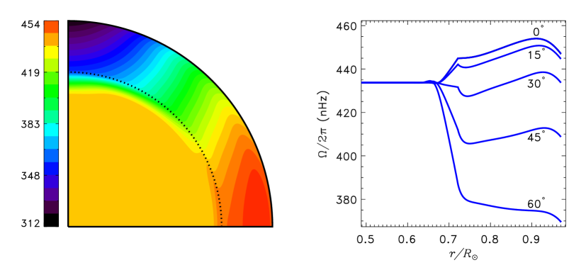
Figure 1: Angular velocity isolines (left) and depth profiles of the rotation rate for several latitudes (right) for the model of the solar differential rotation.

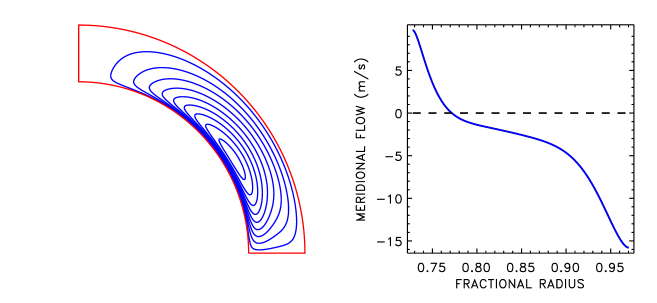
Figure 2: Stream–lines of meridional flow (left) and radial profile of meridional velocity for 45° latitude (right) for the solar model. Negative velocity means poleward flow.

The computed meridional flow is shown in Fig. 2. The direction and amplitude of the surface flow are close to observations (Komm, Howard & Harvey 1993). Note that the flow at the bottom is not small compared to the surface. This is a quite general result also found in computations for other stars. The stagnation point in Fig. 2 is close to the bottom so that the downward increase of density does not lead to a slow deep circulation. Below the convection zone, the meridional flow rapidly decreases with depth. The distance of the flow penetration into the tachocline is small compared to the tachocline thickness (Gilman & Miesch, 2004; Kitchatinov & Rüdiger, 2006).

The meridional flow is closely related to the Taylor–Proudman balance. This can be seen from the meridional flow equation

$${\cal D}(\psi)\ =\ \sin\theta\ r{\partial\Omega^{2}\over\partial z}\ -\ {g\over c_{\rm p}r}{\partial S\over\partial\theta},$$ (17)

(Kitchatinov & Rüdiger, 1999). In this equation, the left side describes the viscous drag due to the meridional flow (its relation to the eddy viscosity tensor is given by (25) and (11)), $\partial/\partial z=\cos\theta\partial/\partial r-r^{-1}\sin\theta\partial/\partial\theta$ is the spatial derivative along the rotation axis. The two terms in the right side of (17) represent the meridional flow driving by nonconservative parts of centrifugal and buoyancy forces, i.e., the centrifugal and baroclinic drivings of meridional flow, respectively. The characteristic value of each of these two terms is large compared to the left side. Accordingly, the two terms nearly balance each other in the bulk of convection zone. Consequences of the Taylor–Proudman balance for the solar rotation law have been analyzed by BRD89; Durney (1999). Deviations of isorotational surfaces from a cylindrical shape are possible due to the latitudinal inhomogeneity of entropy, which in turn can result from the anisotropy of the convective heat transport. The Taylor–Proudman balance is currently rediscussed in the context of a new hypothesis on the coincidence of the isorotational and isentropic surfaces in rotating stars (Balbus, 2009; Balbus et al., 2009).

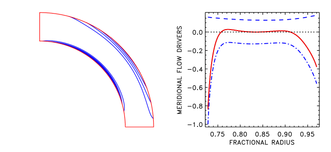
Figure 3: Right: Dependencies of the baroclinic (dashed) and centrifugal (dashed-dotted) terms of (17) and their sum (full line) on the radius for latitude 45°. The plotted values are normalized so that the maximum absolute value equals one. The dotted line shows level zero. Left: Isolines of the left side of (17). Taylor–Proudman balance is fulfilled in the bulk of the convection zone but not close to the boundaries.

Fig. 3 shows the contributions of the centrifugal and baroclinic terms in (17), and their sum for the present model of the solar rotation. The bulk of the convection zone is very close to Taylor–Proudman balance. There are, however, boundary layers where the balance is violated and the layers are not very thin (cf. Balbus et al. 2009). Similar results on the Taylor–Proudman balance are provided by 3D numerical simulations (Miesch et al. 2006; Brun, Antia, and Chitre 2010).

In (17), we see that deviations from balance produce a meridional flow. Observations of the global meridional flow on the Sun (Komm et al., 1993; Zhao & Kosovichev, 2004) indicate that certain deviations from Taylor–Proudman balance are present.

3.2 MOST–stars

The main problem with applying the differential rotation model to individual stars is to specify the (input) stellar parameters. Of the two stars – $\epsilon$ Eridani and $\kappa^{1}$ Ceti – whose differential rotation was measured using the MOST-data (Croll et al., 2006; Walker et al., 2007), $\epsilon$ Eri presents much less difficulties because all the required parameters were estimated by Soderblom & Däppen (1989).

We used the EZ code of stellar evolution by Paxton (2004) to define the structure of a main-sequence star of given mass, age, and composition and infer the input parameters for our simulations from the structure model. Hydrogen content was fixed to $X=0.7$. The parameters used to model the differential rotation of MOST-stars are given in Table 1. The parameters of $\epsilon$ Eri given by Soderblom & Däppen (1989) can be closely reproduced by the structure model of $0.8M_{\odot}$ star with metallicity $Z=0.01$ and an age of 1 Gyr. The parameters of $\kappa^{1}$ Ceti are less certain. Those used in differential rotation measurements (Rucinski et al., 2004; Walker et al., 2007) can be roughly reproduced by the structure model of a $1M_{\odot}$ star with $Z=0.02$ at the age of about 600 Myr.

Table 1: Input parameters of the differential rotation models for MOST-stars.

Star	$M/M_{\odot}$	$R/R_{\odot}$	$L/L_{\odot}$	$Z$	Age, Gyr	$P_{\mathrm{rot}}$
$\epsilon$ Eri	0.8	0.724	0.337	0.01	1	11
$\kappa^{1}$ Ceti	1.0	0.907	0.758	0.02	0.6	9

$P_{\mathrm{rot}}$ is in days.

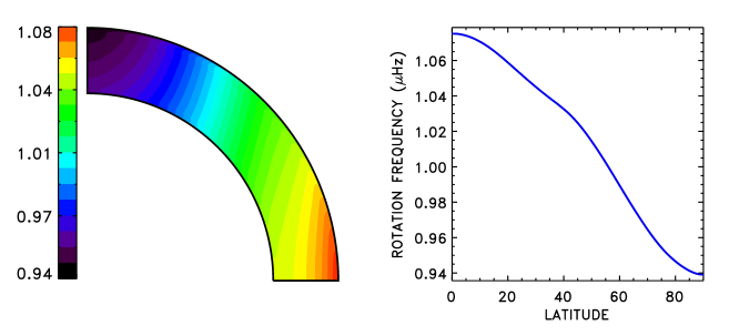
Figure 4: Angular velocity isolines (left) and surface profile of the rotation rate (right) for the differential rotation model of $\epsilon$ Eridani.

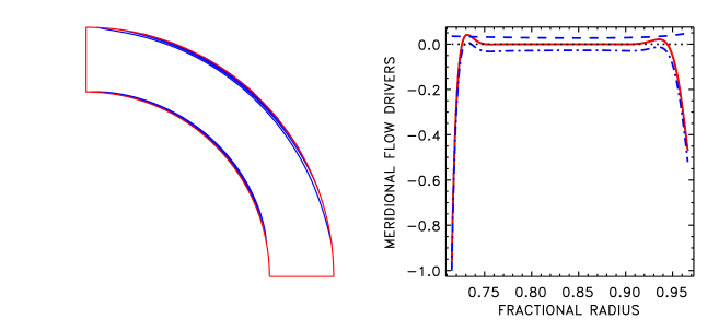
Figure 5: Same as in Fig. 3 but for the differential rotation model of $\epsilon$ Eridani.

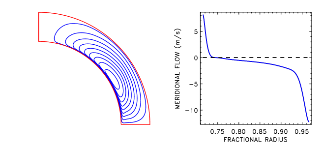
Figure 6: Simulated meridional flow of $\epsilon$ Eridani. Stream lines are shown in the left panel and the right panel shows the depth profile of the meridional velocity for latitude 45°.

Fig. 4 shows the results of differential rotation simulation for $\epsilon$ Eri. The relative magnitude of the surface differential rotation can be estimated with the parameter

$$\alpha_{{}_{\mathrm{DR}}}=1-\frac{\Omega_{\mathrm{pole}}}{\Omega_{\mathrm{eq}}}.$$ (18)

Our model gives the value of $\alpha_{{}_{\mathrm{DR}}}=0.127$ for $\epsilon$ Eri, close to the observational value of $\alpha_{{}_{\mathrm{DR}}}=0.11$ (Croll et al., 2006). The agreement for $\kappa^{1}$ Ceti is not so close: $\alpha_{{}_{\mathrm{DR}}}=0.130$ is the computational value and $\alpha_{{}_{\mathrm{DR}}}=0.09$ is the result of measurements (Walker et al., 2007). The simulated rotation laws for both ‘moderate rotators’ are quite similar. The dependence of the rotation rate on the latitude in Fig. 4 is not as smooth as for the solar model. There is a ‘peculiarity’ in the surface profile located around the latitude where the angular velocity isoline tangential to the inner boundary at the equator arrives at the surface. We always find such a peculiarity in rotation laws computed for stars rotating considerably faster than the Sun. This means that the often used approximation

$$\Omega=\Omega_{\mathrm{eq}}\left(1-\alpha_{{}_{\mathrm{DR}}}\cos^{2}\theta\right)$$ (19)

may not be very accurate. This peculiarity also means that moderate rotators are much closer to the strict Taylor–Proudman balance than the Sun. This balance is illustrated by Fig. 5. The centrifugal and baroclinic terms in the meridional flow equation (17) strictly balance each other everywhere except for the thin boundary layers. Violation of this balance in the layers excites a meridional flow. Accordingly, the meridional flow of Fig. 6 is highly concentrated at the boundaries. The bottom flow is not small compared to the top but the flow in the bulk of the convection zone away from the boundary layers is slow. We shall see that the boundary layers are even more pronounced in rapid rotators.

There is an increasing belief that meridional flow is important for solar (Choudhuri, Schüssler & Dikpati, 1995) and stellar (Jouve, Brown & Brun, 2010) dynamos. The flow structure prescribed in advection-dominated dynamo models is, however, different from the flow predicted by stellar circulation models.

3.3 Rapid rotators

Simulations of differential rotation were performed for two young stars – AB Doradus and LQ Hydrae – that seem to be the most frequent observational targets among the rapid rotators. Other dwarf stars for which the differential rotation was measured by Doppler imaging are either not yet settled on the main sequence or their structure parameters are difficult to determine. The parameters used in differential rotation simulations that also help to reproduce closely the observational structure parameters of AB Dor (Donati & Collier Cameron, 1997; Ortega et al., 2007; Guirado Marti-Vidal & Marcaide, 2008) and LQ Hya (Kővári et al., 2004) are listed in Table 2.

Table 2: Input parameters of the differential rotation models for AB Doradus and LQ Hydrae.

Star	$M/M_{\odot}$	$R/R_{\odot}$	$L/L_{\odot}$	$Z$	Age	$P_{\mathrm{rot}}$
AB Dor	0.9	0.803	0.438	0.02	70	0.514
LQ Hya	0.77	0.698	0.273	0.01	100	1.6

Age is given in Myr, $P_{\mathrm{rot}}$ – in days.

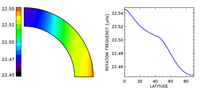
Figure 7: Angular velocity isolines (left) and latitude dependence of the surface rotation frequency (right) for the differential rotation model of AB Dor.

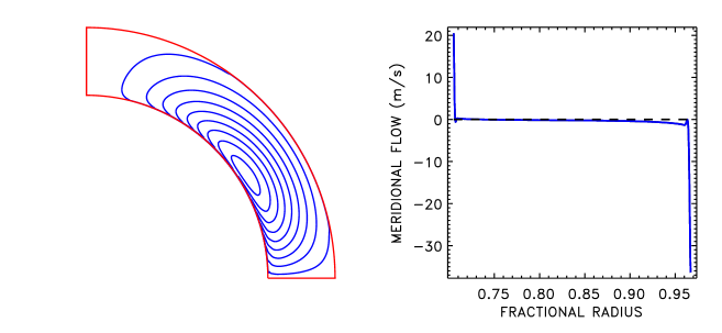
Figure 8: Simulated meridional flow of AB Dor. The left panel shows the stream lines and the right panel presents the depth profile of meridional velocity for the latitude of 45^∘. Negative velocity means poleward flow.

Figs. 7 and 8 show the modelled differential rotation and meridional flow of AB Dor. The computed differential rotation measure $\alpha_{{}_{\mathrm{DR}}}=4.37\times 10^{-3}$ is very close to the observational value of $4.5\times 10^{-3}$ (Donati & Collier Cameron, 1997). The peculiarity in the surface profile of rotation rate discussed in Section 3.2 is even more pronounced in Fig. 7 compared to the moderate rotation case of Fig. 4. The profile can be only roughly approximated by the $\cos^{2}\theta$-law of (19). If the approximation is nevertheless used to describe the rotation of the stellar spots, it may lead to a seeming variation of the differential rotation with time. The spots positioned at different latitudes for different observational epochs would lead to different $\alpha_{{}_{\mathrm{DR}}}$ suggesting torsional oscillations even for a steady rotation law.

Observational estimates of the differential rotation of the slower rotating LQ Hya have a wide spread (Barnes et al., 2005). We can only state that the differential rotation measure of our model, $\alpha_{{}_{\mathrm{DR}}}=1.28\times 10^{-2}$, is within the range of observational estimates.

The meridional flow of Fig. 8 shows an extreme concentration in the boundary layers. The flow consists of two near-boundary jets linked by a very slow circulation in the bulk of the convection zone. Such a boundary-layer flow is, probably, not important for dynamos. However, the distributed (solar-type) flow of Fig. 2 may be significant for magnetic field transport. The meridional circulation changes from a distributed flow (Fig. 2) to the near-boundary jets (Fig. 8) with an increasing rotation rate. This change of meridional flow may cause a change in the dynamo regime that may be the reason for the two separate branches for fast and slow rotators in the dependence of the dynamo-cycle period on the stellar rotation rate found by Saar & Brandenburg (1999).

3.4 Temperature dependence

Fig. 9 shows the dependence of the surface differential rotation on stellar mass computed with our model. The computations were made for young stars just arrived on the main sequence and rotating with a period of 1 day. Models were produced for the mass range from $0.4M_{\odot}$ to $1.2M_{\odot}$ (with $0.05M_{\odot}$ spacing). These computations cover the surface temperature range from about 3600 K to 6500 K or spectral types from K2 to F6 which roughly corresponds to the range for which Barnes et al. (2005) constructed the temperature dependence of the surface differential rotation detected by Doppler imaging. The computations were made for three metallicity values of $Z=0.01,\ 0.02,\ 0.03$. For a given stellar mass, the results depend on the chemical composition, so that for a mass of $1.2M_{\odot}$, the surface differential rotation differs by a factor of about 10 between the cases of $Z=0.01$ and $Z=0.03$.

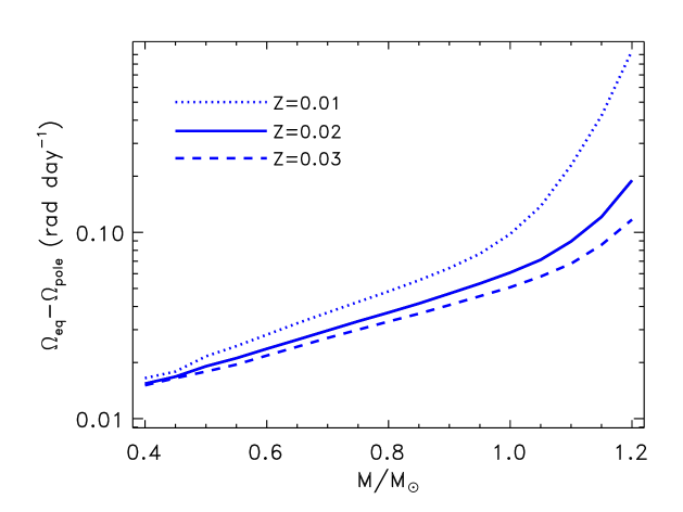
Figure 9: Surface differential rotation of ZAMS-stars with $P_{\mathrm{rot}}=1$ day as a function of stellar mass. Three lines show the results of computations for metallicities $Z=0.01$ (dotted), $Z=0.02$ (full line), and $Z=0.03$ (dashed).

The metallicity dependence almost disappear, however, when the differential rotation is plotted as a function of surface temperature (Fig. 10). So, the effective temperature is indeed convenient for parameterizing the differential rotation of young stars (Barnes et al., 2005). An even better scaling can be found by using the Coriolis number of (4). The results for different chemical compositions practically coincide on the plot of differential rotation as a function of the Coriolis number. As the Coriolis number is not directly observable, we shall keep using the surface temperature.

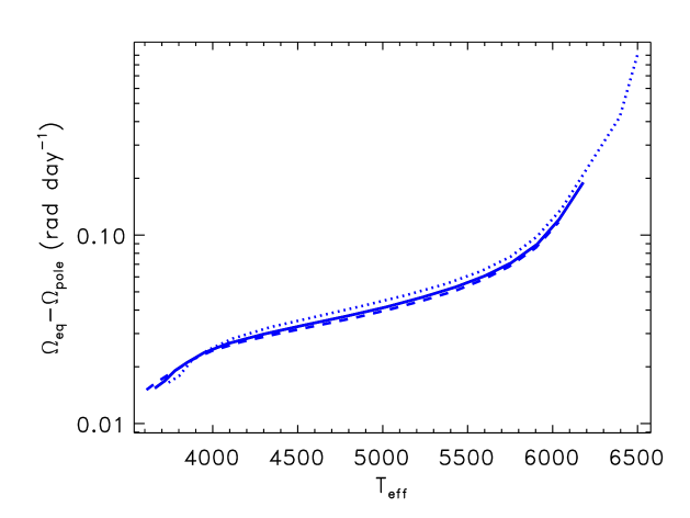
Figure 10: Same differential rotation as in Fig. 9 but shown as a function of surface temperature. The results for different metallicities of $Z=0.01$ (dotted line), $Z=0.02$ (full line), and $Z=0.03$ (dashed line) now differ by little.

Figs. 9 and 10 predict that relatively hot convective stars can possess strong differential rotations with pole-equator lap times shorter than 10 days. This is larger than the strongest differential rotation observed to date (Jeffers & Donati, 2008). The question arises whether a strong differential rotation implies over-normal dynamo-activity. The results of Fig. 11 suggest a negative answer. The figure shows the $C_{\Omega}$ dynamo-number of (1) as a function of surface temperature.

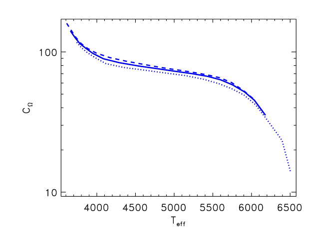
Figure 11: $C_{\Omega}$ dynamo-number of (1) as a function of surface temperature. The lines of different styles show the results for different metallicities, $Z=0.01$ (dotted), $Z=0.02$ (full line), and $Z=0.03$ (dashed).

The $C_{\Omega}$-parameter was computed for the middle of the convection zone using the isotropic part of the eddy magnetic diffusivity $\eta_{{}_{\mathrm{T}}}=\chi_{{}_{\mathrm{T}}}\phi(\Omega^{*})$ (that coincides with the eddy conductivity; Kitchatinov et al. 1994) and latitudinal differential rotation (the radial inhomogeneity of rotation is relatively small). The estimation assumes that dynamos of young stars are distributed over their convection zones (Donati, 1999).

The $C_{\Omega}$ of Fig. 11 declines sharply with temperature for F-stars indicating that the strong differential rotation of these stars is not efficient at producing toroidal magnetic fields. This is in agreement with the idea of Durney & Latour (1978) that convective dynamos cease to operate at about spectral type F6. The $C_{\Omega}$ increases steadily with decreasing temperature. This is because the convection slows down in low mass stars to decrease eddy diffusion. The decline of magnetic eddy diffusivity overpowers the decrease of differential rotation to produce a larger $C_{\Omega}$ in smaller stars. The largest $C_{\Omega}$ belong to M-dwarfs. This is in contrast to the common belief that the small differential rotation of M-stars cannot be important for dynamos and that the magnetic fields of these stars are generated by the $\alpha^{2}$-mechanism. The $\alpha^{2}$ dynamos produce nonaxisymmetric global fields. However, observations favour an axial symmetry of the global magnetic structure of M-stars (Donati et al., 2006). This may be explained by the effect of differential rotation, which is small in low-mass stars, but efficient in winding magnetic fields.

The gravitational darkening of (14) is not significant for our results. Neglecting the darkening effect reduces the computed differential rotation normally by less than 1 per cent (by several per cent in extreme cases of rapidly rotating F-stars).

4 Summary

This paper presents the first results of the new mean-field model of stellar differential rotation, which improves on its former formulation (Kitchatinov & Rüdiger, 1999), to cover the case of rapidly rotating stars with $P_{\mathrm{rot}}\sim 1$ day.

The model reproduces very closely helioseismological inversions for the internal solar rotation. The simulated meridional flow at the bottom of the solar convection zone has an amplitude of about 10 m s^-1 that is not small compared to the surface flow. The near-bottom equator-ward flow can be important for the solar dynamo.

The meridional flow in stars rotating faster than the Sun is increasingly concentrated in boundary layers near the top and bottom of the convection zone as the rotation rate increases. We interpret this boundary-layer structure of the meridional flow as an effect of thin boundary layers where Taylor–Proudman balance is violated. The change of the meridional flow from distributed to boundary-layer structure may be the reason for the change of dynamo regime between slow and fast rotators (Saar & Brandenburg, 1999).

The differential rotation model was applied to four individual stars including two moderate ($P_{\mathrm{rot}}\sim 10$ days) and two fast ($P_{\mathrm{rot}}\sim 1$ day) rotators. In two cases, for which the structure parameters of the stars are well known, close agreement with observations was found. In all cases, the computed rotation laws were not so close to the $\sin^{2}(\mathrm{latitude})$-profile of equation (19) as it is for the Sun.

The computations for the rapidly rotating ($P_{\mathrm{rot}}=1$ day) ZAMS-stars show that the surface temperature, $T_{\mathrm{eff}}$, is a convenient parameter for the differential rotation: when considered as a function of $T_{\mathrm{eff}}$, the differential rotation loses its dependence on the chemical composition of a star that otherwise can be quite pronounced. The differential rotation increases with $T_{\mathrm{eff}}$ and the rotation rate difference between equator and poles can reach almost 1 rad day^-1 for the hottest F-stars we considered.

This strong differential rotation is, however, not efficient for dynamos. The standard $C_{\Omega}$-parameter of the dynamo models of equation (1) that measures the efficiency of toroidal field production by differential rotation decreases with $T_{\mathrm{eff}}$. Contrary to intuitive expectation, the small differential rotation of M-stars is important for magnetic field generation. This may be the reason for the closeness of the observed magnetic structure of M-stars to axial symmetry (Donati et al., 2006).

As a perspective for future work, theoretical construction of the dependence of differential rotation on stellar age and temperature based on girochronology (Barnes, 2008) can be pointed out.

Appendix A Motion equations

A.1 Reynolds stress

The Reynolds stress tensor is related to the fluctuating velocity correlation of (10) and (11), $R_{ij}=-\rho Q_{ij}$. The part $Q^{\Lambda}_{ij}$ of the correlation tensor, which represents the $\Lambda$-effect of the non-viscous transport of angular momentum in stratified rotating fluids, reads

$$Q^{\Lambda}_{ij} = \nu_{{}_{\mathrm{T}}}\left(\frac{\alpha_{{}_{\mathrm{MLT}}}}{\gamma}\right)^{2}\bigg{(}\left(J_{0}(\Omega^{*})+aI_{0}(\Omega^{*})\right)\times$$ (20)

$$\left(\hat{r}_{i}\varepsilon_{jkl}+\hat{r}_{j}\varepsilon_{ikl}\right)-\left(J_{1}(\Omega^{*})+aI_{1}(\Omega^{*})\right)\times$$

$$\frac{\left(\hat{\mbox{\boldmath$r$}}\cdot{\mbox{\boldmath$\Omega$}}\right)}{\Omega^{2}}\left(\Omega_{i}\varepsilon_{jkl}+\Omega_{j}\varepsilon_{ikl}\right)\bigg{)}\Omega_{k}\hat{r}_{l},$$

where $\hat{\mbox{\boldmath$r$}}$ is the radial unit vector, $a$ is a parameter of convection anisotropy ($a=2$ in all our computations), and $\gamma=c_{\mathrm{p}}/c_{\mathrm{v}}$. Recent discussions of the $\Lambda$-effect can be found in Rüdiger & Kitchatinov (2007a) and Garaud et al. (2010). The origin of the expression (20) for the $\Lambda$-effect was discussed by Kitchatinov & Rüdiger (2005) where expressions for the functions $J_{0},\ J_{1},\ I_{0},\ I_{1}$ of the Coriolis number $\Omega^{*}$ are also given.

The viscous part of the Reynolds stress is controlled by the viscosity tensor of (11). The viscosity is anisotropic due to the rotational influence on turbulent convection,

$${\cal N}_{ijkl} = \nu_{{}_{\mathrm{T}}}\big{(}\phi_{1}(\Omega^{*})\left(\delta_{ik}\delta_{jl}\ +\ \delta_{jk}\delta_{il}\right)$$ (21)

$$+ \phi_{2}(\Omega^{*})\big{(}\delta_{il}\hat{\Omega}_{j}\hat{\Omega}_{k}+\delta_{jl}\hat{\Omega}_{i}\hat{\Omega}_{k}$$

$$+ \delta_{ik}\hat{\Omega}_{j}\hat{\Omega}_{l}+\delta_{jk}\hat{\Omega}_{i}\hat{\Omega}_{l}+\delta_{kl}\hat{\Omega}_{i}\hat{\Omega}_{j}\big{)}$$

$$+ \phi_{3}(\Omega^{*})\ \delta_{ij}\delta_{kl}\ -\ \phi_{4}(\Omega^{*})\ \delta_{ij}\hat{\Omega}_{k}\hat{\Omega}_{l}$$

$$+ \phi_{5}(\Omega^{*})\ \hat{\Omega}_{i}\hat{\Omega}_{j}\hat{\Omega}_{k}\hat{\Omega}_{l}\big{)}.$$

The viscosity quenching functions, $\phi_{n}(\Omega^{*}),\ n=1,...,5$, can be found in Kitchatinov et al. (1994). The eddy viscosity $\nu_{{}_{\mathrm{T}}}$ for a non-rotating fluid is expressed in terms of the entropy gradient

$$\nu_{{}_{\mathrm{T}}}=-\frac{\tau\ell^{2}g}{15c_{\mathrm{p}}}\frac{\partial S}{\partial r}.$$ (22)

A.2 Angular velocity equation

The azimuthal component of (8) gives the continuity equation for the angular momentum flux,

$$\frac{1}{r^{2}\rho}\frac{\partial}{\partial r}\left(\rho r^{3}Q_{r\phi}\right)+\frac{1}{\sin^{2}\theta}\frac{\partial}{\partial\theta}\left(\sin^{2}\theta\ Q_{\theta\phi}\right) +$$

$$\frac{1}{r^{2}\rho}\frac{\partial(r^{2}\Omega)}{\partial r}\frac{\partial\psi}{\partial\theta}-\frac{1}{\rho\sin^{2}\theta}\frac{\partial(\sin^{2}\theta\ \Omega)}{\partial\theta}\frac{\partial\psi}{\partial r} = 0,$$ (23)

where the first and the second lines describe angular momentum transport by convection and meridional flow respectively. On using (11) and (20) – (22), the convective fluxes of angular momentum can be written as follows

$$Q_{\theta\varphi} = \sin\theta\ {\tau\ell^{2}g\over 15c_{\mathrm{p}}}{\partial S\over\partial r}\bigg{\{}\phi_{1}(\Omega^{*}){\partial\Omega\over\partial\theta}$$

$$- \phi_{2}(\Omega^{*})\sin\theta\left(\cos\theta\ r{\partial\Omega\over\partial r}\ -\ \sin\theta{\partial\Omega\over\partial\theta}\right)$$

$$- \Omega\left({\alpha_{\rm MLT}\over\gamma}\right)^{2}\sin\theta\cos\theta\ \left(J_{1}(\Omega^{*})+aI_{1}(\Omega^{*})\right)\bigg{\}},$$

$$Q_{r\varphi} = \sin\theta\ {\tau\ell^{2}g\over 15c_{\mathrm{p}}}{\partial S\over\partial r}\bigg{\{}\phi_{1}(\Omega^{*})r{\partial\Omega\over\partial r}$$ (24)

$$+ \phi_{2}(\Omega^{*})\cos\theta\left(\cos\theta\ r{\partial\Omega\over\partial r}\ -\ \sin\theta{\partial\Omega\over\partial\theta}\right)$$

$$- \Omega\left({\alpha_{{}_{\mathrm{MLT}}}\over\gamma}\right)^{2}\big{(}J_{0}(\Omega^{*})+aI_{0}(\Omega^{*})$$

$$- \cos^{2}\theta\ \left(J_{1}(\Omega^{*})+aI_{1}(\Omega^{*})\right)\big{)}\bigg{\}}.$$

With the angular momentum fluxes (24), (23) governs the angular velocity distribution in the convection zone.

A.3 Meridional flow equation

The equation (17) for the meridional flow can be found as the azimuthal component of the curled equation (8). The left part,

$${\cal D}(\psi)=\varepsilon_{\phi jk}\frac{\partial}{\partial r_{j}}\left(\frac{1}{\rho}\frac{\partial\left(\rho Q^{\nu}_{kl}\right)}{\partial r_{l}}\right),$$ (25)

of this equation describes the viscous drag to the meridional flow. In spherical coordinates, (25) reads

$${\cal D}(\psi) = \frac{1}{r}\frac{\partial}{\partial r}\left(\frac{1}{\rho r^{2}}\frac{\partial(\rho r^{3}Q^{\nu}_{r\theta})}{\partial r}\right)$$ (26)

$$- \frac{1}{r^{2}}\frac{\partial}{\partial\theta}\left(\frac{1}{\sin\theta}\frac{\partial\left(\sin\theta\ Q^{\nu}_{r\theta}\right)}{\partial\theta}\right)$$

$$- \frac{1}{r\rho}\frac{\partial\rho}{\partial r}\frac{\partial Q^{\nu}_{rr}}{\partial\theta}+\frac{1}{r}\frac{\partial^{2}}{\partial r\partial\theta}\left(Q^{\nu}_{\theta\theta}-Q^{\nu}_{rr}\right)$$

$$+ \frac{\cos\theta}{r\sin\theta}\frac{\partial}{\partial r}\left(Q^{\nu}_{\theta\theta}-Q^{\nu}_{\phi\phi}\right)$$

$$+ \frac{1}{r^{2}}\frac{\partial}{\partial\theta}\left(Q^{\nu}_{\theta\theta}+Q^{\nu}_{\phi\phi}-2Q^{\nu}_{rr}\right).$$

The explicit expression for ${\cal D}(\psi)$ in terms of the stream function is very complicated and never used in practice. Instead, $Q^{\nu}_{r\theta}$, $u_{\theta}$ and a certain combination of diagonal components of $Q^{\nu}_{ij}$ are introduced as new dependent variables when solving the meridional flow equation. The expressions for these new variables in terms of the stream function can by found from (11), (12), and (21).

References

- Balbus (2009) Balbus S.A., 2009, MNRAS, 395, 2056
- Balbus et al. (2009) Balbus S.A., Bonart J., Latter H.N., Weiss N.O., 2009, MNRAS, 400, 176
- Barnes (2008) Barnes S.A., 2008, IAUS, 258, 345
- Barnes et al. (2005) Barnes J.R., Collier Cameron A., Donati J.-F., James D.J., Marsden S.C., Petit P., 2005, MNRAS, 357, L1
- Brun & Rempel (2009) Brun A.S., Rempel M., 2009, SSRv, 144, 151
- Brun, Antia & Chitre (2010) Brun A.S., Antia H.M., Chitre S.M., 2010, A&A, 510, 33
- Choudhuri, Schüssler & Dikpati (1995) Choudhuri A.R., Schüssler M., Dikpati M., 1995, A&A, 303, L29
- Christensen-Dalsgaard (2008) Christensen-Dalsgaard J., 2008, IAUS, 252, 135
- Collier Cameron & Donati (2002) Collier Cameron A., Donati J.-F., 2002, MNRAS, 329, L23
- Croll et al. (2006) Croll B., Walker G.A.H., Kuschnig R. et al., 2006, ApJ, 648, 607
- Donati (1996) Donati J.-F., 1996, IAUS, 176, 53
- Donati (1999) Donati J.-F., 1999, MNRAS, 302, 457
- Donati & Collier Cameron (1997) Donati J.-F., Collier Cameron A., 1997, MNRAS, 291, 1 1996, IAUS, 176, 53
- Donati, Collier Cameron & Petit (2003) Donati J.-F., Collier Cameron A., Petit P., 2003, MNRAS, 345, 1187
- Donati et al. (2006) Donati J.-F., Forveille T., Collier Cameron A., Barnes J.R., Delfosse X., Jardine M.M., Valenti J.A., 2006, Sci, 311, 633
- Durney (1989) Durney B.R., 1989, ApJ, 338, 509
- Durney (1999) Durney B.R., 1999, ApJ, 511, 945
- Durney & Latour (1978) Durney B.R., Latour J., 1978, GApFD, 9, 241
- Garaud et al. (2010) Garaud P., Ogilvie G.I., Miller N., Stellmach S., 2010, arXiv:astro-ph/1004.3239
- Gilman & Miesch (2004) Gilman P.A., Miesch M.S., 2004, ApJ, 611, 568
- Guirado Marti-Vidal & Marcaide (2008) Guirado J.C., Marti-Vidal I., Marcaide J.M., 2008, IAUS, 248, 496
- Jeffers & Donati (2008) Jeffers S.V., Donati J.-F., 2008, MNRAS, 390, 635
- Jouve, Brown & Brun (2010) Jouve L., Brown B.P., Brun A.S., 2010, A&A, 509, 32