Cosmological rotating black holes in five-dimensional fake supergravity

Abstract

In recent series of papers, we found an arbitrary dimensional, time-evolving and spatially-inhomogeneous solutions in Einstein-Maxwell-dilaton gravity with particular couplings. Similar to the supersymmetric case the solution can be arbitrarily superposed in spite of non-trivial time-dependence, since the metric is specified by a set of harmonic functions. When each harmonic has a single point source at the center, the solution describes a spherically symmetric black hole with regular Killing horizons and the spacetime approaches asymptotically to the Friedmann-Lemaître-Robertson-Walker (FLRW) cosmology. We discuss in this paper that in 5-dimensions this equilibrium condition traces back to the 1st-order “Killing spinor” equation in “fake supergravity” coupled to arbitrary ${\rm U}(1)$ gauge fields and scalars. We present a 5-dimensional, asymptotically FLRW, rotating black-hole solution admitting a nontrivial “Killing spinor,” which is a spinning generalization of our previous solution. We argue that the solution admits nondegenerate and rotating Killing horizons in contrast with the supersymmetric solutions. It is shown that the present pseudo-supersymmetric solution admits closed timelike curves around the central singularities. When only one harmonic is time-dependent, the solution oxidizes to 11-dimensions and realizes the dynamically intersecting M2/M2/M2-branes in a rotating Kasner universe. The Kaluza-Klein type black holes are also discussed.

I Introduction

Supersymmetric solutions in supergravity have played an important rôle in the development of string theory and the anti-de Sitter(AdS)/conformal field theory (CFT)-correspondence. A pioneer work in this direction was the great success of microscopic deviation of black hole entropy from the viewpoint of intersecting D-branes. By virtue of the saturation of Bogomol’nyi-Prasad-Sommerfield (BPS) bound, the supersymmetric solutions can provide arena for exploring the non-perturbative limits of string theory. The BPS equality constraints the supersymmetry variation spinor to satisfy the 1st-order differential equation. Such a covariantly constant spinor is called a Killing spinor, which ensures that the energy is positively bounded by central charges, guaranteeing the stability of the theory. The relationship between vacuum stability and BPS states was suggested by Witten’s positive energy theorem Witten:1981mf , and later validated firmly by GH1982 ; PET .

From a standpoint of pure gravitating object, black hole solutions admitting a Killing spinor are sharply distinguished from non-BPS black hole solutions. These BPS configurations are dynamically very simple. First of all, BPS black hole solutions necessarily have zero Hawking temperature (the converse is not true), implying that the horizon is degenerate. Accordingly they are free from thermal excitation. Such a non-bifurcating horizon universally admits a throat infinity and enhanced isometries of ${\rm SO}(2,1)$ Kunduri:2007vf . Secondly, most BPS solutions satisfy “no-force” condition. For example, we are able to superpose the extreme Reissner-Nordström solutions at our disposal due to the delicate compensation between the gravitational attractive force and the electromagnetic repulsive force. The resulting multicenter metric, originally found by Majumdar and Papapetrou, maintains static equilibrium and describes collection of charged black holes Hartle:1972ya . This property can be ascribed to the complete linearization of field equations. Besides these, all the BPS black holes are known to be strictly stationary, viz, the ergoregion does not exist even if the black hole has nonvanishing angular momentum. Dynamically evolving states are not compatible with supersymmetry.

Then, to what extent these known intuitive properties continue to hold? Motivated by this inquiry it is important to explore general properties and classify BPS solutions. A first progress was made by Tod, who catalogued all the BPS solutions admitting nontrivial Killing spinors of 4-dimensional $\mbox{$\mathcal{N}$}=2$ supergravity Tod , inspired by the early study of Gibbons and Hull GH1982 . Recently, Gauntlett et al. GGHPR were able to obtain general supersymmetric solutions in 5-dimensional minimal supergravity exploiting bilinears constructed from a Killing spinor. Since their technique has no restriction upon the spacetime dimensionality, reference GGHPR has sparked a considerable development in the classifications of supersymmetric solutions in various supergravities Gauntlett:2003fk ; Gutowski:2003rg ; Caldarelli:2003pb ; GR . This formalism is useful for finding supersymmetric black holes Gutowski:2004ez ; Kunduri:2006ek and black rings Elvang:2004rt ; Elvang:2004ds ; Gauntlett:2004qy , and for proving uniqueness theorem of certain black holes Reall2002 ; Gutowski:2004bj . It turns out that all the BPS black holes fulfill above mentioned properties except for the equilibrium condition which is valid only in the ungauged case.

On the other hand, non-BPS black hole solutions–especially the time-dependent black hole solutions–have been much less understood. In this paper we address some properties of cosmological black-hole solutions which have an interpretation as arising from the gauged supergravity with non-compact R-symmetry gauged. The most simplest theory is the 4-dimensional minimal de Sitter supergravity consisting of the graviton, the Maxwell fields and a positive cosmological constant Pilch:1984aw . A time-dependent solution in this theory was found by Kastor and Traschen KT ; London , which is the generalization of Majumdar-Papapetrou solution in the de Sitter background. The Kastor-Traschen solution describes coalescing black holes in the contracting de Sitter universe (or splitting white holes in the expanding de Sitter universe) and inherits some salient characteristics from the Majumdar-Papapetrou solution. The reason why multicenter metric is in mechanical equilibrium irrespective of the time-dependence is attributed to the first-order “BPS equation” that extremizes the action, allowing the complete linearization of field equations. Since these “BPS” states are not truly supersymmetric in the usual sense, they are referred to as pseudo-supersymmetric and the corresponding theory is called a “fake” supergravity. Recently, all pseudo-supersymmetric solutions in 4- and 5-dimensional fake de Sitter fake supergravity were classified using the spinorial geometry method Gutowski:2009vb ; Grover:2008jr (see Meessen:2009ma for a non-Abelian generalization).

In this paper, we discuss properties of pseudo-supersymmetric solutions of 5-dimensional fake supergravity with arbitrary number of ${\rm U}(1)$ gauge fields and scalar fields. Some time-dependent black hole solutions in this theory have been available so far Behrndt:2003cx ; Klemm:2000gh , but their properties and causal structures are yet to be explored. Even for the simplest case in which the harmonic function is sourced by a single point mass, the spacetime is highly dynamical except in the de Sitter supergravity. In the present case the background spacetime is the Friedmann-Lemaître-Robertson-Walker (FLRW) cosmology. (In the context of fake supergravity, it is argued that the FLRW cosmologies are duals of supersymmetric domain walls. See DW_FRW for details.) A series of recent papers of present authors MN ; MNII revealed that the solution of a single point source found in MOU ; GMII actually describes a charged black hole in the FLRW cosmology. Though the metric in MOU ; GMII were shown to be the exact solutions of Einstein-Maxwell-dilaton system, we show in this paper that the 5-dimensional solutions of MOU ; MNII in fact satisfy the 1st-order BPS equation in fake supergravity. The pseudo-supersymmetry is indeed consistent with an expanding universe. This work will establish new insights for black holes in time-dependent and non-supersymmetric backgrounds.

The main concern in this paper is to see the effects of black-hole rotation in 5-dimensions by restricting to the single point mass case. As it turns out, rotation makes the properties of spacetime much richer. Our work is organized as follows. In the next section we describe a fake supergravity model and derive (in a gauge different from Klemm:2000vn ) a rotating, time-dependent solution preserving the pseudo-supersymmetry. Section III is devoted to explore physical and geometrical properties of the spacetime. We establish that the black hole horizon is generated by a rotating Killing horizon, in sharp contrast with the supersymmetric black-hole horizon which admits a non-rotating degenerate Killing horizon without an ergoregion. It is also demonstrated that the solution generally admits closed timelike curves in the vicinity of timelike singularities (with trivial fundamental group). Combining the analysis of the near-horizon geometries, we shall elucidate the causal structures by illustrating Carter-Penrose diagrams. In section IV the liftup and reduction scheme of the 5-dimensional solution is accounted for. It is shown that the 5-dimensional solutions derived in MOU ; MNII and in section III are elevated to describe the non-BPS dynamically intersecting M2/M2/M2-branes in 11-dimensional supergravity. Upon dimensional reduction the 4-dimensional black hole MOU ; GM is obtainable. We shall also present some Kaluza-Klein black holes in the FLRW universe. Section V gives final remarks.

We will work in mostly plus metric signature and the standard curvature conventions $2\nabla_{[\rho}\nabla_{\sigma]}V^{\mu}={R^{\mu}}_{\nu\rho\sigma}V^{\nu}$. Gamma matrix conventions are such that $\gamma_{\mu\nu\rho\sigma\tau}=i\epsilon_{\mu\nu\rho\sigma\tau}$ with $\epsilon_{01234}=1$ and $\bar{\psi}:=i\psi^{\dagger}\gamma^{0}$.

II Five dimensional solutions in minimal supergravity

The metrics obtained in MOU ; GMII ; MN ; MNII are the exact solutions of Einstein’s equations sourced by two-${\rm U}(1)$ fields and a scalar field coupled to the gauge fields. Since the solution involves two kinds of harmonic functions, it manifests mechanical equilibrium regardless of time-evolving spacetime. When each harmonic has a point source at the center, the solution in MOU ; GMII ; MN ; MNII describes a spherically symmetric black hole embedded in the FLRW cosmology. In this section, we consider a five-dimensional supergravity-type Lagrangian and present more general (pseudo) BPS solutions, which encompass the 5-dimensional solution in MOU ; MNII as special limiting cases.

Let us start from the minimal 5-dimensional gauged supergravity coupled to $N$ abelian vector multiplets. The bosonic action involves graviton, ${\rm U}(1)$ gauge fields $A^{(I)}$ ($I=1,...,N$) with real scalars $\phi^{A}$ ($A=1,...,N-1$) Gunaydin:1984ak ,

$$S= \frac{1}{2\kappa_{5}^{2}}\int\left[\left({}^{5}R+2\mathfrak{g}^{2}V\right)\star_{5}1-\mbox{$\mathcal{G}$}_{AB}{\rm d}\phi^{A}\wedge\star_{5}{\rm d}\phi^{B}\right.$$

$$\left.-G_{IJ}F^{(I)}\wedge\star_{5}F^{(J)}-\frac{1}{6}C_{IJK}A^{(I)}\wedge F^{(J)}\wedge F^{(K)}\right]\,,$$ (1)

where $F^{(I)}={\rm d}A^{(I)}$ are the field strengths of gauge fields and $\mathfrak{g}$ is the coupling constants corresponding to the reciprocal of the AdS curvature radius. $C_{IJK}$ are constants symmetric in $(IJK)$ and obey the “adjoint identity”

$$C_{IJK}C_{J^{\prime}(LM}C_{PQ)K^{\prime}}\delta^{JJ^{\prime}}\delta^{KK^{\prime}}=\frac{4}{3}\delta_{I(L}C_{MPQ)}\,,$$ (2)

where the round brackets denote symmetrization of the suffixes. The potential $V$ can be expressed in terms of a superpotential $W$ as

$$V=6W^{2}-\frac{9}{2}\mbox{$\mathcal{G}$}^{AB}(\partial_{A}W)(\partial_{B}W)\,,$$ (3)

where $\partial_{A}X^{I}:={\rm d}X^{I}(\phi)/{\rm d}\phi^{A}$. The superpotential takes the form,

$$W=V_{I}X^{I}\,,$$ (4)

where $V_{I}$ are constants arising from an Abelian gaugings of the ${\rm SU}(2)$-R symmetry with the gauge field $A=V_{I}A^{I}$ Gunaydin:1984ak . The $N$-scalars $X^{I}$ are constrained by

$$\mbox{$\mathcal{V}$}:=\frac{1}{6}C_{IJK}X^{I}X^{J}X^{K}=1\,.$$ (5)

It is convenient to define

$$X_{I}=\frac{1}{6}C_{IJK}X^{J}X^{K}\,,$$ (6)

in terms of which Eq. (5) is simply $X_{I}X^{I}=1$. The coupling matrix $G_{IJ}$ is the metric of the “very special geometry” deWit:1992cr defined by

$$G_{IJ}:=-\frac{1}{2}\left.\frac{\partial^{2}}{\partial X^{I}\partial X^{J}}\ln\mbox{$\mathcal{V}$}\right|_{\mathcal{V}=1}=\frac{9}{2}X_{I}X_{J}-\frac{1}{2}C_{IJK}X^{K}\,,$$ (7)

with its inverse

$$G^{IJ}=2X^{I}X^{J}-6C^{IJK}X_{K}\,,$$ (8)

where $C^{IJK}=\delta^{IL}\delta^{JP}\delta^{KQ}C_{LPQ}$. The other coupling matrix $\mbox{$\mathcal{G}$}_{AB}$ is given by

$$\mbox{$\mathcal{G}$}_{AB}=G_{IJ}\partial_{A}X^{I}\partial_{B}X^{J}\,,$$ (9)

It follows that

$$X^{I}=\frac{9}{2}C^{IJK}X_{J}X_{K}\,,$$ (10)

and

$$X_{I}=\frac{2}{3}G_{IJ}X^{J}\,,\qquad X^{I}=\frac{3}{2}G^{IJ}X_{J}\,.$$ (11)

From these relations, we obtain useful expressions

$${\rm d}X_{I}=-\frac{2}{3}G_{IJ}{\rm d}X^{J}\,,\qquad{\rm d}X^{I}=-\frac{3}{2}G^{IJ}{\rm d}X_{J}\,,$$

$$X^{I}{\rm d}X_{I}=X_{I}{\rm d}X^{I}=0\,,$$

$$\mbox{$\mathcal{G}$}^{AB}\partial_{A}X^{I}\partial_{B}X^{J}=G^{IJ}-\frac{2}{3}X^{I}X^{J}.$$ (12)

Using these formulae, the potential reads

$$V=27C^{IJK}V_{I}V_{J}X_{K}\,.$$ (13)

If this theory is derived via gauging the supergravity derived from the Calabi-Yau compactification of M-Theory, $\mathcal{V}$ is the intersection form, $X^{I}$ and $X_{I}$ correspond respectively to the size of the two- and four-cycles. The constants $C_{IJK}$ are the intersection numbers of the Calabi-Yau threefold and $N$ denotes the Hodge number $h_{1,1}$ Papadopoulos:1995da .

The governing equations are the Einstein equations (varying $g^{\mu\nu}$),

$${}^{5}R_{\mu\nu}-\frac{1}{2}\left({}^{5}R+2\mathfrak{g}^{2}V\right)g_{\mu\nu}=G_{IJ}\left[(\nabla_{\mu}X^{I})(\nabla_{\nu}X^{J})-\frac{1}{2}(\nabla^{\rho}X^{I})(\nabla_{\rho}X^{J})g_{\mu\nu}+F^{(I)\rho}_{\mu}F^{(J)}_{\nu\rho}-\frac{1}{4}F^{(I)}_{\rho\sigma}F^{(J)\rho\sigma}g_{\mu\nu}\right]\,,$$ (14)

the electromagnetic field equations (varying $A^{(I)}$),

$$\nabla_{\nu}\left(G_{IJ}F^{(J)\mu\nu}\right)-\frac{1}{16}C_{IJK}\epsilon^{\mu\nu\rho\sigma\tau}F^{(J)}_{\nu\rho}F^{(K)}_{\sigma\tau}=0\,,$$ (15)

where $\epsilon_{\mu\nu\rho\sigma\tau}$ is the metric-compatible volume element, and the scalar field equations (varying $\phi^{A}$),

$$\biggl{[}\nabla^{\mu}\nabla_{\mu}X_{I}+6\mathfrak{g}^{2}V_{L}V_{M}C_{IJK}C^{KLM}X^{J}$$

$$~{}~{}~{}+\left(C_{IJL}X_{K}X^{L}-\frac{1}{6}C_{IJK}\right)\left((\nabla_{\mu}X^{J})(\nabla^{\mu}X^{K})+\frac{1}{2}F^{(J)}_{\mu\nu}F^{(K)\mu\nu}\right)\biggr{]}\partial_{A}X^{I}=0\,.$$ (16)

From the condition $X_{I}{\rm d}X^{I}=0$, the terms in square-bracket in the above equation must be proportional to $X_{I}$. Denoting it by $LX_{I}$, one obtains the expression of $L$ using the relation $X_{I}X^{I}=1$. Then the scalar equations are rewritten as

$$\nabla^{\mu}\nabla_{\mu}X_{I}+\left(\frac{1}{2}C_{JKL}X_{I}X^{L}-\frac{1}{6}C_{IJK}\right)(\nabla^{\mu}X^{J})(\nabla_{\mu}X^{K})+6\mathfrak{g}^{2}C^{JLM}V_{L}V_{M}\left(6X_{I}X_{J}-C_{IJK}X^{K}\right)$$

$$+\frac{1}{2}\left(C_{IJL}X_{K}X^{L}-\frac{1}{6}C_{IJK}-6X_{I}X_{J}X_{K}+\frac{1}{6}C_{JKL}X_{I}X^{L}\right)F^{(J)}_{\mu\nu}F^{(K)\mu\nu} =0\,.$$ (17)

The supersymmetric transformations for the gravitino $\psi_{\mu}$ and gauginos $\lambda_{A}$ are given by

$$\delta\psi_{\mu} =\left[\mbox{$\mathcal{D}$}_{\mu}-\frac{3i}{2}\mathfrak{g}V_{I}A^{(I)}_{\mu}+\frac{i}{8}X_{I}\left({\gamma_{\mu}}^{\nu\rho}-4{\delta_{\mu}}^{\nu}\gamma^{\rho}\right)F_{\nu\rho}^{(I)}+\frac{1}{2}\mathfrak{g}\gamma_{\mu}X^{I}V_{I}\right]\epsilon\,,$$ (18)

$$\delta\lambda_{A} =\left[\frac{3}{8}\gamma^{\mu\nu}F_{\mu\nu}^{(I)}\partial_{A}X_{I}-\frac{i}{2}\mbox{$\mathcal{G}$}_{AB}\gamma^{\mu}\partial_{\mu}\phi^{B}+\frac{3i}{2}\mathfrak{g}V_{I}\partial_{A}X^{I}\right]\epsilon\,,$$ (19)

where $\epsilon$ is a spinor generating an infinitesimal supersymmetry transformation. Here and throughout the paper, $\mbox{$\mathcal{D}$}_{\mu}$ will be used for a gravitationally-covariant derivative defined by

$$\mbox{$\mathcal{D}$}_{\mu}\epsilon=\left(\partial_{\mu}+\frac{1}{4}{\omega_{\mu}}^{ab}\gamma_{ab}\right)\epsilon\,,$$ (20)

where ${\omega_{\mu}}^{ab}$ is a spin-connection without torsion. We have used the Dirac spinor instead of the symplectic-Majorana spinor. The supersymmetric solutions in this theory have been analyzed GR . One recovers ungauged supergravity by $\mathfrak{g}\to 0$.

II.1 Pseudo-supersymmetric solutions in fake supergravity

If we consider a non-compact gauging of R-symmetry, an imaginary coupling arises, $\mathfrak{g}\to ik~{}(k\in\mathbb{R})$. Since only the R-symmetry is gauged, the imaginary coupling reflects the non-compactness of R-symmetry. The Lagrangian (1) is neutral under the R-symmetry, so that the theory is free from the ghost-like contribution. This theory is called a fake supergravity. The fake “Killing spinor” equations reduce to

$$\left[\mbox{$\mathcal{D}$}_{\mu}+\frac{3k}{2}V_{I}A^{(I)}_{\mu}+\frac{i}{8}X_{I}\left({\gamma_{\mu}}^{\nu\rho}-4{\delta_{\mu}}^{\nu}\gamma^{\rho}\right)F_{\nu\rho}^{(I)}+\frac{i}{2}k\gamma_{\mu}X^{I}V_{I}\right]\epsilon=0\,,$$ (21)

$$\left[\frac{3}{8}\gamma^{\mu\nu}F_{\mu\nu}^{(I)}\partial_{A}X_{I}-\frac{i}{2}\mbox{$\mathcal{G}$}_{AB}\gamma^{\mu}\partial_{\mu}\phi^{B}-\frac{3}{2}kV_{I}\partial_{A}X^{I}\right]\epsilon=0\,.$$ (22)

Here, the supercovariant derivative operator is no longer hermitian for $k\in\mathbb{R}$. This implies that we are unable to use $\epsilon$ to prove the positive energy theorem in the usual manner. Still, we presume that the above equations (21) and (22) continue to be valid for $k\in\mathbb{R}$.

Inferring from the supersymmetric solutions in GR , we assume the standard metric ansatz,

$${\rm d}s_{5}^{2}=-f^{2}({\rm d}t+\omega)^{2}+f^{-1}h_{mn}{\rm d}x^{m}{\rm d}x^{n}\,,$$ (23)

where the 4-metric $h_{mn}$ is orthogonal to $V^{\mu}=(\partial/\partial t)^{\mu}$ ($i_{V}h_{\mu\nu}=0$) and supposed to be independent of $t$ ($\mbox{$\mathscr{L}$}_{V}h_{\mu\nu}=0$). The one-form $\omega$ corresponds to the ${\rm U}(1)$ fibration of the transverse base space $(\mbox{$\mathcal{B}$},h_{mn})$. In what follows, indices $m,n,...$ are raised and lowered by $h_{mn}$ and its inverse $h^{mn}$. The connection $\omega$ is orthogonal to the timelike vector field $V^{\mu}$ and assumed to be independent of $t$ ($\mbox{$\mathscr{L}$}_{V}\omega=0$). We further suppose that the lapse function is given by

$$f^{-3}=\frac{1}{6}C^{IJK}H_{I}H_{J}H_{K}\,,$$ (24)

where $H_{I}$’s are some functions. We also assume the profiles of the electromagnetic and the scalar fields as

$$A^{(I)}=fX^{I}({\rm d}t+\omega)\,,\qquad X_{I}=\frac{1}{3}fH_{I}\,.$$ (25)

In the ungauged supersymmetric case (when $\mathfrak{g}=0$), the condition (24) is obtained as a special case of the general supersymmetric solutions, as referred to hereinafter in section IV. In this section, we just assume (24).

Taking the orthonormal frame

$$e^{0}=f({\rm d}t+\omega)\,,\qquad e^{i}=f^{-1/2}\hat{e}^{i}\,,$$ (26)

where $\hat{e}^{i}$ is the orthonormal frame for $h_{mn}$, one can calculate the time and spatial components of “Killing spinor” equation (21), which are given by

$$\biggl{[}\partial_{t}+kfV_{I}X^{I}+\left\{\frac{1}{2}fkV_{I}X^{I}+\frac{1}{4}f^{3}\partial_{[m}\omega_{n]}\hat{\gamma}^{mn}+\frac{i}{2}f^{1/2}(\partial_{m}f-\omega_{m}\partial_{t}f)\hat{\gamma}^{m}\right\}(1-i\gamma^{0})\biggr{]}\epsilon=0\,,$$ (27)

$$\biggl{[}{}^{h}\mbox{$\mathcal{D}$}_{m}-\omega_{m}\partial_{t}-\frac{1}{2f}(\partial_{m}f-\omega_{m}\partial_{t}f)i\gamma^{0}+\frac{f^{3/2}}{2}\left(\frac{1}{2}{{}^{h}\epsilon_{mn}}^{pq}\partial_{[p}\omega_{q]}+\partial_{[m}\omega_{n]}\right)\hat{\gamma}^{n}\gamma^{0}$$

$$~{}+\frac{i}{2f^{1/2}}\hat{\gamma}_{m}\left(kV_{I}X^{I}+\frac{i\gamma^{0}\partial_{t}f}{2f^{2}}\right)+\left\{-\frac{1}{4f}(\partial_{n}f-\omega_{n}\partial_{t}f){\hat{\gamma}_{m}}^{~{}n}-if^{3/2}\partial_{[m}\omega_{n]}\right\}(1-i\gamma^{0})\biggr{]}\epsilon=0\,,$$ (28)

where $\hat{\gamma}^{m}={\hat{e}}^{~{}m}_{i}\gamma^{i}$. ${}^{h}\mbox{$\mathcal{D}$}$ and ${}^{h}\epsilon$ are, respectively, the Lorentz-covariant derivative and the volume-element with respect to $h_{mn}$. From Eqs. (24) and (25), we have a useful relation

$$kV_{I}X^{I}+\frac{1}{2}f^{-2}{\partial_{t}f}=\frac{1}{2}f^{2}C^{IJK}H_{I}H_{J}\left(kV_{I}-\frac{1}{6}\partial_{t}H_{I}\right)\,.$$ (29)

Thus, if ${\rm d}\omega$ satisfies the anti-self duality condition,

$${\rm d}\omega+\star_{h}{\rm d}\omega=0\,,$$ (30)

where $\star_{h}$ denotes the Hodge dual operator with respect to the base space metric $h_{mn}$ and if $H_{I}$’s satisfy the differential equations $\partial_{t}H_{I}=6kV_{I}$, the Killing spinor equations are solved by

$$i\gamma^{0}\epsilon =\epsilon\,,$$ (31)

$$\epsilon =f^{1/2}\zeta\,.$$ (32)

Here $\zeta$ is a covariantly constant Killing spinor with respect to the 4-dimensional metric $h_{mn}$,

$${}^{h}\mbox{$\mathcal{D}$}_{m}\zeta=0\,,$$ (33)

satisfying

$$\hat{\gamma}^{1234}\zeta=\zeta\,.$$ (34)

It follows that $H_{I}$’s take the form,

$$H_{I}(t,x^{m})=6kV_{I}t+\bar{H}_{I}(x^{m})\,,$$ (35)

where $H_{I}$’s are functions on the base space.

The integrability condition of Eq. (33) is ${}^{h}R_{mnpq}\hat{\gamma}^{pq}\epsilon=0$. From the chirality condition (34), one can find that $\hat{\gamma}_{mn}\epsilon$ is anti-self dual on the base space. This implies that the Riemann tensor of $h_{mn}$ is self-dual $\star_{h}(^{h}R_{mnpq})={}^{h}R_{mnpq}$. Hence, the base space $(\mbox{$\mathcal{B}$},h_{mn})$ turns out to be the hyper-Kähler manifold whose complex structures $\mathfrak{J}^{(i)}$ are anti-self-dual $\star_{h}\mathfrak{J}^{(i)}=-\mathfrak{J}^{(i)}$. The chirality condition (34) is a direct consequence of $i\gamma^{0}\epsilon=\epsilon$, which is the only projection imposed on the Killing spinor. It follows that the solution preserves at least half of pseudo-supersymmetries. If Eqs. (35) and (31) are satisfied, one verifies that the dilatino equation (22) is satisfied automatically.

Let us next turn to the Maxwell equations (15). Only the 0th component is nontrivial, giving

$${}^{h}\Delta\bar{H}_{I}=0\,,$$ (36)

where ${}^{h}\Delta$ is the Laplacian operator with respect to $h_{mn}$. This equation manifests the complete linearization.

All the metric components are obtained by use of Killing spinor and Maxwell equations under our ansatz. We have nowhere solved the scalar and Einstein’s equations so far. Nevertheless, these equations are automatically satisfied if the Bianchi identities ${\rm d}F^{(I)}=0$ and Maxwell equations (15) are satisfied, on account of the integrability conditions for the pseudo-Killing spinor equations.

The procedure for generating time-dependent backgrounds presented here was previously given in Behrndt:2003cx . It is however observed that the above metric-form is not fully general. According to the analysis for the de Sitter supergravity Grover:2008jr , the base space is allowed to have a torsion. We expect that the general classification in this theory is also possible following the same fashion as Grover:2008jr .

II.2 Rotating black hole in STU theory

To be concrete, let us consider the “STU-theory,” which is defined by the conditions such that $C_{123}=C_{(123)}=1$ and the other $C_{IJK}$’s vanish. In this theory, one has three Abelian gauge fields and two unconstrained scalars. For simplicity, let us choose the flat space as a base space $(\mbox{$\mathcal{B}$},h_{mn})$,

$${\rm d}s_{\mathcal{B}}^{2}={\rm d}r^{2}+r^{2}\left({\rm d}\vartheta^{2}+\sin^{2}\vartheta{\rm d}\phi_{1}^{2}+\cos^{2}\vartheta{\rm d}\phi_{2}^{2}\right)\,.$$ (37)

Then, the equation for $\omega$ (30) is easily solved to give

$$\omega=\frac{J}{r^{2}}\left(\sin^{2}\vartheta{\rm d}\phi_{1}+\cos^{2}\vartheta{\rm d}\phi_{2}\right)\,,$$ (38)

where the volume form of $(\mbox{$\mathcal{B}$},h_{mn})$ is taken as ${\rm d}r\wedge(r{\rm d}\vartheta)\wedge(r\sin\vartheta{\rm d}\phi_{1})\wedge(r\cos\vartheta{\rm d}\phi_{2})$ and $J$ is a constant representing the rotation of the spacetime.

In what follows we shall specialize to the case where each harmonic function has a point source at the origin $\propto Q_{I}/r^{2}$. Denoting

$$t_{I}=(6kV_{I})^{-1}\,,$$ (39)

we classify the solutions into the following four cases depending on how many $V_{I}$’s vanish .

(i) $V_{1}=V_{2}=V_{3}=0$ for which

$$H_{1}=1+\frac{Q_{1}}{r^{2}}\,,\qquad H_{2}=1+\frac{Q_{2}}{r^{2}}\,,\qquad H_{3}=1+\frac{Q_{3}}{r^{2}}\,.$$ (40)

This is nothing but the solution in the ungauged true supergravity in which the scalar field potential vanishes. The supersymmetric solutions have been completely classified in GR ; Elvang:2004ds . This theory can be uplifted to 11-dimensional supergravity as described later. The 11-dimensional solution describes the rotating M2/M2/M2-branes preserving 1/8-supersymmetry. In the following, we do not elaborate this case unless otherwise stated since its physical properties have been widely discussed in the existing literature BMPV ; BLMPSV ; GMT .

(ii) $V_{1}\neq 0$, $V_{2}=V_{3}=0$ for which

$$H_{1}=\frac{t}{t_{1}}+\frac{Q_{1}}{r^{2}}\,,\qquad H_{2}=1+\frac{Q_{2}}{r^{2}}\,,\qquad H_{3}=1+\frac{Q_{3}}{r^{2}}\,.$$ (41)

This case corresponds also to the zero potential $V=27C^{IJK}V_{I}V_{J}X_{K}=0$ due to $C_{11K}=0$. It is notable that the potential height $V_{1}$ makes a contribution to the pseudo-Killing spinor equations (21) and (22). This pseudo-supersymmetric solution can be oxidized to 11-dimensions, but the resultant spacetime is not pseudo-supersymmetric since 11-dimensional supergravity has no potential term. The oxidized solution is interpreted as the intersecting M2/M2/M2-branes in the background rotating Kasner universe. The detail is described in section IV.1.2.

(iii) $V_{1},V_{2}\neq 0$, $V_{3}=0$ for which

$$H_{1}=\frac{t}{t_{1}}+\frac{Q_{1}}{r^{2}}\,,\qquad H_{2}=\frac{t}{t_{2}}+\frac{Q_{2}}{r^{2}}\,,\qquad H_{3}=1+\frac{Q_{3}}{r^{2}}\,.$$ (42)

These two cases (ii) and (iii) have not been discussed in Behrndt:2003cx although the authors arrived at the same equation as (35).

(iv) $V_{1},V_{2},V_{3}\neq 0$ for which

$$H_{1}=\frac{t}{t_{1}}+\frac{Q_{1}}{r^{2}}\,,\qquad H_{2}=\frac{t}{t_{2}}+\frac{Q_{2}}{r^{2}}\,,\qquad H_{3}=\frac{t}{t_{3}}+\frac{Q_{3}}{r^{2}}\,.$$ (43)

When $t_{1}=t_{2}=t_{3}$ and $Q_{1}=Q_{2}=Q_{3}$, all scalar fields are trivial. This case corresponds to the fake de Sitter supergravity for which the potential is constant $\mathfrak{g}^{2}V=-3/(2t_{1}^{2})$. The complete classification of timelike class for the de Sitter supergravity was done in Gutowski:2009vb ; Grover:2008jr .

Even if $t_{I}$’s and $Q_{I}$’s are not all identical, this solution inherits many properties of that in de Sitter supergravity, irrespective of nontrivial scalar fields $X^{I}$. In fact, by a coordinate transformation

$$r^{\prime}=r\left(\frac{t}{t_{0}}\right)^{1/2}\,,\qquad\ln\left(\frac{t}{t_{0}}\right)=\frac{t^{\prime}}{t_{0}}+\int^{r^{\prime}}\frac{h_{2}(r^{\prime})}{h_{1}(r^{\prime})}{\rm d}r^{\prime}\,,$$

$$\phi_{1,2}=\phi_{1,2}^{\prime}+\int^{r^{\prime}}h_{2}(r^{\prime}){\rm d}r^{\prime}\,,$$ (44)

where $t_{0}\equiv(t_{1}t_{2}t_{3})^{1/3}$ and

$$h_{1}(r^{\prime}):=\frac{Jr^{\prime 2}t_{0}}{H^{3}r^{\prime 6}-J^{2}}\,,\qquad h_{2}(r^{\prime}):=\frac{2Jr^{\prime}t_{0}}{J^{2}-H^{3}r^{\prime 6}+4r^{\prime 4}t_{0}^{2}}\,,$$

$$H^{3}:=\left(\frac{t_{0}}{t_{1}}+\frac{Q_{1}}{r^{\prime 2}}\right)\left(\frac{t_{0}}{t_{2}}+\frac{Q_{2}}{r^{\prime 2}}\right)\left(\frac{t_{0}}{t_{3}}+\frac{Q_{3}}{r^{\prime 2}}\right)\,,$$ (45)

the metric (43) can be brought to the stationary form,

$${\rm d}s^{2}= \frac{{r^{\prime}}^{2}H}{4t_{0}^{2}}{\rm d}{t^{\prime}}^{2}-H^{-2}\left[{\rm d}t^{\prime}+\frac{J}{{r^{\prime}}^{2}}\left(\sin^{2}\vartheta{\rm d}\phi_{1}^{\prime}+\cos^{2}\vartheta{\rm d}\phi_{2}^{\prime}\right)\right]^{2}$$

$$+H\left[\frac{{\rm d}{r^{\prime}}^{2}}{1-H^{3}{r^{\prime}}^{2}/(4t_{0}^{2})+J^{2}/(4t_{0}^{2}{r^{\prime}}^{4})}+{r^{\prime}}^{2}\left({\rm d}\vartheta^{2}+\sin^{2}\vartheta{\rm d}{\phi_{1}^{\prime}}^{2}+\cos^{2}\vartheta{\rm d}{\phi_{2}^{\prime}}^{2}\right)\right]\,.$$ (46)

This is asymptotically de Sitter with curvature radius $\ell=2t_{0}$ Klemm:2000vn .

When the rotation vanishes ($\omega=0$), these solutions reduce to the ones considered in our previous papers MN ; MNII , describing a spherically symmetric black hole in 5-dimensional FLRW universe. It is then expected that the present solution describes a rotating black hole in the expanding universe. To see this more concretely, let us consider the asymptotic limit $r\to\infty$ of the solutions. Let $n$ denote the number of time-dependent harmonics, i.e., $n=1,2$ and 3 are the cases (ii), (iii) and (iv), respectively. Changing to the new time slice

$$\frac{\bar{t}}{\bar{t}_{0}}=\left(\frac{t}{t_{0}}\right)^{1-n/3}\,,\qquad\bar{t}_{0}=\frac{3t_{0}}{3-n}\,,$$ (47)

for $n=1,2$ and $\bar{t}=t_{0}\ln(t/t_{0})$ for $n=3$, one easily finds that each solution (40)–(43) approaches to the 5-dimensional flat FLRW universe,

$${\rm d}s_{5}^{2}=-{\rm d}\bar{t}^{2}+a^{2}\delta_{mn}{\rm d}x^{m}{\rm d}x^{n}\,.$$ (48)

Here, $\bar{t}$ measures the cosmic time at infinity and the scale factor obeys

$$a=(\bar{t}/\bar{t}_{0})^{n/[2(3-n)]}\,,$$ (49)

for $n=1,2$ and

$$a=e^{\bar{t}/2t_{0}}\,,$$ (50)

for $n=3$, which are respectively the same expansion law as the stiff-matter dominant universe ($n=1$), the universe filled by fluid with equation of state $P=-\rho/2$ ($n=2$), and the de Sitter universe with curvature radius $2t_{0}$ ($n=3$). In either case, the solution tends to be spatially homogeneous and isotropic in the asymptotic region $r\to\infty$.

On the other hand, when one takes the limit in which $r$ goes to zero with $t$ kept finite, the solution (52) approaches to a deformed AdS${}_{2}\times$ $S^{3}$:

$${\rm d}s^{2}_{r\to 0}= -\left(\frac{r^{2}}{\bar{Q}}\right)^{2}\left[{\rm d}t+\frac{j}{r^{2}}(\sin^{2}\vartheta{\rm d}\phi_{1}+\cos^{2}\vartheta{\rm d}\phi_{2})\right]^{2}$$

$$+\left(\frac{\bar{Q}}{r^{2}}\right)^{2}{\rm d}r^{2}+\bar{Q}{\rm d}\Omega_{3}^{2}\,,$$ (51)

where $\bar{Q}\equiv(Q_{1}Q_{2}Q_{3})^{1/3}$ and ${\rm d}\Omega_{3}^{2}$ denotes the unit line-element of $S^{3}$. This is the same as the near-horizon geometry of a BMPV black hole Reall2002 ; GMT , implying that $r=0$ is a point at the tip of an infinite throat. Note that when all harmonics are time-independent, the solution reduces to the BMPV black hole with a degenerate horizon at $r=0$.

It is noteworthy, however, that this metric (51) does not describe the geometry of a neighborhood of “would-be horizon” since we have fixed the time-coordinate when taking the $r\to 0$ limit. As pointed out in MN ; MNII the null surfaces piercing the throat correspond to the infinite redshift ($t\to+\infty$) and blueshift ($t\to-\infty$) surfaces. The structures of these null surfaces can be analyzed by taking appropriate “near-horizon” limit, as we will discuss later. As it turns out, the horizon, if it exists, is not extremal in general, contrary to the naïve expectations from (51).

The reason why we consider rotating black holes in 5-dimensions is that rotation is compatible with supersymmetry in 5-dimensions. In $D$-dimensions, the gravitational attractive force and centrifugal force behave respectively as $-M/r^{D-3}$ and $J^{2}/M^{2}r^{2}$, so that the balance is maintained only in $D=5$. The spinning cosmological solution in the Einstein-Maxwell-axion gravity is obtained via dimensional reduction of a chiral null model in 5-dimensions Shiromizu:1999xj .

Incidentally, let us mention the issue of the fact that the action involved several gauge fields. This is a necessary price in order to obtain the finite sized horizon area. Just with a single gauge field, the spacetime becomes nakedly singular unless the scalar field potential is a pure cosmological constant. A specific example is given in Appendix A within the framework of the Einstein-Maxwell-dilaton gravity.

III Physical properties of 5-dimensional rotating black holes

Let us explore the physical properties of the solutions (40)–(43). For further simplicity of our argument, we shall confine ourselves to the case in which all charges are identical $(Q_{1}=Q_{2}=Q_{3}\equiv Q>0)$ and all the potential height are the same ($t_{1}=t_{2}=t_{3}\equiv t_{0}>0$). Then, the metric (23) is described in a unified way as

$$f=H_{T}^{-n/3}H_{S}^{-1+n/3}\,,$$ (52)

with

$$H_{T}:=\frac{t}{t_{0}}+\frac{Q}{r^{2}}\,,\qquad H_{S}:=1+\frac{Q}{r^{2}}\,,$$ (53)

where $n\,(=0,1,2,{\rm or}~{}3)$ counts the number of time-dependent harmonics. This section is devoted to explore physical properties of the solution (52) with (53). Here and hereafter, the subscript “$T$” and “$S$” will be used consistently for the time-dependent and time-independent quantities. The time-dependent and static scalar fields $X_{I}$ are given by

$$X_{T}=\frac{1}{3}\left(\frac{H_{T}}{H_{S}}\right)^{1-n/3}\,,\qquad X_{S}=\frac{1}{3}\left(\frac{H_{T}}{H_{S}}\right)^{-n/3}\,.$$ (54)

Similarly, the gauge fields $A^{(I)}$ are

$$A^{(T)}=H_{T}^{-1}\left({\rm d}t+\frac{J}{2r^{2}}\sigma_{3}^{R}\right)\,,$$

$$A^{(S)}=H_{S}^{-1}\left({\rm d}t+\frac{J}{2r^{2}}\sigma_{3}^{R}\right)\,.$$ (55)

The solution reduces to the BMPV solution describing an asymptotically flat rotating black hole for $n=0$ BMPV ; BLMPSV , the Klemm-Sabra solution describing a rotating black hole in the de Sitter universe for $n=3$ Klemm:2000vn .

Our previous solution describing a spherically symmetric black hole in the FLRW universe is recovered when the rotation vanishes $\omega=0$ MNII . To make contact with the notation of the reference MNII , let us define a canonical scalar field

$$\Phi=\sqrt{\frac{n(3-n)}{6}}\ln\left(\frac{H_{T}}{H_{S}}\right)\,,$$ (56)

and make the replacements the electromagnetic fields as

$$(A^{(T)},A^{(S)})\to\frac{1}{\sqrt{2\pi}}(A^{(T)},A^{(S)})\,.$$ (57)

Then the solution (52) with (53), (56) and (57) solves the field equations derived from the action,

$$S_{5}= \frac{1}{2\kappa_{5}^{2}}\int{\rm d}^{5}x\sqrt{-g_{5}}\left[{}^{5}R-(\nabla\Phi)^{2}-\frac{n(n-1)}{2t_{0}^{2}}e^{-\lambda_{T}\Phi}\right.$$

$$\left.-\sum_{A=T,S}n_{A}e^{\lambda_{A}\Phi}F^{(A)}_{\mu\nu}F^{(A)\mu\nu}+2\epsilon^{\mu\nu\rho\sigma\tau}A_{\mu}^{(T)}F_{\nu\rho}^{(S)}F_{\sigma\tau}^{(S)}\right]\,,$$ (58)

where $n_{T}=3-n_{S}=n$ and

$$\lambda_{T}=2\sqrt{\frac{2n_{S}}{3n_{T}}}\,,\qquad\lambda_{S}=-2\sqrt{\frac{2n_{T}}{3n_{S}}}\,,$$ (59)

which is the $D=5$ action considered in MNII when the Chern-Simons term does not contribute, i.e., there is no rotation.

When the theory is motivated by supergravity, the parameter $n$ takes an integer value. We should stress that even if $n$ is not an integer, the aforementioned metric (23) with (52) and (53) is still an exact solution of the Einstein-Maxwell-scalar system, in which we have two ${\rm U}(1)$ fields coupled to the scalar field with an Liouville-type exponential potential (58). The solution with non-integral values of $0<n<2$ is qualitatively similar to the one with $n=1$. (The case $2<n<3$ has no representative in this paper.) The geometrical properties with $n=1$ discussed in what follows are also applied to the solution with $0<n<2$.

III.1 Symmetries

At first sight, one might expect that the metric admits ${\rm U}(1)\times{\rm U}(1)$ spatial symmetries generated by $\partial/\partial\phi_{1}$ and $\partial/\partial\phi_{2}$. In order to see that the solution indeed admits much larger symmetry, let us introduce the Euler angles $(\theta,\phi,\psi)$ by

$$\theta=2\vartheta\,,\qquad\phi=\phi_{2}-\phi_{1}\,,\qquad\psi=\phi_{2}+\phi_{1}\,,$$ (60)

which take ranges in $0\leq\theta\leq\pi$, $0\leq\phi\leq 2\pi$ and $0\leq\psi\leq 4\pi$. In terms of above coordinates, the left-invariant one-forms $\sigma^{R}_{i}$ ($i=1,2,3$) on ${\rm SU}(2)\simeq S^{3}$ are given by

$$\sigma_{1}^{R} =-\sin\psi{\rm d}\theta+\cos\psi\sin\theta{\rm d}\phi\,,$$ (61)

$$\sigma_{2}^{R} =\cos\psi{\rm d}\theta+\sin\psi\sin\theta{\rm d}\phi\,,$$ (62)

$$\sigma_{3}^{R} ={\rm d}\psi+\cos\theta{\rm d}\phi\,.$$ (63)

These one-forms satisfy

$${\rm d}\Omega_{3}^{2}=\frac{1}{4}\sum_{i}(\sigma_{i}^{R})^{2}\,,\qquad{\rm d}\sigma_{i}^{R}=\frac{1}{2}\sum_{k}\epsilon_{ijk}\sigma_{j}^{R}\wedge\sigma_{k}^{R}\,.$$ (64)

The right-invariant vector fields $\xi^{L}_{i}$ are the spacetime Killing fields. They are given by

$$\xi^{L}_{1} =-\frac{\cos\phi}{\sin\theta}\partial_{\psi}+\sin\phi\partial_{\theta}+\cot\theta\cos\phi\partial_{\phi}\,,$$ (65)

$$\xi^{L}_{2} =\frac{\sin\phi}{\sin\theta}\partial_{\psi}+\cos\phi\partial_{\theta}-\cot\theta\sin\phi\partial_{\phi}\,,$$ (66)

$$\xi^{L}_{3} =\partial_{\phi}\,,$$ (67)

which are the generators of the left transformations of ${\rm SU}(2)$. These Killing vectors satisfy

$$\mbox{$\mathscr{L}$}_{\xi_{i}^{L}}\sigma_{j}^{R}=0\,,\qquad[\xi_{i}^{L},\xi_{j}^{L}]=\sum_{k}\epsilon_{ijk}\xi_{k}^{L}\,,$$

$$\left(\frac{\partial}{\partial\Omega_{3}}\right)^{2}=4\sum_{i}\xi_{i}^{L}\xi_{i}^{L}\,.$$ (68)

Besides these, there exists an additional U$(1)$-Killing field

$$\xi_{3}^{R} =\partial_{\psi}\,.$$ (69)

The orbits of $\xi_{3}^{R}$ are the fibres of Hopf fibration of $S^{3}$. It follows that the metric is invariant under the action of ${\rm U}(2)\simeq{\rm SU}(2)\times{\rm U}(1)$, acting on the 3-dimensional orbits which are spacelike at infinity. Thus, the metric is expressed as

$${\rm d}s^{2}=-f^{2}\left({\rm d}t+\frac{J}{2r^{2}}\sigma_{3}^{R}\right)^{2}+f^{-1}\left({\rm d}r^{2}+r^{2}{\rm d}\Omega_{3}^{2}\right)\,.$$ (70)

As discussed in GibbonsBMPV , the metric with ${\rm U}(2)$-symmetry admits a reducible Killing tensor

$$\nabla_{(\mu}K_{\nu\rho)}=0\,,\qquad K^{\mu\nu}=\sum_{i}(\xi_{i}^{L})^{\mu}(\xi^{L}_{i})^{\nu}\,,$$ (71)

which enables us to separate angular variables for the geodesic motion and scalar field equation. It should be remarked, however, that the solution does not admit a timelike Killing field, so that the geodesic motion is not immediately solved.

III.2 Singularities

One can immediately find that the scalar fields $X_{I}$ (54) blow up at

$$t=t_{s}(r):=-\frac{t_{0}Q}{r^{2}}\quad{\rm and}\quad r^{2}=-Q\,.$$ (72)

Straightforward calculations reveal that all the curvature invariants are divergent at these spacetime points, i.e., they are spacetime curvature singularities. For example, the Ricci scalar curvature is given by

$${}^{5}R=\frac{f^{4}}{6r^{8}H_{T}^{2}}\Biggl{[} \frac{2n(3n-4)r^{8}}{t_{0}^{2}f^{6}}+J^{2}\left(24H_{T}^{2}+\frac{n(2-n)r^{2}}{t_{0}^{2}f^{3}}\right)$$

$$-4Q^{2}r^{2}H_{T}^{n}H_{S}^{1-n}\left\{2(nH_{S}^{2}+(3-n)H_{T}^{2})-(nH_{S}+(3-n)H_{T})^{2}\right\}\Biggr{]}\,,$$ (73)

which diverges at the above spacetime points, as expected.

Note that the $t=0$ surface and the surface $r=0$ with $t$ kept finite are not the curvature singularities, where the curvature invariants are bounded. Hence, the big-bang singularity at $t=0$ is completely smoothed out due to electromagnetic charges. As in the case (i), the surface $r=0$ is a plausible candidate of event horizon.

III.3 Closed timelike curves

Since the vector field $\xi_{3}^{R}=\partial_{\psi}$ generates closed orbits of the period $4\pi$, there appear closed timelike curves if an orbit of $\xi_{3}^{R}$ becomes timelike. Rewrite the metric (70) as

$${\rm d}s^{2}= -\frac{f^{2}}{\Delta_{L}}{\rm d}t^{2}+\frac{{\rm d}r^{2}}{f}+\frac{r^{2}}{4f}\biggl{[}(\sigma_{1}^{R})^{2}+(\sigma_{2}^{R})^{2}$$

$$+\Delta_{L}\left(\sigma_{3}^{R}-\frac{2Jf^{3}}{r^{4}\Delta_{L}}{\rm d}t\right)^{2}\biggl{]}\,,$$ (74)

where

$$\Delta_{L}:=1-\frac{J^{2}f^{3}}{r^{6}}\,.$$ (75)

Inspecting

$$g(\xi_{3}^{R},\xi_{3}^{R})=\frac{f^{2}}{4}\left(H_{T}^{n}H_{S}^{3-n}-\frac{J^{2}}{r^{6}}\right)\,,$$ (76)

we can see that the first term on the right hand side vanishes at the singularities. It follows that the Hopf fibres become timelike, i.e., closed timelike curves inevitably emerge in the vicinity of singularities for all values of $J(\neq 0)$. $\Delta_{L}=0$ defines the velocity of light surface (VLS), where closed causal curves appear for $\Delta_{L}<0$. For $n=0$ (the BMPV spacetime without time-dependence), the VLS is located at $r^{2}=J^{2/3}-Q$ which is inside the horizon for the small rotation $J^{2/3}<Q$, otherwise it is outside the horizon.

For $n\neq 0$, the VLS has the time-dependent profile

$$t_{\rm VLS}(r):=\frac{t_{0}}{r^{2}}\left[\left\{\frac{J^{2}}{(r^{2}+Q)^{3-n}}\right\}^{1/n}-Q\right]\,.$$ (77)

Since $S^{3}$ is ${\rm U}(1)$-fibration over $S^{2}$, one can introduce the radius of $S^{2}$ by

$$R=|r|f^{-1/2}\,.$$ (78)

In terms of $R$, the VLS is positioned at the constant radius,

$$R_{\rm L}=J^{1/3}\,.$$ (79)

We shall say the region $R<R_{L}$ ($R>R_{L}$) inside (outside) the VLS. Inside the VLS, $\xi_{3}^{R}$ is pointing into the future direction for $J>0$ and into the past one for $J<0$. It is obvious that the singularity $t_{s}(r)$ exists for $r>0$. As we will see in the next subsection, a horizon is positioned at $r=0$ (with $t=\infty$), so that these closed timelike curves yield naked time machines–the causally anomalous region that is not hidden behind the event horizon–for every choice of parameters. Since the spacetime is simply connected, these causal pathologies cannot be circumvented by extending to a universal covering space. Hence the fake supersymmetry fails to get rid of causal pathologies, as occurred for the present BPS rotating solutions.

Figure 1 plots the typical behaviors of VLS. When the angular momentum $J$ is smaller than the critical value $Q^{2/3}$, $t_{\rm VLS}(r)<0$ is satisfied and $t_{\rm VLS}(r)\to-\infty$ as $r\to 0$. On the other hand, when the angular momentum is larger than $Q^{3/2}$, $t_{\rm VLS}(r)\to+\infty$ as $r\to 0$ and for $n=3$ $t_{\rm VLS}(r)$ is always positive, whereas it is negative at large value of $r$ for $n=1,2$.

Using the radius $R$ one finds that the singularities (72) are both central $R=0$. So the VLS completely encloses the spacetime singularities.

In the neighborhood of the VLS, $(t-t_{\rm VLS}(r))/t_{0}\ll 1$, one finds $f^{-3}\simeq J^{2}/r^{6}$. Hence the neighborhood of the VLS in the present spacetime may be approximated by that in the near-horizon geometry of the BMPV black hole (51) with $J^{2}=Q^{3}$. In this case, $\xi_{3}^{R}=\partial/\partial\psi$ becomes a hypersurface-orthogonal null Killing vector. Moreover $\psi$ corresponds to the affine parameter of the null geodesics $(\xi_{3}^{R})^{\nu}\nabla_{\nu}(\xi_{3}^{R})^{\mu}=0$, so that the spacetime describes the plane-fronted wave (not the plane-fronted wave with parallel rays (pp-wave) since $\xi_{3}^{R}$ is not covariantly constant $\nabla_{\mu}(\xi_{3}^{R})^{\nu}\neq 0$) Stephani:2003tm . We can expect that properties of the VLS in the present spacetime is captured by that in the near-horizon geometry of the BMPV black hole with $J=Q^{3/2}$.

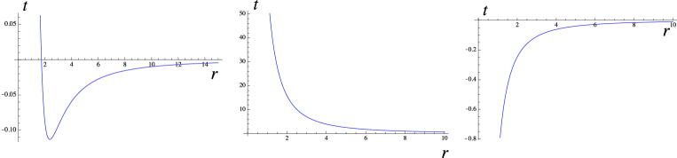
Figure 1: Plots of velocity of light surface $t_{\rm VLS}$ against $r$ for $n=1,2$ with $J^{2/3}>Q$ (left), for $n=3$ with $J^{2/3}>Q$ (middle) and for $J^{2/3}<Q$.

III.4 Scaling limit

Since the event horizon of a black hole is a global concept, it is a difficult task to identify its locus especially in a time-dependent spacetime. Following the previous papers we shall argue the “near-horizon geometry” of the present metric and demonstrate that the null surface of the event-horizon candidate is described by a Killing horizon. By solving null geodesics numerically, we can verify that when $J<Q^{2/3}$ these Killing horizons are indeed event horizons in the original spacetimes. (The reason of the restriction $J<Q^{2/3}$ will be discussed later.)

For convenience, we define dimensionless parameters

$$\tau:=\frac{t_{0}}{Q^{1/2}}\,,\qquad j:=\frac{J}{Q^{3/2}}\,,$$ (80)

and denote dimensionless variables (normalized by $Q$) with tilde, e.g., $\tilde{x}^{\mu}:=Q^{-1/2}x^{\mu}$. Then we can work with the dimensionless metric,

$${\rm d}\tilde{s}^{2}= -f^{2}\left(\tau{\rm d}\tilde{t}+\frac{j}{2\tilde{r}^{2}}\sigma_{3}^{R}\right)^{2}+f^{-1}\left({\rm d}\tilde{r}^{2}+\tilde{r}^{2}{\rm d}\Omega_{3}^{2}\right)\,,$$

$$f= \tilde{r}^{2}\left(\tilde{t}\tilde{r}^{2}+1\right)^{-n/3}\left(\tilde{r}^{2}+1\right)^{(n-3)/3}\,.$$ (81)

The parameter $j$ is the reduced angular momentum and $\tau$ denotes the ratio of energy densities of the scalar fields and the Maxwell fields evaluated on the horizon, respectively MN ; MNII . To simplify the notation, we shall omit tilde in the following.

We have seen in Eq. (51) that the surface $r\to 0$ with $t$ being finite corresponds to the throat infinity. Hence the null surfaces “intersecting” at the throat should be a candidate of future and past horizons. These surfaces are described by the infinite redshift and blueshift surfaces, respectively. We shall focus on the geometry of the very neighborhood of these horizon candidates. The only well-defined “near-horizon” limit is given by

$$t~{}\to~{}\frac{t}{\epsilon^{2}}\,,\qquad r~{}\to~{}\epsilon r\,,\qquad\epsilon~{}\to~{}0\,,$$ (82)

under which the metric is free from the scaling parameter $\epsilon$. The above scaling limit gives rise to the near-horizon geometry, if a horizon exists, the metric of which is given by

$${\rm d}s^{2}_{\rm NH}= -r^{4}\left(tr^{2}+1\right)^{-2n/3}\left(\tau{\rm d}t+\frac{j}{2r^{2}}\sigma_{3}^{R}\right)^{2}$$

$$+r^{-2}\left(tr^{2}+1\right)^{n/3}\left({\rm d}r^{2}+r^{2}{\rm d}\Omega_{3}^{2}\right)\,.$$ (83)

The scalar and gauge fields are also well-defined and given by

$$X_{T}=\frac{1}{3}\left(tr^{2}+1\right)^{1-n/3}\,,\qquad X_{S}=\frac{1}{3}\left(tr^{2}+1\right)^{-n/3}\,,$$ (84)

and

$$A^{(T)}=r^{2}\left(tr^{2}+1\right)^{-1}\left(\tau{\rm d}t+\frac{j}{2r^{2}}\sigma_{3}^{R}\right)\,,$$

$$A^{(S)}=r^{2}\left(\tau{\rm d}t+\frac{j}{2r^{2}}\sigma_{3}^{R}\right)\,.$$ (85)

This spacetime is pseudo-supersymmetric in its own right since it admits a nonvanishing Killing spinor of the form (31) and (32) with $f=r^{2}(tr^{2}+1)^{-n/3}$.

The above near-horizon metric (83) is still time-evolving and spatially inhomogeneous. Nevertheless, as a consequence of the scaling limit (82), the near-horizon metric (83) admits a Killing vector

$$\xi^{\mu}=t\left(\frac{\partial}{\partial t}\right)^{\mu}-\frac{r}{2}\left(\frac{\partial}{\partial r}\right)^{\mu}\,.$$ (86)

It is then convenient to take $\xi^{\mu}$ to be a coordinate vector so that the metric is independent of that coordinate. A possible coordinate choice ($T,R,\psi^{\prime}$) is given by

$$T= \ln|t|+\int^{R}\frac{6R^{6/n-1}(R^{6}-j^{2}){\rm d}R}{n(R^{6/n}-1)\Delta}\,,$$

$$R= (tr^{2}+1)^{n/6}\,,$$

$$\psi^{\prime}= \psi+\int^{R}\frac{12j\tau R^{n/6-1}}{n\Delta}{\rm d}R\,,$$ (87)

where

$$\Delta:= 4R^{4}F(R)+j^{2}\,,$$

$$F(R):= \tau^{2}R^{-4}(R^{6/n}-1)^{2}-\frac{1}{4}R^{2}\,,$$ (88)

In this new coordinate system, the Killing field is simply given by $\xi^{\mu}=(\partial/\partial T)^{\mu}$, as we desired. After some algebra the near-horizon metric (83) is cast into an apparently stationary form,

$${\rm d}s^{2}_{\rm NH}= -F(R)\left[{\rm d}T+\frac{j\tau(R^{6/n}-1)}{2R^{4}F(R)}{\sigma_{3}^{\prime}}^{R}\right]^{2}+\frac{j^{2}R^{2}({\sigma_{3}^{\prime}}^{R})^{2}}{16F(R)}$$

$$+\frac{36\tau^{2}R^{12/n}{\rm d}R^{2}}{n^{2}\Delta}+\frac{R^{2}}{4}\left[(\sigma_{1}^{R})^{2}+(\sigma_{2}^{R})^{2}+({\sigma_{3}^{\prime}}^{R})^{2}\right]\,.$$ (89)

Here, ${\sigma_{3}^{\prime}}^{R}={\rm d}\psi^{\prime}+\cos\theta{\rm d}\phi$. Although its asymptotic structure is highly nontrivial, it is easy to recognize that this spacetime has Killing horizons (if any) at $\Delta=0$. The Killing horizon is generated by a linear combination of stationary and angular Killing vectors,

$$\zeta=\frac{\partial}{\partial T}+2\Omega_{h}\frac{\partial}{\partial\psi^{\prime}}\,,$$ (90)

where

$$\Omega_{h}=\left.\frac{j}{2\sqrt{R^{6}-j^{2}}}\right|_{\rm horizon}\,.$$ (91)

Here, $\Omega_{h}$ is the angular velocity of the horizon (associated with $2\partial/\partial\psi^{\prime}=\partial/\partial\phi_{2}+\partial/\partial{\phi_{1}}$). The horizon angular velocity $\Omega_{h}$ is constant anywhere on the horizon, which is a generic feature of a Killing horizon Carter . Contrary to (truly) supersymmetric black holes, the angular velocity of the horizon is nonvanishing, i.e., the horizon is rotating. In other words, the generator of the event horizon of a supersymmetric black hole is tangent to the stationary Killing field at infinity. Equation (90) shows that $\partial/\partial t$ is not the generator of the event horizon. This is a distinguished property not shared by the BPS black holes.

Since $\Delta$ fails to have a double root in general, it follows that the horizon is not extremal unless parameters $(\tau,j)$ are fine-tuned. The reason of the appearance of the “throat” geometry at $r\to 0$ lies in the fact that $(t,r)$-coordinates cover the “white-hole region” as well as the outside region of a black hole (see Figure 5 in MNII ).

Equations (84) and (87) imply that the values of scalar fields $X_{I}$ on the horizon are determined by the horizon radius, which is expressed in terms of the charge $Q$, (inverse of) potential height $t_{0}$ and the angular momentum $j$. This situation is closely analogous to the attractor mechanism attractor , according to which the values of scalar fields on the horizon are expressed by charges and independent of the asymptotic values of the scalar fields at infinity. But as it stands it appears hard to say whether such a mechanism always works in the time-dependent case.

In the following subsections we shall clarify various physical features of the near-horizon metric (89).

III.4.1 Horizons

The loci of Killing horizons $\Delta=0$ can be classified according to the values of $\tau$ and $j^{2}$. We shall say “under-rotating” when the spacetime (83) admits horizons. Otherwise it is said to be “over-rotating.” The quantity $R_{-}$ will be consistently used when $\Delta>0$ for $R<R_{-}$.

(i) $n=1$. When the angular momentum parameter $|j|$ is less than the critical value $j_{(1)}$, i.e.,

$$j^{2}<j_{(1)}^{2}:=\frac{1+16\tau^{2}}{16\tau^{2}}\,,$$ (92)

the near-horizon spacetime admits two horizons,

$$R_{\pm}^{6}=\frac{1+8\tau^{2}\pm\sqrt{1+16\tau^{2}(1-j^{2})}}{8\tau^{2}}\,.$$ (93)

For the over-rotating case $j^{2}>j_{(1)}^{2}$, there exist no horizons. We find the similar results for the case of non-integer values of $n<2$.

(ii) $n=2$. This case is further categorized into the following three cases.

1. $0<\tau<1/2$. For any values of $j$, a single horizon occurs at

   $$R_{-}^{3}=\frac{\sqrt{4\tau^{2}+(1-4\tau^{2})j^{2}}-4\tau^{2}}{1-4\tau^{2}}\,.$$ (94)

2. $\tau=1/2$. For any values of $j$, a single horizon occurs at

   $$R_{-}^{3}=\frac{1+j^{2}}{2}\,.$$ (95)

3. $\tau>1/2$. When the angular momentum parameter $|j|$ is less than the critical value $j_{(2)}$, i.e.,

   $$j^{2}<j_{(2)}^{2}:=\frac{4\tau^{2}}{4\tau^{2}-1}\,,$$ (96)

   two horizons exist at

   $$R_{\pm}^{3}=\frac{4\tau^{2}\pm\sqrt{4\tau^{2}-(4\tau^{2}-1)j^{2}}}{4\tau^{2}-1}\,.$$ (97)

   For the over-rotating case $j^{2}>j^{2}_{(2)}$, no horizons develop.

(iii) $n=3$. In this case, the metric (89) is not the “near-horizon” geometry, but is the original metric itself written in the stationary coordinates. This metric describes a charged rotating black hole in de Sitter space derived by Klemm and Sabra Klemm:2000vn . Let us discuss its horizon structure in detail.

There exists at least one horizon corresponding to the cosmological horizon. For $\tau\leq\sqrt{3/2}$ there appears only a cosmological horizon $R_{c}$. For $\tau>\sqrt{3/2}$, the number of horizons depend on the value of $j^{2}$. Three distinct horizons ($R_{-}<R_{+}<R_{c}$) exist for $j^{2}_{(3)-}<j^{2}<j^{2}_{(3)+}$, where

$$j^{2}_{(3)\pm} :=\frac{4\tau^{2}}{27}\left[\pm 8\sqrt{2}\tau(2\tau^{2}-3)^{3/2}\right.$$

$$\left.~{}~{}~{}~{}~{}~{}~{}~{}~{}~{}-32\tau^{4}+9(8\tau^{2}-3)\right]\,.$$ (98)

For $j^{2}=j^{2}_{(3)+}$, inner and outer black-hole horizons are degenerate. While, for $j^{2}=j^{2}_{(3)-}$ the outer black-hole horizon and the cosmological horizon are degenerate. $j^{2}_{(3)-}$ takes real positive values for $\sqrt{3/2}<\tau<3\sqrt{3}/4$, otherwise the inner horizon does not exist.

A simple calculation reveals that the spacetime (83) is regular on and outside the Killing horizon (if any). Only the existing curvature singularity is at $R=0$. It is almost clear to construct the local coordinate systems that pass through the Killing horizon $\Delta=0$.

In hindsight, we can understand why the horizon in the present spacetime is not extremal as follows. In the case of the time-independent (truly) BPS solutions such as a BMPV black hole, the Killing horizon lies at $f=0$ since $V^{\mu}=(\partial/\partial t)^{\mu}$ is an everywhere causal Killing field constructed by a Killing spinor $\epsilon$ as $V^{\mu}=i\bar{\epsilon}\gamma^{\mu}\epsilon$ (see GGHPR ). For the present time-dependent pseudo-supersymmetric black hole, on the other hand, the vector field $V^{\mu}=(\partial/\partial t)^{\mu}$ is not the Killing-horizon generator: the horizon is generated by $\xi^{\mu}=t(\partial/\partial t)^{\mu}-(r/2)(\partial/\partial r)^{\mu}+\Omega_{h}(\partial/\partial\psi)^{\mu}$ given in Eq. (90). The vector field $V^{\mu}$ does not give rise to any (asymptotic) symmetry.

Physically speaking, the degeneracy of the horizon is broken by introducing of the time-dependent scalar fields (which do not contribute to the total mass when the spacetime is stationary) or the positive cosmological constant. These ingredients destroy the fine balance between the mass energy and the charges. When the rotation is also added the centrifugal force gives a negative contribution to the mass energy $M\to M-J^{2}$–which takes place only in $D=5$ as discussed before–thus it exceeds the extremal threshold value if the rotation becomes too large.

III.4.2 Ergoregion

An obvious major difference from our previous non-rotating solutions MN ; MNII is that the near-horizon metric possesses the ergosurface at $F(R)=0$. Since $\Delta>4R^{4}F(R)$, the ergosurface lies strictly outside the horizon, contrary to the 4-dimensional Kerr black hole for which the ergosurface touches the horizon at the rotation axis.

When the rotating vanishes ($j=0$), the roots of $F=0$ correspond to the loci of horizons MN ; MNII . Since $\Delta=0$ reduces to $F(R)=0$ when $j=0$, the explicit expression of the ergosphere is given by setting $j=0$ of the horizon radius. For $n=1,2$ they are given by Eqs. (93), (94), (95) and (97) with $j=0$. Note, however, that since the asymptotic structures are quite peculiar when $n=1,2$, there may arise an ambiguity concerning the definition of the energy . It may therefore equivocal whether $R_{\rm erg}$ has a definitive meaning in the $n=1,2$ cases.

When $n=3$ the asymptotic region is described by de Sitter space, so that we can use the standard time translation with respect to the observer at the cosmological horizon to define the energy. Hence the notion of ergoregion is meaningful in this sense. There exist three distinct roots, $R_{\rm erg,-}<R_{\rm erg,+}<R_{\rm erg,c}$, for $\tau>\tau_{\rm cr}:=3\sqrt{3}/4$, two roots for $\tau=\tau_{\rm cr}$ and a single root $R_{\rm erg,-}$ for $\tau<\tau_{\rm cr}$.

The ergoregion does not arise for the supersymmetric black hole, which inevitably forbids the ergoregion inside which the stationary Killing field becomes spacelike. The ergoregion is intrinsic to a rotating black hole and allows particles to have a negative energy. This means that the rotation energy of a black hole can be subtracted via the Penrose process and the superradiant scattering process. We shall demonstrate in Appendix B that this is indeed the case for the $n=3$ Klemm-Sabra solution.

III.4.3 Closed timelike curves

Write the near-horizon metric (89) as

$${\rm d}s_{\rm NH}^{2}=-\frac{\Delta}{4R^{4}\varDelta_{L}}{\rm d}T^{2}+\frac{36\tau^{2}R^{12/n}{\rm d}R^{2}}{n^{2}\Delta}+\frac{R^{2}}{4}\left[(\sigma_{1}^{R})^{2}+(\sigma_{2}^{R})^{2}+\varDelta_{L}\left({\sigma_{3}^{\prime}}^{R}-\frac{2j\tau(R^{6/n}-1)}{R^{6}\varDelta_{L}}{\rm d}T\right)^{2}\right]\,,$$ (99)

where we have also used $\varDelta_{L}$ as the near-horizon limit of (75):

$$\varDelta_{L}=1-\frac{j^{2}}{R^{6}}\,.$$ (100)

Consequently the Hopf fibres become timelike inside the VLS ($\varDelta_{L}<0$), viz, the near-horizon metric (89) is also causally unsound. In terms of $\varDelta_{L}$, $\Delta$ is

$$\Delta=4\tau^{2}(R^{6/n}-1)^{2}-R^{6}\varDelta_{L}\,.$$ (101)

It follows that the event horizon ($\Delta=0$) is outside the VLS Matsuno:2007ts . Hence the causality violating region is always hidden behind the horizon ($R_{L}<R_{+}$) in the near-horizon geometry (89) . On the other hand, it is naked in the over-rotating case where the horizon does not exist. This should be contrasted with the BMPV or asymptotically AdS ($\mathfrak{g}\in\mathbb{R}$) Klemm-Sabra black hole. In the former case the VLS is outside the event horizon if the angular momentum is large $J>Q^{2/3}$. In the latter case a naked time machine inevitably appears outside the event horizon. However, it allows no geodesics to penetrate, so that the horizon exterior is geodesically complete. In the present case the area of the horizon is given by

$${\rm Area} =2\pi^{2}R^{3}\left.\sqrt{\varDelta_{L}}\right|_{\rm horizon}=4\pi^{2}\tau(R_{+}^{6/n}-1)\,.$$ (102)

which always makes sense contrary to the BMPV or the asymptotically AdS Klemm-Sabra black hole: the latter two spacetimes have an “imaginary horizon area” in the over-rotating case. These formal horizons in the over-rotating case are “repulsons” into which no freely falling orbits penetrate (see e.g., GibbonsBMPV ; Caldarelli:2001iq ; Herdeiro:2000ap ; Dyson:2006ia ).

III.4.4 Geodesic motions

It is illustrative to consider geodesics in the near-horizon metric (89). For $n=3$, the following analysis yields the geodesic motion in the exact Klemm-Sabra geometry, not restricted in the neighborhood of its horizons. The particle motion in asymptotically AdS Klemm-Sabra solution ($\mathfrak{g}\in\mathbb{R}$) was previously examined in Caldarelli:2001iq . Although the behavior of the particle motion in asymptotically de Sitter case is of course considerably different from that case, the technical method is similar. The analysis in this subsection unveils that the horizon can be reached within a finite affine time from outside.

The Hamilton-Jacobi equation in the near-horizon geometry (89) reads

$$-\frac{\partial S}{\partial\lambda}=\frac{1}{2}g^{\mu\nu}_{\rm NH}\left(\frac{\partial S}{\partial x^{\mu}}\right)\left(\frac{\partial S}{\partial x^{\nu}}\right)\,,$$ (103)

where the right-hand side of this equation defines a geodesic Hamiltonian and $\lambda$ is an affine parameter. Assume the separable form of Hamilton’s principal function,

$$S= \frac{1}{2}m^{2}\lambda-ET+L_{L}\phi+L_{R}\psi^{\prime}+S_{R}(R)+S_{\theta}(\theta)\,,$$ (104)

where $E,L_{R},L_{L}$ and $m$ are constants of motion corresponding to energy, right-rotation, left-rotation and rest mass of a particle. Since the near-horizon metric keeps the ${\rm U}(2)$-symmetry, there exists a reducible Killing tensor of the form (71), which reads in the coordinates (89) as

$$K_{\mu\nu}{\rm d}x^{\mu}{\rm d}x^{\nu}= \left[\frac{j\tau}{2R^{4}}(R^{6/n}-1){\rm d}T-\frac{R^{2}\varDelta_{L}}{4}({\sigma^{\prime}_{3}}^{R})\right]^{2}$$

$$+\frac{R^{4}}{16}\left[(\sigma_{1}^{R})^{2}+(\sigma_{2}^{R})^{2}\right]\,.$$ (105)

Accordingly, besides obvious constants of motion ($E,L_{R},L_{L},m$) generated by Killing vectors, we have an additional integration constant $L^{2}$ with dimensions of angular momentum squared such that

$$L^{2}:=\sum_{i}(\xi^{R}_{i}S)^{2}\,.$$ (106)

This constant of motion enables us to separate the variables as

$$\left(\frac{{\rm d}}{{\rm d}\theta}S_{\theta}\right)^{2}+\frac{1}{\sin^{2}\theta}\left(L_{L}^{2}+L_{R}^{2}-2\cos\theta L_{R}L_{L}\right)=L^{2}\,.$$ (107)

The constant $L^{2}$ represents the left and right Casimir invariant of the ${\rm SU}(2)$ subgroup of ${\rm SO}(4)$ rotation group. These two Casimirs turn out to be the same for the scalar representation. It follows that the particle motion and the scalar-field equation are Liouville-integrable. The governing equations are obtainable by differentiating the principal function (104) by corresponding constants of motion. Using the relation for angular variable (107), we obtain a set of useful 1st-order equations

$$\frac{{\rm d}R}{{\rm d}\lambda} =\pm\frac{n\sqrt{\Delta}}{6\tau R^{6/n}}\left[\frac{E}{F}-m^{2}-\frac{4(L^{2}-L_{R}^{2})}{R^{2}}-\frac{16R^{2}F}{\Delta}\left(L_{R}+\frac{j\tau(R^{6/n}-1)E}{2R^{4}F}\right)^{2}\right]^{1/2}\,,$$ (108)

$$\frac{{\rm d}\theta}{{\rm d}\lambda} =\pm\frac{4}{R^{2}}\left[L^{2}-\frac{1}{\sin^{2}\theta}\left(L_{L}^{2}+L_{R}^{2}-2\cos\theta L_{R}L_{L}\right)\right]^{1/2}\,,$$ (109)

$$\frac{{\rm d}T}{{\rm d}\lambda} =\frac{4R^{4}\varDelta_{L}}{\Delta}E-\frac{8j\tau(R^{6/n}-1)L_{R}}{\Delta R^{2}}\,,$$ (110)

$$\frac{{\rm d}\phi}{{\rm d}\lambda} =\frac{4}{R^{2}\sin^{2}\theta}(L_{L}-L_{R}\cos\theta)\,,$$ (111)

$$\frac{{\rm d}\psi^{\prime}}{{\rm d}\lambda} =\frac{4(L_{R}-L_{L}\cos\theta)}{R^{2}\sin^{2}\theta}-\frac{4}{R^{2}\Delta}\left[j^{2}L_{R}-2j\tau(R^{6/n}-1)E\right]\,.$$ (112)

If there are no angular momenta of a particle ($L=L_{R}=L_{L}=0$), one sees that there is no motion in directions $\theta$ and $\phi$, but there is a nonvanishing motion along $\psi^{\prime}$, encoding the frame dragging due to the black-hole rotation.

By virtue of high degree of symmetries, the problem reduces to the one dimensional radial equation (108), which is arranged to give

$$\left(\frac{{\rm d}R}{{\rm d}\lambda}\right)^{2}= \frac{n^{2}}{9\tau^{2}R^{4(3/n-1)}}\biggl{[}\varDelta_{L}(E-2\Omega L_{R})^{2}$$

$$-\frac{j^{2}L_{R}^{2}\Delta}{R^{12}\varDelta_{L}}-\Delta\left(\frac{L^{2}}{R^{6}}+\frac{m^{2}}{4R^{4}}\right)\biggl{]}\,,$$ (113)

$$= \frac{n^{2}\varDelta_{L}}{9\tau^{2}R^{4(3/n-1)}}(E-V^{+})(E-V^{-})\,,$$ (114)

where $\Omega$ and $V^{\pm}$ are the angular velocity of a locally nonrotating observer and the effective potentials, which are defined by

$$\Omega:= \frac{j\tau(R^{6/n}-1)}{R^{6}\varDelta_{L}}\,,$$ (115)

$$V^{\pm}:= 2\Omega L_{R}\pm\frac{\sqrt{\Delta\left[j^{2}L_{R}^{2}+\varDelta_{L}R^{6}\left(L^{2}+{m^{2}R^{2}}/4\right)\right]}}{\varDelta_{L}R^{6}}\,.$$ (116)

The allowed region is $E>V^{+}$ or $E<V^{-}$ for $\varDelta_{L}>0$, whereas it is ${\rm min}[V^{\pm}]<E<{\rm max}[V^{\pm}]$ for $\varDelta_{L}<0$.

Equation (110) becomes

$$\frac{{\rm d}T}{{\rm d}\lambda}=\frac{4R^{4}\varDelta_{L}}{\Delta}\left(E-2\Omega L_{R}\right)\,.$$ (117)

When $\Delta>0$ and $\varDelta_{L}>0$, $E>V^{0}:=2\Omega L_{R}$ follows. Thus, $E$ must be positive for a particle with $\Omega L_{R}>0$ moving forwards with respect to the time coordinate $T$. Inside the VLS ($\varDelta_{L}<0$) where $\Delta>0$, a particle with $E>V^{0}$ moves backwards with respect to the coordinate $T$. One also verifies that the horizon $\Delta=0$ is an infinite redshift surface for the time coordinate $T$, which is of course a coordinate artifact.

From (106) one finds $L^{2}\geq L_{R}^{2}$. When the equality holds, $L_{L}=0$ is satisfied. Thus Eq. (107) implies that the particle motion is confined on the equatorial plane $\theta=\pi/2$ and Eq. (111) implies $\phi={\rm constant}$. The same remark applies to the original metric (52) since this assertion only comes from the ${\rm U}(2)$-symmetries of the solution.

It is clear from Eq. (113) that massless particles with $L=L_{R}=0$ cannot cross the VLS. In the over-rotating case, the geodesics with $L_{R}=0$ cannot cross the VLS either, since the right-hand side of (113) becomes negative before the VLS is reached.

In the case of $L_{R}\neq 0$, it is dependent on the parameters whether the geodesic particle moving forwards can cross the VLS or not. When $j<1$, $\Omega L_{R}$ diverges positively (negatively) as $R\to R_{L}+0$ for the particle having the opposite (same) spin as the black hole. Hence the particle with opposite angular momentum ($jL_{R}<0$) cannot penetrate the VLS for $j<1$. Similarly, when $j>1$ $\Omega L_{R}$ diverges positively (negatively) as $R\to R_{L}+0$ for the particle having the same (opposite) spin as the black hole. Thus the particle with $j>1$ never penetrate the VLS when it has the same spin as the hole $jL_{R}>0$.

Though causal geodesics may cross the VLS, it is shown that they never encounter the singularity at $R=0$ at least for $n=2,3$. For $L>|L_{R}|$, the function inside the square-root of $V^{\pm}$ (116) becomes negative around $R=0$, so that $V^{\pm}$ does not exist around $R=0$ and has a confluent point inside the VLS, which prohibits geodesics to enter inside. For $L=|L_{R}|$, it can be easily shown that $V^{+}<V^{0}<V^{-}$ holds around $R=0$ and they take value $2\tau L_{R}/j$ at $R=0$. It follows that geodesics with $E=2\tau L_{R}/j$ may reach $R=0$. For $n=1$ this is indeed the case. By contrast, for $n=2,3$ ${\rm d}V^{0}/{\rm d}R<(>)0$ holds around $R=0$ for $jL_{R}>(<)0$, which forbids the geodesics to hit the singularity since $E<V^{0}$ and $V^{+}<E<V^{-}$ are the allowed region for the future-pointing particles. Accordingly, the singularity $R=0$ has a repulsive nature. We can expect that geodesics rarely reach the singularity also in the dynamical settings.

III.5 Global structure

We are now ready to discuss the global structures of the time-dependent and rotating spacetime (52). The most useful visualization of the causal structure of a spacetime is the conformal diagram. To this end it is necessary to find a two-dimensional (totally geodesic) integrable submanifold. Now the spacetime is regarded as an $\mathbb{R}^{2}$ bundle over $S^{3}$. Unfortunately, the distribution spanned by $\partial/\partial t$ and $\partial/\partial r$ is not integrable, forbidding us to have a foliation by a two-dimensional conformal diagram. The frame-dragging effect inevitably drives the $\psi$-motion.

Nevertheless, the two-dimensional metric

$${\rm d}s_{2}^{2}=-\frac{\tau^{2}f^{2}}{\Delta_{L}}{\rm d}t^{2}+\frac{{\rm d}r^{2}}{f}\,,$$ (118)

still contains some information about the spacetime structure and gives us useful visualization . The above metric (118) is associated with the null geodesics with $\theta=\pi/2$ and $\phi={\rm constant}$ corresponding to $L=L_{R}=L_{L}=0$: hence they cannot penetrate the VLS, which is found to be a timelike or null surface. As in the BMPV case, the 2-dimensional metric (118) is not Lorentzian inside the VLS.

From the analysis of the previous subsection, we found that the original time-independent metric (89) admits Killing horizons at $\Delta=0$. In the non-rotating case ($j=0$), the null surfaces $r=0$ with $t=\pm\infty$ are Killing horizons also for the original spacetime MNII , since the Killing vector is parallel to the generators of horizons.

When a rotation is present we must be careful. Now there exists a VLS (77), which is bounded below when $j>1$ (see left and middle plots in figure 1), so that the past horizon $t\to-\infty$ may not exist (since we are focusing on the 2-dimensional metric (118), no causal geodesics penetrate the VLS: inside the VLS is not the physical region of spacetime). Even if the near-horizon metric MNII admits some Killing horizons, we cannot immediately conclude that they are also Killing horizons in the original metric.

The analysis of singularities, asymptotic infinity, behaviors of VLS (figure 1) and the near-horizon geometries have provided us sufficient information to deduce Carter-Penrose diagrams. As a striking confirmation we have solved the geodesic equations numerically and obtained the conformal diagrams displayed in figure 2, which may be summarized as follows (we have excluded the special case of the degenerate horizons).

(i) $n=1$. The asymptotic region is approximated by an FLRW universe obeying a decelerating expansion $a=(\bar{t}/\bar{t}_{0})^{1/4}$ caused by a massless scalar field. Then the null infinity $\mbox{$\mathscr{I}$}^{-}$ possesses an ingoing null structure. When $j<j_{(1)}$, two Killing horizons $R_{\pm}$ arise (93). Since the VLS diverges negatively as $r\to 0$ when $j<1$ (right plots in figure 1), the conformal diagram is (I). Even if two horizons exist in the near-horizon geometry for $1<j<j_{(1)}$, the VLS conceals the past horizon $R_{-}$ (corresponding to $t\to-\infty$) since the VLS diverges positively as $r\to$ (left plots in figure 2). Then diagram (II) is obtained. Note that the $R_{-}={\rm constant}$ surface asymptotically approaches null as $t\to\infty$, and $R_{L}$ is timelike almost everywhere (it happens to be null precisely at one point). For the over-rotation $j>j_{(1)}$, no Killing horizons arise. Hence the conformal diagram is (V).

(ii) $n=2$. The spacetime approaches to the marginally accelerating universe, expanding linearly with cosmic time $a=\bar{t}/\bar{t}_{0}$. This is caused by the fluid with equations of state $P=-\rho/2$. For $\tau>1/2$ there exists two Killing horizons (93), so that conformal diagram is the same as case (i); it is (I) for $0<j<1$, (II) for $1<j<j_{(2)}$ and (V) for $j>j_{(2)}$. An essential difference from the $n=1$ case arises when $\tau\leq 1/2$, in which case there exists an internal null infinity $\mbox{$\mathscr{I}$}^{+}_{\rm in}$ where $R\to\infty$ with $r\to 0$ and $t\to\infty$. Only ingoing null particles can get to $\mbox{$\mathscr{I}$}^{+}_{\rm in}$. The existence of internal null infinity can be shown by solving the geodesics asymptotically as in 4-dimensions MNII . It follows that conformal diagrams for $\tau\leq 1/2$ are (III) when $j<1$ and (IV) when $j>1$.

(iii) $n=3$. The conformal diagrams are similar to the Kerr-de Sitter spacetime. Infinity $\mbox{$\mathscr{I}$}^{+}$ consists of a spacelike slice due to the acceleration of the universe. First, consider the case in which the near-horizon metric (89) admits three distinct horizons $R_{\pm}$ and $R_{c}$. This occurs when $\sqrt{3/2}<\tau<3\sqrt{3}/4$ with $j_{(3)-}<j<j_{(3)+}$ and $\tau>3\sqrt{3}/4$ with $(0\leq)j<j_{(3)+}$. Taking into account the fact that for $j<1$ the VLS $t_{\rm VLS}(r)$ diverges negatively as $r\to 0$, which removes past horizons ($t\to-\infty$ and $r\to 0$ with $tr^{2}$ finite) in the near-horizon geometry (83). Therefore when $\tau>3\sqrt{3}/4$ with $(0\leq)j<1$ the conformal diagram is (VI), whereas it is (VI’) when $1<j<j_{(3)+}$ with $\tau>3\sqrt{3}/4$, or $(1<)j_{(3)-}<j<j_{(3)+}$ with $\sqrt{3/2}<\tau<3\sqrt{3}/4$. These two are essentially the same: they constitute the different coordinate patches depending on the value of $j$. In (V’) the slice $t=0$ and $r\to\infty$ with $tr^{2}$ finite comprises a null boundary. When there appears only a cosmological horizon $R_{c}$ (i.e., $\tau<\sqrt{3/2}$, $\sqrt{3/2}<\tau<3\sqrt{3}/4$ with $j<j_{(3)-}$ or $j>j_{(3)+}$ and $\tau>3\sqrt{3}/4$ with $j>j_{(3)+}$), the spacetime diagram is (VII) for $j<1$ and (VII’) otherwise. Again, (VII) and (VII’) are essentially identical. In (VII’) the slice $t=0$ and $r\to\infty$ with $tr^{2}$ finite is also a null surface.

To summarize, the cases (I), (II), (VI) and (VI’) correspond to the rotating black-hole geometry.

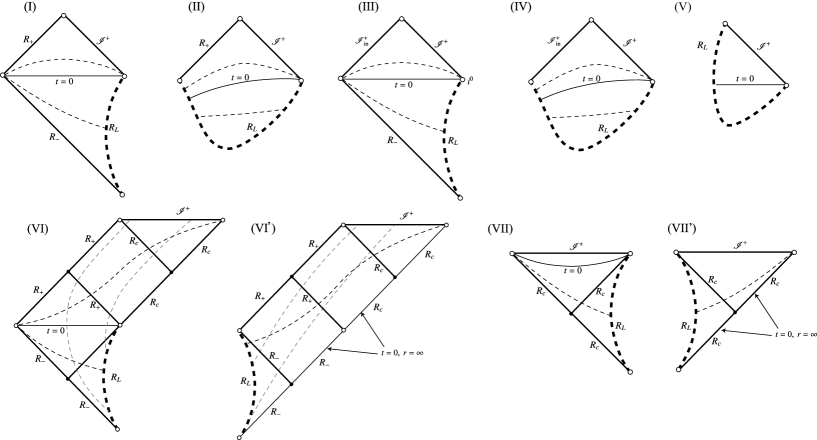
Figure 2: Conformal diagrams of the 2-dimensional spacetime (118), by which null geodesics with zero angular momentum is described. $R_{+}$, $R_{-}$ and $R_{c}$ are all Killing horizons corresponding respectively to the black-hole event horizon, the white-hole horizon and the cosmological horizon. The thick dotted curves represent the VLS. Thin black and gray dotted curves are $t={\rm constant}$ and $r={\rm constant}$ surfaces, respectively. White and black circle are infinities (including throat) and bifurcation surfaces. Since the 2-dimensional metric (118) becomes Riemannian inside the VLS, the diagrams come to an end at $R_{L}$. Remark that we are formally writing the 2-dimensional figures, there still remains the angular motion because of the frame dragging: these figures do not display all the causal information. Though these diagrams are restricted to the $r^{2}>0$ region, the spacetime can be extended across the null surfaces $R_{\pm}$ and $R_{c}$, which are nothing but the ordinary chart boundaries. The conformal diagrams are (I) for $n=1$ with $j<1$, and for $n=2$ with $j<1$ and $\tau>1/2$, (II) for $n=1$ with $1<j<j_{(1)}$, and for $n=2$ with $1<j<j_{(2)}$ and $\tau>1/2$, (III) for $n=2$ with $\tau\leq 1/2$ and $j<1$, (IV) for $n=2$ with $\tau\leq 1/2$ and $j>1$, (V) for $n=1$ with $j>j_{(1)}$ and for $n=2$ with $\tau>1/2$ and $j>j_{(2)}$, whereas diagrams (VI)–(VII’) correspond to $n=3$: (VI) for $\tau>3\sqrt{3}/4$ with $j<1$, (VI’) for $\tau>3\sqrt{3}/4$ with $1<j<j_{(3)+}$, and for $\sqrt{3/2}<\tau<3\sqrt{3}/4$ with $j_{(3)-}<j<j_{(3)+}$, (VII) for $\tau<\sqrt{3/2}$ with $j<1$ and for $\sqrt{3/2}<\tau<3\sqrt{3}/4$ with $j<1$, and (VII’) for $\tau<\sqrt{3/2}$ with $j>1$, for $\sqrt{3/2}<\tau<3\sqrt{3}/4$ with $1<j<j_{(3)-}$ or $j>j_{(3)+}$ and for $\tau>3\sqrt{3}/4$ with $j>j_{(3)+}$.

IV Dimensional oxidization and reduction

In the previous sections, some black hole solutions in the STU theory have been elaborated in the framework of the 5-dimensional theory. We shall discuss in this section the liftup and compactification procedure to other number of dimensions.

IV.1 Lift up to M-theory

The time-evolving and spatially-inhomogeneous solutions in 4- and 5- dimensions were originally derived from the dimensional reduction of intersecting M-branes in 11-dimensional supergravity. Now we argue the solutions of case (ii)–where two of $V_{I}$’s vanish–can be embedded in 11-dimensional supergravity.

The 11-dimensional supergravity action is given by

$$S_{11}=\frac{1}{2\kappa_{11}^{2}}\int\left({}^{11}R\star_{11}1-\frac{1}{2}{\mbox{$\mathcal{F}$}}\wedge\star_{11}{\mbox{$\mathcal{F}$}}-\frac{1}{6}\mbox{$\mathcal{A}$}\wedge\mbox{$\mathcal{F}$}\wedge\mbox{$\mathcal{F}$}\right)\,,$$ (119)

where $\mbox{$\mathcal{F}$}={\rm d}\mbox{$\mathcal{A}$}$ is the 4-form field strength. The equations of motion are Einstein’s equations,

$${}^{11}R_{AB}-\frac{1}{2}{}^{11}Rg_{AB}= \frac{1}{2\cdot 3!}\left(\mbox{$\mathcal{F}$}_{ACDE}{\mbox{$\mathcal{F}$}_{B}}^{CDE}\right.$$

$$\left.-\frac{1}{8}g_{AB}\mbox{$\mathcal{F}$}_{CDEF}\mbox{$\mathcal{F}$}^{CDEF}\right)\,,$$ (120)

and the gauge-field equations

$${\rm d}\star_{11}\mbox{$\mathcal{F}$}+\frac{1}{2}\mbox{$\mathcal{F}$}\wedge\mbox{$\mathcal{F}$} =0\,.$$ (121)

In this section $A,B,...$ denote the 11-dimensional indices.

Let us consider the “intersecting M2/M2/M2 metric” of the following form Elvang:2004ds ,

$${\rm d}s_{11}^{2}= {\rm d}s_{5}^{2}+X^{1}\left({\rm d}y_{1}^{2}+{\rm d}y_{2}^{2}\right)+X^{2}\left({\rm d}y_{3}^{2}+{\rm d}y_{4}^{2}\right)$$

$$+X^{3}\left({\rm d}y_{5}^{2}+{\rm d}y_{6}^{2}\right)\,,$$ (122)

$$\mbox{$\mathcal{A}$}= A^{(1)}\wedge{\rm d}y_{1}\wedge{\rm d}y_{2}+A^{(2)}\wedge{\rm d}y_{3}\wedge{\rm d}y_{4}$$

$$+A^{(3)}\wedge{\rm d}y_{5}\wedge{\rm d}y_{6}\,,$$ (123)

where the metric is independent of the brane coordinates $y_{1},...,y_{6}$. This solution is specified by 5-dimensional metric,

$${\rm d}s_{5}^{2}= -\left(H_{1}H_{2}H_{3}\right)^{-2/3}\left({\rm d}t+\omega\right)^{2}$$

$$+\left(H_{1}H_{2}H_{3}\right)^{1/3}h_{mn}{\rm d}x^{m}{\rm d}x^{n}\,,$$ (124)

as well as three scalars $X^{I}~{}(I=1,2,3)$ and three one-forms $A^{(I)}$ which are given by

$$A^{(I)}= H_{I}^{-1}\left({\rm d}t+\omega\right)\,,\qquad X^{I}=H_{I}^{-1}\left(H_{1}H_{2}H_{3}\right)^{1/3}\,.$$ (125)

Here, $h_{mn}$ is the metric on the 4-dimensional base space. $\omega=\omega_{m}{\rm d}x^{m}$ is viewed as a one-form on the base space, i.e., $\omega_{\mu}V^{\mu}=0$ where $V^{\mu}=(\partial/\partial t)^{\mu}$.

Since the metric ansatz (124) is independent of the coordinates $y_{1},...,y_{6}$, the solution can be dimensionally reduced to 5-dimensions. Noting that the six-torus ${T}^{6}$ has a constant volume $X^{1}X^{2}X^{3}=1$, it turns out that the 5-dimensional metric ${\rm d}s_{5}^{2}$ is the 5-dimensional Einstein-frame metric. Thus, the metric ansatz (122) gives the 5-dimensional action of gravity sector as

$$S_{g} =\frac{1}{2\kappa_{5}^{2}}\int{\rm d}^{5}x\sqrt{-g_{5}}\left[{}^{5}R-\frac{1}{2}\sum_{I}(\nabla^{\mu}\ln X^{I})(\nabla_{\mu}\ln X^{I})\right]\,,$$ (126)

where we have used $X^{1}X^{2}X^{3}=1$. We can proceed the form field sector analogously. Letting $F^{(I)}:={\rm d}A^{(I)}$ denote the two-form field strengths, we find

$$\mbox{$\mathcal{F}$}_{ABCD}\mbox{$\mathcal{F}$}^{ABCD}=12\sum_{I}(X^{I})^{-2}F^{(I)}_{\mu\nu}F^{(I)\mu\nu}\,,$$ (127)

$$\mbox{$\mathcal{A}$}\wedge\mbox{$\mathcal{F}$}\wedge\mbox{$\mathcal{F}$}=2\left(A^{(1)}\wedge F^{(2)}\wedge F^{(3)}+A^{(2)}\wedge F^{(3)}\wedge F^{(1)}\right.$$

$$\qquad\qquad\qquad\left.+A^{(3)}\wedge F^{(1)}\wedge F^{(3)}\right)\wedge{\rm Vol}(T^{6})\,,$$ (128)

then the Lagrangian for the gauge fields reads

$$S_{F}=\frac{1}{2\kappa_{5}^{2}}\int{\rm d}^{5}x\sqrt{-g_{5}}\left[-\frac{1}{4}\sum_{I}(X^{I})^{-2}F^{(I)}_{\mu\nu}F^{(I)\mu\nu}+\frac{1}{12}\epsilon^{\mu\nu\rho\sigma\tau}\left(A^{(1)}_{\mu}F^{(2)}_{\nu\rho}F^{(3)}_{\sigma\tau}+A^{(2)}_{\mu}F^{(3)}_{\nu\rho}F^{(1)}_{\sigma\tau}+A^{(3)}_{\mu}F^{(1)}_{\nu\rho}F^{(2)}_{\sigma\tau}\right)\right]\,,$$ (129)

where $\epsilon_{\mu\nu\rho\sigma\tau}$ is the volume-element compatible with the 5-dimensional metric ${\rm d}s^{2}_{5}$ and $\kappa_{5}^{2}:=\kappa_{11}^{2}/{\rm Vol}(T^{6})$. It follows that the reduced action $S_{5}=S_{g}+S_{F}$ exactly coincides with that of the STU-theory; the 5-dimensional minimal ungauged ($\mathfrak{g}=0$) ${\rm U}(1)^{3}$-supergravity (1) with the metric of the potential space given by

$$G_{IJ}=\frac{1}{2}{\rm diag}\left[(X^{1})^{-2},(X^{2})^{-2},(X^{3})^{-2}\right]\,,$$ (130)

and the constants $C_{IJK}$ are totally-symmetric in ($IJK$) with $C_{123}=1$ and $0$ otherwise.

If we consider three equal harmonics $H_{1}=H_{2}=H_{3}:=H$ (i.e., $X^{I}=1$, $A^{1}=A^{2}=A^{3}=:(2/\sqrt{3})A$ and $F={\rm d}A$), all scalar fields are trivial. Then the action $S_{5}=S_{g}+S_{F}$ reduces to that of the minimal supergravity in 5-dimensions GGHPR , the action of which is given by

$$S_{5}=\frac{1}{2\kappa_{5}^{2}} \int{\rm d}^{5}x\sqrt{-g_{5}}\left({}^{5}R-F_{\mu\nu}F^{\mu\nu}\right.$$

$$\left.+\frac{2}{3\sqrt{3}}\epsilon^{\mu\nu\rho\sigma\tau}A_{\mu}F_{\nu\rho}F_{\sigma\tau}\right)\,.$$ (131)

IV.1.1 Supersymmetric solution in ungauged theory

Let us first consider the case where the 5-dimensional spacetime is supersymmetric, i.e., there exists a nontrivial Killing spinor satisfying (18) and (19) with $\mathfrak{g}=0$ GR ; Elvang:2004ds . For the timelike family of solutions for which $V=\partial/\partial t$ is a timelike Killing vector, the supersymmetry requires that the base space is hyper-Kähler and the Maxwell fields are expressed as

$$F^{(I)}={\rm d}[fX^{I}({\rm d}t+\omega)]+\Theta^{I}\,,$$ (132)

where $\Theta^{I}$ are self-dual 2-forms on the base space satisfying $X_{I}\Theta^{I}=-f({\rm d}\omega+\star_{h}{\rm d}\omega)/3$. The Bianchi identity for $F^{(I)}$ requires ${\rm d}\Theta^{I}=0$, and the Maxwell equation leads to

$${}^{h}\Delta(f^{-1}X_{I})=\frac{1}{12}C_{IJK}\Theta^{(J)mn}\Theta^{(K)}_{mn}\,.$$ (133)

For $\Theta^{I}=0$, the solution reduces precisely to the one assumed for the pseudo-supersymmetric solutions (24).

If we set $h_{mn}=\delta_{mn}$, $\omega=0$ and $H_{I}=1+Q_{I}/r^{2}$, the metric describes the standard static intersecting M2/M2/M2-branes with corresponding charges $Q_{I}$. In this case the 11-dimensional solution admits a Killing spinor $\varepsilon=(H_{1}H_{2}H_{3})^{-1/6}\varepsilon_{\infty}$ with

$$i\Gamma^{0\hat{y}_{1}\hat{y}_{2}}\varepsilon_{\infty}=\varepsilon_{\infty}\,,~{}i\Gamma^{0\hat{y}_{3}\hat{y}_{4}}\varepsilon_{\infty}=\varepsilon_{\infty}\,,~{}i\Gamma^{0\hat{y}_{5}\hat{y}_{6}}\varepsilon_{\infty}=\varepsilon_{\infty}\,.$$ (134)

satisfying

$$\left[{}^{11}\mbox{$\mathcal{D}$}_{A}+\frac{i}{288}\left({\Gamma_{A}}^{BCDE}-8{\delta_{A}}^{B}\Gamma^{CDE}\right)\mbox{$\mathcal{F}$}_{BCDE}\right]\varepsilon=0\,,$$ (135)

where $\Gamma$ is the 11-dimensional gamma matrices. It deserves to mention that the fact that ${\rm d}s_{5}^{2}$ in (122) is the 5-dimensional Einstein-frame metric means that the causal pathologies are not cured by lifting up to M-theory.

IV.1.2 Dynamically intersecting M2/M2/M2-branes

Let us next consider the non-supersymmetric case where the metric is time-dependent. The importance of dynamically intersecting branes in supergravity theory lies in their applications to cosmology and dynamical black holes. The dynamically intersecting branes without rotation are analyzed in detail in MOU . We are going to discuss its rotating version.

The potential $V=27C^{IJK}V_{I}V_{J}X_{K}$ vanishes identically for the STU theory with the case (ii) $V_{1}\neq 0,V_{2}=V_{3}=0$. This lies at the heart of why the pseudo-supersymmetric solution of the case (ii) derived in section II [see Eq. (41)] can be embedded in to 11-dimensional supergravity. Note, however, that the 11-dimensional configuration is no-longer (true nor fake) supersymmetric. Nevertheless, the 5-dimensional pseudo-supersymmetry justifies the mechanical equilibrium of dynamically intersecting branes. If $\bar{H}_{1},H_{2}$ and $H_{3}$ represent harmonics with a single point source on the Euclid 4-space, the solution describes the dynamically intersecting rotating M2/M2/M2 branes obeying the harmonic superposition rule. For the vanishing charges $\bar{H}_{1}=0$ and $H_{2}=H_{3}=1$, the background metric is obtained, which is the 11-dimensional “rotating” Kasner universe,

$${\rm d}s_{11}^{2}= -\left[{\rm d}\bar{t}+\frac{J}{2r^{2}(\bar{t}/\bar{t}_{0})^{1/2}}(\sin^{2}\vartheta{\rm d}\phi_{1}+\cos^{2}\vartheta{\rm d}\phi_{2})\right]^{2}+(\bar{t}/\bar{t}_{0})^{1/2}\left[{\rm d}r^{2}+r^{2}({\rm d}\vartheta^{2}+\sin^{2}\vartheta{\rm d}\phi_{1}^{2}+\cos^{2}\vartheta{\rm d}\phi_{2}^{2})\right]$$

$$+(\bar{t}/\bar{t}_{0})^{-1}\left({\rm d}y_{1}^{2}+{\rm d}y_{2}^{2}\right)+(\bar{t}/\bar{t}_{0})^{1/2}\left({\rm d}y_{3}^{2}+\cdots+{\rm d}y_{6}^{2}\right)\,.$$ (136)

Here $\bar{t}\propto t^{2/3}$ measures the cosmic time. The 11-dimensional universe collapses into the $y_{1}$-$y_{2}$ directions and expand other directions Gibbons:2005rt . It follows that the three kinds of branes are intersecting in the background of Kasner universe. The case of $J=0$ recovers the conventional vacuum Kasner solution.

IV.1.3 The cases (iii) and (iv)

For the cases (iii) and (iv), there exists a non-zero potential in the fake supergravity theory. It might be reasonable to expect that the FLRW universe may be realized from the viewpoint of intersecting branes, which are the fundamental constituents of supergravity. Assuming the brane intersection rule MOU and making the nonzero vacuum expectation values of the 4-form $\mathcal{F}$, we have tried to uplift the solutions (52) with (53) into 11-dimensions but failed. Whether the present solutions are obtainable from the brane picture is an outstanding issue at present. We leave this possibility to the future work.

IV.2 Compactification to 4-dimensions

When discussing the FLRW spacetime, it is much more reasonable to argue within the 4-dimensional effective theory. In this section we shall show how to achieve this.

IV.2.1 Dimensional reduction via Gibbons-Hawking space and Kaluza-Klein black hole

One can obtain the 4-dimensional solutions in GMII ; MNII via dimensional reduction of 5-dimensional solutions (23) as follows. We employ the Gibbons-Hawking space Gibbons:1979zt as a 4-dimensional base space,

$${\rm d}s^{2}_{\mathcal{B}}={h}^{-1}\left({\rm d}x^{5}+\chi_{i}{\rm d}x^{i}\right)^{2}+h\delta_{ij}{\rm d}x^{i}{\rm d}x^{j}\,,$$ (137)

where $i,j,...$ denote 3-dimensional indices (hence no distinction is made for upper and lower indices) and

$$\vec{\nabla}\times\vec{\chi}=\vec{\nabla}h\,.$$ (138)

$\vec{\nabla}$ is the derivative operator on the flat Euclid 3-space and usual vector convention will be used for the quantities on the Euclid space henceforth. The integrability condition of (138) implies that $h$ is a harmonic function on the Euclid space $\vec{\nabla}^{2}h=0$. In the Gibbons-Hawking base space, $\partial/\partial x^{5}$ is a Killing vector preserving the three complex structures, which are given by Gibbons:1987sp

$$\mathfrak{J}^{(i)}=({\rm d}x^{5}+\chi)\wedge{\rm d}x^{i}-\frac{1}{2}h\epsilon_{ijk}{\rm d}x^{j}\wedge{\rm d}x^{k}\,.$$ (139)

The orientation is chosen in such a way that the complex structures are anti-self-dual, viz, the volume form is given by $h{\rm d}x^{5}\wedge{\rm d}x^{1}\wedge{\rm d}x^{2}\wedge{\rm d}x^{3}$. Under the change of Killing coordinates $x^{5}\to x^{5}+g(x^{i})$ where $g$ is an arbitrary function of $x^{i}$, $\chi_{i}$ transforms as $\chi_{i}\to\chi_{i}-\partial_{i}g$ and $h$ is unchanged in order to preserve the metric form. Prime examples of Gibbons-Hawking space are the flat space ($h=1$ or $M/|{\vec{x}}|$), the Taub-NUT space ($h=1+M/|{\vec{x}}|$) and the Eguchi-Hanson space ($h=M/|{\vec{x}-\vec{x}}_{1}|+M/|{\vec{x}-\vec{x}}_{2}|$).

Assuming that the vector field $\partial/\partial x^{5}$ is also a Killing vector for the whole 5-dimensional spacetime, it turns out that functions $H_{I}$ are also harmonics on the Euclid 3-space $\vec{\nabla}^{2}H_{I}=0$ (and the linear time-dependence remains intact). Let $\omega$ decompose as

$$\omega=\omega_{5}({\rm d}x^{5}+\chi_{i}{\rm d}x^{i})+\omega_{i}{\rm d}x^{i}\,,$$ (140)

and let us write the metric as

$${\rm d}s_{5}^{2}= \Lambda\left[{\rm d}x^{5}+\chi_{i}{\rm d}x^{i}-f^{2}\omega_{5}\Lambda^{-1}({\rm d}t+\omega_{i}{\rm d}x^{i})\right]^{2}$$

$$-fh^{-1}\Lambda^{-1}({\rm d}t+\omega_{i}{\rm d}x^{i})^{2}+f^{-1}h\delta_{ij}{\rm d}x^{i}{\rm d}x^{j}\,,$$ (141)

$$= :e^{-4\sigma/\sqrt{3}}({\rm d}x^{5}+B_{\alpha}{\rm d}x^{\alpha})^{2}+e^{2\sigma/\sqrt{3}}g_{\alpha\beta}{\rm d}x^{\alpha}{\rm d}x^{\beta}\,,$$ (142)

where $\Lambda=f^{-1}h^{-1}-f^{2}\omega_{5}^{2}$, $g_{\alpha\beta}$ is the 4-dimensional Einstein frame metric, $B_{\alpha}{\rm d}x^{\alpha}{\rm d}x^{\alpha}=\chi_{i}{\rm d}x^{i}-f^{2}\omega_{5}\Lambda^{-1}({\rm d}t+\omega_{i}{\rm d}x^{i})$ is the Kaluza-Klein gauge field and $\sigma=-{\sqrt{3}\over 4}\ln\Lambda$ is a dilaton field. The anti-self duality of Sagnac curvature ${\rm d}\omega+\star_{h}{\rm d}\omega=0$ GibbonsBMPV reduces to

$$\vec{\nabla}\times\vec{\omega}=h^{2}\vec{\nabla}(h^{-1}\omega_{5})\,.$$ (143)

The integrability condition of this equation is $\vec{\nabla}^{2}\omega_{5}=0$, i.e., $\omega_{5}$ is another harmonic function. The Einstein frame metric $g_{\alpha\beta}$ is given by

$${\rm d}s_{4}^{2} =-\Xi({\rm d}t+\omega_{i}{\rm d}x^{i})^{2}+\Xi^{-1}\delta_{ij}{\rm d}x^{i}{\rm d}x^{j}\,,$$ (144)

with

$$\Xi:=fh^{-1}\Lambda^{-1/2}\,,$$ (145)

where $\vec{\omega}$ is determined by (143) up to a gradient.

When $\omega_{5}$ is proportional to $h$, Eq. (143) implies that $\vec{\omega}$ is written as a gradient of some scalar function, which can be made to vanish by redefinition of $t$ and harmonic functions if we work in a “Coulomb gauge” $\vec{\nabla}\cdot\vec{\omega}=0$. Thus the 4-dimensional rotation vanishes ($\vec{\omega}=0$) in this case. If two harmonics are equal ($H_{2}=H_{3}$) in the STU-theory and $\omega_{5}=0$, the 4-dimensional solutions given in MN ; MNII except the $n_{T}=4$ case are recovered. Since the dimensional reduction does not spoil the fraction of supersymmetries, it turns out that the 4-dimensional solutions in MN ; MNII are also pseudo-supersymmetric in the context of fake supergravity.

The resulting 4-dimensional theory involves many scalar and vector multiplets. To see this we consider the general Kaluza-Klein ansatz (142). Defining

$$H_{\alpha\beta}=2\partial_{[\alpha}B_{\beta]}\,,\qquad A^{(I)}=A_{\alpha}^{{}^{\prime}(I)}{\rm d}x^{\alpha}+\theta^{(I)}{\rm d}x^{5}\,,$$

$$F^{{}^{\prime}(I)}_{\alpha\beta}=2\partial_{[\alpha}A_{\beta]}^{{}^{\prime}(I)}\,,\quad{}^{4}F_{\alpha\beta}^{(I)}=F^{{}^{\prime}(I)}_{\alpha\beta}-2\partial_{[\alpha}\theta^{(I)}B_{\beta]}\,,$$ (146)

one finds that the 5-dimensional theory (1) leads to the following 4-dimensional effective Lagrangian,

$$L_{4}= {}^{4}R-2k^{2}Ve^{2\sigma/\sqrt{3}}-2g^{\alpha\beta}\partial_{\alpha}\sigma\partial_{\beta}\sigma-\frac{1}{4}e^{-2\sqrt{3}\sigma}H_{\alpha\beta}H^{\alpha\beta}-\mbox{$\mathcal{G}$}_{AB}g^{\alpha\beta}\partial_{\alpha}\phi^{A}\partial_{\beta}\phi^{B}$$

$$-\frac{1}{2}e^{-2\sigma/\sqrt{3}}G_{IJ}{}^{4}F^{(I)}_{\alpha\beta}{}^{4}F^{(J)\alpha\beta}-e^{4\sigma/\sqrt{3}}G_{IJ}g^{\alpha\beta}\partial_{\alpha}\theta^{(I)}\partial_{\beta}\theta^{(J)}$$

$$-\frac{1}{8}{\epsilon^{\alpha\beta\gamma\delta}}C_{IJK}\theta^{(I)}\left({}^{4}F^{(J)}_{\alpha\beta}{}^{4}F^{(K)}_{\gamma\delta}-\theta^{(J)}\cdot{}^{4}F_{\alpha\beta}^{(K)}H_{\gamma\delta}+\frac{1}{3}\theta^{(J)}\theta^{(K)}H_{\alpha\beta}H_{\gamma\delta}\right)\,.$$ (147)

Thus the 4-dimensional effective theory derived from the Lagrangian (1) comprises $2N$ scalars $(\sigma,\phi^{A},\theta^{(I)})$ and $N+1$ gauge fields $(A^{\prime(I)}_{\mu},B_{\mu})$ in general. While, its supersymmetric solution is specified by $N+2$ harmonics ($H_{I},h,\omega_{5}$).

As an obvious application let us consider the case where the 4-dimensional base space ($\mbox{$\mathcal{B}$},h_{mn}$) is the Taub-NUT space. The Taub-NUT metric can be written as a Gibbons-Hawking form (137) as,

$${\rm d}s^{2}_{\rm TN}= \left(\varepsilon+\frac{M}{\rho}\right)^{-1}M^{2}(\sigma_{R}^{3})^{2}$$

$$+\left(\varepsilon+\frac{M}{\rho}\right)\left[{\rm d}\rho^{2}+\rho^{2}\left\{(\sigma_{R}^{1})^{2}+(\sigma_{R}^{2})^{2}\right\}\right]\,.$$ (148)

where $\rho:=|\vec{x}|$ and $M(>0)$ corresponds to the NUT parameter. For later convenience, we have introduced a parameter $\varepsilon$, which is unity for the Taub-NUT space.

A natural 5-dimensional background ($|\vec{x}|\to\infty$) in this case is

$${\rm d}s_{\rm GPS}^{2}=-{\rm d}\bar{t}^{2}+a(\bar{t})^{2}{\rm d}s_{\rm TN}^{2}\,.$$ (149)

where the scale factor $a(\bar{t})$ is given by (49) and (50). This is the Gross-Perry-Sorkin type monopole Gross:1983hb immersed in the FLRW universe. At large distance $|\vec{x}|\to\infty$ it may be rewritten as a U(1)-fibration over the FLRW universe $M_{5}\simeq M_{4}\times S^{1}$,

$${\rm d}s_{\rm GPS}^{2}={\rm d}s^{2}_{\rm FLRW}+Ma(\bar{t})^{2}\rho(\sigma_{R}^{3})^{2}\,.$$ (150)

Thus the spacetime is effectively 4-dimensional at infinity. Since the metric (149) admits a homothetic Killing field, one can analyze its causal structures analytically. The conformal diagrams are the same as the 5-dimensional FLRW universe.

Reminding the fact that the flat Euclid space is recovered when $\varepsilon=0$ in the metric (148) (note that in this case $M$ is not the NUT charge), the spacetime structure as $\rho\to 0$ (with or without $t\to\pm\infty$) is identical to that for the solution (52). Then the vicinity of horizons is indeed 5-dimensional. Therefore this geometry describes a Kaluza-Klein type black hole Ida:2007vi .

IV.2.2 A caged black hole

As discussed in Myers:1986rx ; Maeda:2006hd for the supersymmetric case, a caged black-hole geometry is obtained by superimposing an infinite number of black holes aligned in one direction with an equal separation. Since the present time-dependent solution found in section II is linearized in space, we can construct similar configurations easily. Decomposing the Euclid 4-space coordinates as $x^{m}=(x,y,z,w)$ with the orientation ${\rm d}x\wedge{\rm d}y\wedge{\rm d}z\wedge{\rm d}w$ and putting the same point sources along $w$-axis with an equal-spacing of $2\pi R_{5}$, we obtain

$$H_{S} = 1+Q_{S}\sum_{k=-\infty}^{\infty}\frac{1}{\rho^{2}+(w+2\pi kR_{5})^{2}}=1+{Q_{S}\over 2R_{5}^{2}}{\sinh\bar{\rho}\over\bar{\rho}\left(\cosh\bar{\rho}-\cos\bar{w}\right)}\,,$$ (151)

$$H_{T} = {t\over t_{0}}+Q_{T}\sum_{k=-\infty}^{\infty}\frac{1}{\rho^{2}+(w+2\pi kR_{5})^{2}}={t\over t_{0}}+{Q_{T}\over 2R_{5}^{2}}{\sinh\bar{\rho}\over\bar{\rho}\left(\cosh\bar{\rho}-\cos\bar{w}\right)}\,,$$ (152)

$$\omega_{\phi_{1}} = {J}\sum_{k=-\infty}^{\infty}\frac{x^{2}+y^{2}}{[\rho^{2}+(w+2\pi kR_{5})^{2}]^{2}}={J\over 4R_{5}^{2}}{\left(\bar{x}^{2}+\bar{y}^{2}\right)\over\bar{\rho}^{2}}\left[{\left(\cosh\bar{\rho}\cos\bar{w}-1\right)\over\left(\cosh\bar{\rho}-\cos\bar{w}\right)^{2}}+{\sinh\bar{\rho}\over\bar{\rho}\left(\cosh\bar{\rho}-\cos\bar{w}\right)}\right]\,,$$ (153)

$$\omega_{\phi_{2}} = {J}\sum_{k=-\infty}^{\infty}\frac{z^{2}+(w+2\pi kR_{5})^{2}}{[\rho^{2}+(w+2\pi kR_{5})^{2}]^{2}}$$ (154)

$$= {J\over 4R_{5}^{2}}\left[-{(\bar{x}^{2}+\bar{y}^{2})\over\bar{\rho}^{2}}{\left(\cosh\bar{\rho}\cos\bar{w}-1\right)\over\left(\cosh\bar{\rho}-\cos\bar{w}\right)^{2}}+{\left(\bar{\rho}^{2}+\bar{z}^{2}\right)\over\bar{\rho}^{2}}{\sinh\bar{\rho}\over\bar{\rho}\left(\cosh\bar{\rho}-\cos\bar{w}\right)}\right]\,,$$

where $\rho^{2}\equiv x^{2}+y^{2}+z^{2}$, and we have introduced dimension free coordinates $\bar{x}^{m}=x^{m}/R_{5}$ and $\bar{\rho}=\rho/R_{5}$. To derive these expressions we have used a series expansion

$$\sum_{k=-\infty}^{\infty}\frac{1}{\xi^{2}+(\eta+2\pi k)^{2}}=\frac{\sinh\xi}{2\xi(\cosh\xi-\cos\eta)}\,.$$ (155)

Since this solution is periodic in the $w$-direction by identifying $w=0$ and $2\pi R_{5}$, it can be regarded as a deformed BMPV “black hole” in a compactified five-dimensional spacetime ($0\leq w\leq 2\pi R_{5}$) with pseudo-supersymmetry.

Introducing the 3-dimensional spherical coordinates ($\rho,\Theta,\Phi$), which are defined by

$$x=\rho\sin\Theta\cos\Phi,\quad y=\rho\sin\Theta\sin\Phi,\quad z=\rho\cos\Theta\,,~{}~{}~{}~{}~{}~{}~{}~{}$$ (156)

the 4-dimensional Einstein frame metric in the asymptotic region ($\rho\gg\pi R_{5}$) reads

$${\rm d}\bar{s}_{4}^{2}= -f^{3/2}\left({\rm d}\bar{t}+\bar{\omega}_{\Phi}{\rm d}\Phi\right)^{2}$$

$$+f^{-3/2}\left[{\rm d}\bar{\rho}^{2}+\bar{\rho}^{2}\left({\rm d}\Theta^{2}+\sin^{2}\Theta{\rm d}\Phi^{2}\right)\right]\,,$$ (157)

where

$$f=\left(1+{1\over 2R_{5}^{2}}{Q_{S}\over\bar{\rho}}\right)^{-n/3}\left({t\over t_{0}}+{1\over 2R_{5}^{2}}{Q_{T}\over\bar{\rho}}\right)^{-1+n/3}\,,$$

$$\bar{\omega}_{\Phi}={1\over 4R_{5}^{3}}{J\over\bar{\rho}}\sin^{2}\Theta\,.$$ (158)

In the asymptotic limit $\rho\rightarrow\infty$, the metric (157) describes an FLRW universe with the power exponent of the scale factor being $p=1/(4-n)$. One might therefore expect that this solution describes a caged black hole in the effective 4-dimensional FLRW universe. However, we have to be careful to judge whether it is a black hole or not. A two-black hole system in the Kastor-Traschen spacetime [the case (iv) without rotation] will collide and merge to form a single black hole in the contracting universe ($t_{0}<0$). In the expanding universe, the solution describes the time reversal one. Namely it corresponds to the two-white hole system, since one object disrupt into two objects, which is possible for a white hole but not for a black hole. In the present case we have infinite numbers of point sources before identification, so that we can expect a similar result. It therefore appears that the object in the expanding universe corresponds to a splitting “white string” into an array of white holes. In order to clarify this rigorously, we have to analyze (numerically) the horizons of a multi-object system in the expanding universe. Especially one important question to be answered is whether black holes will collide in a contracting universe for any value of $n$.

V Concluding remarks

We have presented pseudo-supersymmetric solutions to 5-dimensional “fake” supergravity coupled to arbitrary ${\rm U}(1)$ gauge fields and scalar fields. The non-compact gaugings of R-symmetry correspond to the Wick-rotation of gauge coupling constant ($\mathfrak{g}\to ik$). Since the bosonic action is not charged with respect to R-symmetry, no ghosts appear in this sector, i.e., all kinetic terms possess the correct sign. The net effect of imaginary coupling produces a positive potential for the scalar fields. Hence the background spacetime is generally dynamical, contrary to the supersymmetric case.

The metric solves 1st-order Killing spinor equation, which automatically guarantees that the Einstein equations and the scalar field equations are satisfied if the Maxwell equations are solved. The solution is specified by time-dependent and time-independent harmonics $H_{I}$ on a hyper-Kähler base space. This encodes the balances of forces of the solution: the gravitational attraction is adjusted to cancel the electromagnetic repulsive force (the scalar fields can contribute both sides depending on the potential). We specialized to the case in which a single point source on the Euclid 4-space and explored its physical properties. The solutions we found are the rotating generalizations of our previous solutions GMII ; MNII describing a black hole in the FLRW universe. The present metric has four parameters: the Maxwell charge $Q$, the angular momentum $J$, the number of time-dependent harmonics $n$ and the ratio of energy densities of the Maxwell field and the scalar field at the horizon $\tau$. The spacetime approaches to the rotating ${\rm AdS}_{2}\times S^{3}$ for small radii, while it asymptotes to the FLRW cosmology for large radii. So, the solution is a BMPV black hole immersed in the time-dependent background cosmology. Except the asymptotic de Sitter case, one cannot introduce a stationary coordinate patch even in the single centered case. Though we have made some simplification, it turns out that the solution enjoys much richer physical properties than stationary ones.

The analysis of near-horizon geometry uncovers that the horizon is described by a Killing horizon. Hence the ambient materials fail to accrete onto the black hole irrespective of the dynamical background. This property may be attributed to the pseudo-supersymmetry. The “BPS” solution maintains equilibrium, forbidding the horizon to grow.

An important issue to be noted is that the event horizon is not extremal in general. This is due to the fact that the event horizon is not generated by the coordinate vector field in the metric (23). Furthermore the event horizon is rotating, i.e., the event horizon is generated by a linear combination of time and angular Killing vectors (90). This is in sharp contrast to the supersymmetric BMPV black hole with vanishing angular velocity. The nonvanishing angular velocity of the horizon indicates that there exists an ergoregion lying strictly outside the horizon. The presence of an ergoregion implies the possibility of rotating energy removal process via the Penrose process and the superradiant scattering Nozawa:2005eu . We can find that this is indeed the case for $n=3$ as shown in Appendix B. For other values of $n$, the energy of a particle and a wave is not conserved, so it is not a straightforward issue to conclude whether such an energy extraction process is actually realizable under a dynamical setting. This is an interesting future work to be argued.

We have also revealed that rotating solutions generically suffer from causal violation in the neighborhood of singularities. The pseudo-supersymmetry cannot elude naked time machines. The reason is obvious: the (pseudo-)supersymmetry variations (21) and (22) are local, so that they make no direct mention of global structure of spacetime such as closed timelike curves. In particular, the timelike singularity $t=t_{s}(r)$ in the $r^{2}>0$ domain is repulsive.

The original time-dependent equilibrium solution was derived via compactification of M2/M2/M5/M5-branes in 11-dimensional supergravity MOU . We discussed in section IV.1.2 that the present metric with a single time-dependent harmonic function can be embedded into 11-dimensions, describing a dynamically intersecting M2/M2/M2-branes in a rotating Kasner universe. It is shown that the 4-dimensional solution MOU was also derived from compactification of 5-dimensional solution on the Gibbons-Hawking space. Unfortunately, such a liftup procedure fails to act as a chronology protector. It is of particular interest to see whether it oxidizes to a causally well-behaved solution in 10-dimensional supergravity, as in Herdeiro:2000ap . It appears appealing to examine if the occurrence of closed timelike curves corresponds to the loss of unitarity in the context of de Sitter/CFT correspondence.

Note added. During the completion of this work, we noticed the work of Gutowski:2010sx , which classifies all the pseudo-supersymmetric solution of the theory (1). It is intriguing to examine if more general classes of solutions admit black hole horizons in the expanding universe.

Appendix A Dilatonic “black hole” in the FLRW universe

In the body of text, we considered several gauge fields in order to make the horizon area nonvanishing. To see this more concretely, let us consider the 4-dimensional Einstein-Maxwell-dilaton gravity in which a single gauge field exists,

$$S=\frac{1}{2\kappa_{4}^{2}}\int\left(R\star_{4}1-2{\rm d}\sigma\wedge\star_{4}{\rm d}\sigma-2e^{-2\alpha\sigma}F\wedge\star_{4}F\right)\,,$$ (159)

where $\alpha$ is a coupling constant. The BPS equations are Gibbons:1993xt

$$\left(\mbox{$\mathcal{D}$}_{\alpha}+\frac{i}{4\sqrt{1+\alpha^{2}}}e^{-\alpha\sigma}\gamma^{ab}\gamma_{\alpha}F_{ab}\right)\epsilon =0\,,$$ (160)

$$\left(\gamma^{\alpha}\partial_{\alpha}\sigma-\frac{i\alpha}{2\sqrt{1+\alpha^{2}}}e^{-\alpha\sigma}\gamma^{ab}F_{ab}\right)\epsilon =0\,.$$ (161)

(Remark that the second term in the dilatino equation (161) has a factor 2-discrepancy with the result in Gibbons:1993xt , which seems to be a typo.) This theory admits a static and spherically symmetric black-hole solution GM , whose BPS limit is given by

$${\rm d}s^{2}=-U^{-2/(1+\alpha^{2})}{\rm d}t^{2}+U^{2/(1+\alpha^{2})}\delta_{ij}{\rm d}x^{i}{\rm d}x^{j}\,,$$

$$A=\frac{1}{\sqrt{1+\alpha^{2}}U}{\rm d}t\,,\qquad\sigma=-\frac{\alpha}{1+\alpha^{2}}\ln U\,,$$ (162)

where $U=1+Q/|{\vec{x}}|$. This metric admits a Killing spinor $\epsilon=U^{-1/[2(1+\alpha^{2})]}\epsilon_{\infty}$, where $\epsilon_{\infty}$ denotes the constant spinor (corresponding to the asymptotic value of $\epsilon$) satisfying $i\gamma^{0}\epsilon_{\infty}=\epsilon_{\infty}$. We find that any harmonic function $U$ on the flat 3-space solves the Maxwell equations, hence this metric describes a multiple configuration, which is a cousin of a Majumbdar-Papapetrou solution.

This solution can be immersed in an FLRW background by setting $U=t/t_{0}+\bar{U}(x)$ where $\bar{U}$ is any harmonic function, and by introducing a Liouville-type exponential potential

$$V=V_{0}e^{2\alpha\sigma},\qquad V_{0}=\frac{2(3-\alpha^{2})}{(1+\alpha^{2})^{2}t_{0}^{2}}\,.$$ (163)

This is a generalization of the solution given in HH to any values of $\alpha$. This spacetime is dynamical and approaches to the flat FLRW universe filling with the fluid of equation of state $P=[(2\alpha^{2}-3)/3]\rho$. Unfortunately, the metric fails to have a regular horizon in either case. These solutions exhibit timelike singularities at $U=0$: the $r\to 0$ limit fails to give a throat geometry and the well-defined scaling limit does not exist either. This illustrates that only a single gauge field cannot sustain a black hole.

Finally, we briefly comment on the $\alpha=\sqrt{3}$ case, in which the theory can be oxidized to the 5-dimensional vacuum Einstein gravity ${}^{5}R_{\mu\nu}=0$ via the Kaluza-Klein lift (142). When $U=1+Q/|\vec{x}|$, the 5-dimensional metric admits a covariantly constant null Killing vector $V^{\mu}=(\partial/\partial t)^{\mu}$, hence the spacetime describes a pp-wave. This means that the BPS solution (162) belongs to the null family of solution (see equation (4.42) of GGHPR ), so its time-dependent generalization $U=t/t_{0}+Q/|\vec{x}|$ does not give a black hole.

Appendix B Superradiance from the Klemm-Sabra solution

We have found that the black holes preserving pseudo-supersymmetry (40)–(43) are rotating and possess ergoregion. Hence we expect superradiance. For a spacetime which is asymptotically FLRW universe, however, it is difficult to argue the wave propagation since the background is dynamical: the particle energy with an asymptotic observer is not conserved. In order to discuss the superradiant phenomena without such an ambiguity, we shall address the wave propagation in the background the Klemm-Sabra solution (43) [the case (iv)], in which case the particle energy with respect to an observer rest at the cosmological horizon is conserved since we are able to introduce a stationary coordinate patch (46) [we shall restrict to the under-rotating case and drop the primes in the coordinates (46)].

Since the stationary Killing field for an observer rest at the cosmological horizon becomes spacelike inside the ergoregion, the energy measured by that observer can be negative. Hence if a wave is scattered off by the black hole, this negative energy modes are excited and fallen into the black hole, allowing the outside observer to have an amplified wave coming out of the horizon.

For simplicity let us consider a massless scalar field $\Psi$, which evolves according to

$$\nabla^{\mu}\nabla_{\mu}\Psi=0\,.$$ (164)

Assuming

$$\Psi=e^{-i\omega t+im_{1}\phi_{1}+im_{2}\phi_{2}}r^{-1}R(r)\Theta(\vartheta)\,,$$ (165)

the massless scalar field equation (164) is separable. The angular equation is the spin-weighted spherical harmonics with spin weight $s=(m_{1}-m_{2})/2$. The angular function $\Theta$ satisfies

$$\frac{1}{\sin\vartheta\cos\vartheta}\frac{{\rm d}}{{\rm d}\vartheta}\left(\sin\vartheta\cos\vartheta\frac{{\rm d}}{{\rm d}\vartheta}\Theta\right)$$

$$\qquad+\left[\ell(\ell+2)-\frac{m_{1}^{2}}{\sin^{2}\vartheta}-\frac{m_{2}^{2}}{\cos^{2}\vartheta}\right]\Theta=0\,,$$ (166)

where $\ell=0,1,2...$ Incidentally, $\Theta e^{im_{1}\phi_{1}+im_{2}\phi_{2}}$ is proportional to the Wigner D-function, an irreducible representation of ${\rm SU}(2)$ Edmonds . Note that the above angular equation does not involve $\omega$, contrary to the Kerr case.

Define the tortoise coordinate $r_{*}$ by

$${\rm d}r_{*}=\frac{2t_{0}}{r\Delta_{\rm KS}}\,,\qquad\Delta_{\rm KS}:=1-\frac{Hr^{2}}{4t_{0}^{2}}+\frac{J^{2}}{4t_{0}^{2}{r}^{4}}\,,$$ (167)

so that $r_{*}\to\infty$ as $r\to r_{c}$ and $r_{*}\to-\infty$ as $r\to r_{+}$, where $r_{+}$ and $r_{c}(>r_{+})$ denote respectively the loci of event and cosmological horizons with $\Delta_{\rm KS}(r_{+})=\Delta_{\rm KS}(r_{c})=0$. It follows that the radial equation obeys the Schödinger-type equation

$$\frac{{\rm d}^{2}}{{\rm d}r_{*}^{2}}R+\left[\left(\omega-\frac{(m_{1}+m_{2})J}{4t_{0}^{2}r^{2}}\right)^{2}\right.$$

$$\left.-\frac{\Delta_{\rm KS}}{4t_{0}^{2}}\left\{\ell(\ell+2)+4t_{0}^{2}\omega^{2}+\frac{{\rm d}}{{\rm d}r}(r\Delta_{\rm KS})\right\}\right]R=0\,.$$ (168)

It turns out that the reflected wave is amplified than the incident wave if the frequency lies in the superradiant regime

$$\frac{(m_{1}+m_{2})J}{4t_{0}^{2}r_{c}^{2}}<\omega<\frac{(m_{1}+m_{2})J}{4t_{0}^{2}r_{+}^{2}}\,.$$ (169)

Such a superradiant amplification is characteristic to a rotating black hole with an ergoregion. This phenomenon does not occur for the supersymmetric black hole for which the stationary Killing field is always timelike outside the horizon. This means that in the pseudo-supersymmetric case the energy measured by a local observer is not necessarily positive, which makes superradiance possible. For the black holes in the cases (ii) and (iii), or even for those with arbitrary value of $n$, we expect that the similar superradiant phenomena occur, although there exists a technical difficulty to define a particle state (or the positive frequency states) in a time-dependent spacetime.

References

- (1) E. Witten, Commun. Math. Phys. 80, 381 (1981); J. A. Nester, Phys. Lett. A 83, 241 (1981).
- (2) G. W. Gibbons and C. M. Hull, Phys. Lett. B 109, 190 (1982).
- (3) S. Deser and C. Teitelboim, Phys. Rev. Lett. 39, 249 (1977); G. T. Horowitz and A. Strominger, Phys. Rev. D 27, 2793 (1983); C. M. Hull, Commun. Math. Phys. 90, 545 (1983); S. Deser, Phys. Rev. D 27, 2805 (1983); G. W. Gibbons, C. M. Hull and N. P. Warner, Nucl. Phys. B 218, 173 (1983); C. Teitelboim, Phys. Rev. D 29, 2763 (1984).
- (4) H. K. Kunduri, J. Lucietti and H. S. Reall, Class. Quant. Grav. 24, 4169 (2007) [arXiv:0705.4214 [hep-th]]; D. Astefanesei and H. Yavartanoo, Nucl. Phys. B 794, 13 (2008) [arXiv:0706.1847 [hep-th]].
- (5) J. B. Hartle and S. W. Hawking, Commun. Math. Phys. 26, 87 (1972).
- (6) K. p. Tod, Phys. Lett. B 121, 241 (1983).
- (7) J. P. Gauntlett, J. B. Gutowski, C. M. Hull, S. Pakis and H. S. Reall, Class. Quant. Grav. 20, 4587 (2003) [arXiv:hep-th/0209114].
- (8) J. P. Gauntlett and J. B. Gutowski, Phys. Rev. D 68, 105009 (2003) [Erratum-ibid. D 70, 089901 (2004)] [arXiv:hep-th/0304064].
- (9) J. B. Gutowski, D. Martelli and H. S. Reall, Class. Quant. Grav. 20, 5049 (2003) [arXiv:hep-th/0306235].
- (10) M. M. Caldarelli and D. Klemm, JHEP 0309, 019 (2003) [arXiv:hep-th/0307022].
- (11) J. B. Gutowski and H. S. Reall, JHEP 0404, 048 (2004) [arXiv:hep-th/0401129].
- (12) J. B. Gutowski and H. S. Reall, JHEP 0402, 006 (2004) [arXiv:hep-th/0401042].
- (13) H. K. Kunduri, J. Lucietti and H. S. Reall, JHEP 0604, 036 (2006) [arXiv:hep-th/0601156].
- (14) H. Elvang, R. Emparan, D. Mateos and H. S. Reall, Phys. Rev. Lett. 93, 211302 (2004) [arXiv:hep-th/0407065].
- (15) H. Elvang, R. Emparan, D. Mateos and H. S. Reall, Phys. Rev. D 71, 024033 (2005) [arXiv:hep-th/0408120].
- (16) J. P. Gauntlett and J. B. Gutowski, Phys. Rev. D 71, 045002 (2005) [arXiv:hep-th/0408122].
- (17) H. S. Reall, Phys. Rev. D 68, 024024 (2003) [Erratum-ibid. D 70, 089902 (2004)] [arXiv:hep-th/0211290].
- (18) J. B. Gutowski, JHEP 0408, 049 (2004) [arXiv:hep-th/0404079].
- (19) K. Pilch, P. van Nieuwenhuizen and M. F. Sohnius, Commun. Math. Phys. 98, 105 (1985); J. Lukierski and A. Nowicki, Phys. Lett. B 151, 382 (1985).
- (20) D. Kastor and J. Traschen, Phys. Rev. D 47, 5370 (1993) [arXiv: hep-th/9212035].
- (21) L. A. J. London, Nucl. Phys. B 434 (1995) 709.
- (22) J. B. Gutowski and W. A. Sabra, arXiv:0903.0179 [hep-th].
- (23) J. Grover, J. B. Gutowski, C. A. R. Herdeiro and W. Sabra, Nucl. Phys. B 809, 406 (2009) [arXiv:0806.2626 [hep-th]]; J. Grover, J. B. Gutowski, C. A. R. Herdeiro, P. Meessen, A. Palomo-Lozano and W. A. Sabra, JHEP 0907, 069 (2009) [arXiv:0905.3047 [hep-th]].
- (24) P. Meessen and A. Palomo-Lozano, JHEP 0905, 042 (2009) [arXiv:0902.4814 [hep-th]].
- (25) K. Behrndt and M. Cvetic, Class. Quant. Grav. 20, 4177 (2003) [arXiv:hep-th/0303266].
- (26) D. Klemm and W. A. Sabra, JHEP 0102, 031 (2001) [arXiv:hep-th/0011016].
- (27) D. Z. Freedman, C. Nunez, M. Schnabl and K. Skenderis, Phys. Rev. D 69, 104027 (2004) [arXiv:hep-th/0312055]; K. Skenderis and P. K. Townsend, Phys. Rev. Lett. 96, 191301 (2006) [arXiv:hep-th/0602260]; K. Skenderis and P. K. Townsend, Phys. Rev. D 74, 125008 (2006) [arXiv:hep-th/0609056]; P. K. Townsend, Class. Quant. Grav. 25, 045017 (2008) [arXiv:0710.5178 [hep-th]].
- (28) K. Maeda and M. Nozawa, Phys. Rev. D 81, 044017 (2010) [arXiv:0912.2811 [hep-th]].
- (29) K. Maeda and M. Nozawa, Phys. Rev. D 81, 124038 (2010) [arXiv:1003.2849 [gr-qc]].
- (30) K. Maeda, N. Ohta and K. Uzawa, JHEP 0906, 051 (2009) [arXiv:0903.5483 [hep-th]].
- (31) G. W. Gibbons and K. Maeda, Phys. Rev. Lett. 104, 131101 (2010) [arXiv:0912.2809 [gr-qc]].
- (32) M. Gunaydin, G. Sierra and P. K. Townsend, Nucl. Phys. B 253, 573 (1985).
- (33) B. de Wit and A. Van Proeyen, Phys. Lett. B 293, 94 (1992) [arXiv:hep-th/9207091].
- (34) G. Papadopoulos and P. K. Townsend, Phys. Lett. B 357, 300 (1995) [arXiv:hep-th/9506150].
- (35) J. C. Breckenridge, R. C. Myers, A. W. Peet and C. Vafa, Phys. Lett. B 391, 93 (1997) [arXiv:hep-th/9602065].
- (36) J. C. Breckenridge, D. A. Lowe, R. C. Myers, A. W. Peet, A. Strominger and C. Vafa, Phys. Lett. B 381, 423 (1996) [arXiv:hep-th/9603078].
- (37) J. P. Gauntlett, R. C. Myers and P. K. Townsend, Class. Quant. Grav. 16, 1 (1999) [arXiv:hep-th/9810204].
- (38) D. Klemm and W. A. Sabra, Phys. Lett. B 503, 147 (2001) [arXiv:hep-th/0010200].
- (39) T. Shiromizu, Prog. Theor. Phys. 102, 1207 (1999) [arXiv:hep-th/9910176].
- (40) G. W. Gibbons and C. A. R. Herdeiro, Class. Quant. Grav. 16, 3619 (1999) [arXiv:hep-th/9906098].
- (41) H. Stephani, D. Kramer, M. A. H. MacCallum, C. Hoenselaers and E. Herlt, “Exact solutions of Einstein’s field equations,” Cambridge, UK: Univ. Pr. (2003).
- (42) B. Carter, Black Hole Equilibrium States in Black Holes, edited by C. DeWitt and J. DeWitt (Gordon and Breach, New York, 1973).
- (43) S. Ferrara, R. Kallosh and A. Strominger, Phys. Rev. D 52, 5412 (1995) [arXiv:hep-th/9508072]; A. Sen, JHEP 0509, 038 (2005) [arXiv:hep-th/0506177]; S. Ferrara and R. Kallosh, Phys. Rev. D 54, 1514 (1996) [arXiv:hep-th/9602136].
- (44) K. Matsuno, H. Ishihara, M. Kimura and S. Tomizawa, Phys. Rev. D 76, 104037 (2007) [arXiv:0707.1757 [hep-th]].
- (45) M. M. Caldarelli, D. Klemm and W. A. Sabra, JHEP 0105, 014 (2001) [arXiv:hep-th/0103133].
- (46) C. A. R. Herdeiro, Nucl. Phys. B 582, 363 (2000) [arXiv:hep-th/0003063].
- (47) L. Dyson, JHEP 0701, 008 (2007) [arXiv:hep-th/0608137].
- (48) G. W. Gibbons, H. Lu and C. N. Pope, Phys. Rev. Lett. 94, 131602 (2005) [arXiv:hep-th/0501117].
- (49) G. W. Gibbons and S. W. Hawking, Phys. Lett. B 78, 430 (1978).
- (50) G. W. Gibbons and P. J. Ruback, Commun. Math. Phys. 115, 267 (1988).
- (51) D. J. Gross and M. J. Perry, Nucl. Phys. B 226, 29 (1983); R. d. Sorkin, Phys. Rev. Lett. 51, 87 (1983).
- (52) D. Ida, H. Ishihara, M. Kimura, K. Matsuno, Y. Morisawa and S. Tomizawa, Class. Quant. Grav. 24, 3141 (2007) [arXiv:hep-th/0702148].
- (53) R. C. Myers, Phys. Rev. D 35, 455 (1987).
- (54) K. Maeda, N. Ohta and M. Tanabe, Phys. Rev. D 74, 104002 (2006) [arXiv:hep-th/0607084].
- (55) M. Nozawa and K. Maeda, Phys. Rev. D 71, 084028 (2005) [arXiv:hep-th/0502166].
- (56) J. B. Gutowski and W. A. Sabra, arXiv:1009.4453 [hep-th].
- (57) G. W. Gibbons, D. Kastor, L. A. J. London, P. K. Townsend and J. H. Traschen, Nucl. Phys. B 416, 850 (1994) [arXiv:hep-th/9310118].
- (58) G. W. Gibbons and K. Maeda, Nucl. Phys. B 298, 741 (1988).
- (59) J. H. Horne and G. T. Horowitz, Phys. Rev. D 48, 5457 (1993) [arXiv:hep-th/9307177].
- (60) A. Edmonds, Angular momentum in Quantum Mechanics, Princeton Universtity Press (1957).