High redshift Fermi blazars

Abstract

With the release of the first year Fermi catalogue, the number of blazars detected above 100 MeV lying at high redshift has been largely increased. There are 28 blazars at $z>2$ in the “clean” sample. All of them are Flat Spectrum Radio Quasars (FSRQs). We study and model their overall spectral energy distribution in order to find the physical parameters of the jet emitting region, and for all of them we estimate their black hole masses and accretion rates. We then compare the jet with the accretion disk properties, setting these sources in the broader context of all the other bright $\gamma$–ray or hard X–ray blazars. We confirm that the jet power correlates with the accretion luminosity. We find that the high energy emission peak shifts to smaller frequencies as the observed luminosity increases, according to the blazar sequence, making the hard X–ray band the most suitable for searching the most luminous and distant blazars.

1 Introduction

The Large Area Telescope (LAT) onboard the Fermi satellite detected, after 11 months of all sky survey, more than 1,400 sources, presented in Abdo et al. (2010a), with roughly half of them being BL Lac objects or Flat Spectrum Radio Quasars (FSRQs) (Abdo et al. 2010b, hereafter A10) and a few radio–galaxies, starbursts, galaxies, and Narrow Line Seyfert 1 galaxies. The corresponding catalog of AGNs at high Galactic latitude ($|b|>10^{\circ}$) is called First LAT AGN Catalog (1LAC). BL Lacs and FSRQs are approximately present in equal number.

With respect to the previous sample (LAT Bright AGN Sample, hereafter LBAS), constructed after 3 months of survey (Abdo et al. 2009; hereafter A09), the number of detected blazars is about 7 times larger, as a result of the lower limiting sensitivity, obtained with the longer exposure and the smaller required significance (from 10 $\sigma$ of the first 3 months to the current 4 $\sigma$ level). Correspondingly, also the number of high redshift blazars detected in $\gamma$–rays increased: in the LBAS there were 5 blazars at $z>2$ (and none at $z>3$), while in the 1LAC catalogue there are 28 sources at $z>2$ (and 2 at $z>3$).

The increased number of high redshift $\gamma$–ray blazars allows us to characterize them in a meaningful way, through their Spectral Energy Distributions (SEDs) and their modelling. Indeed, the coverage at other frequencies (besides the Fermi/LAT band) includes observations by the Swift satellite for all sources both in the optical–UV band (through the Optical–UV Telescope UVOT) and the soft X–ray band (0.3–10 keV, through the X–Ray Telescope XRT).

It is also interesting to compare the properties of the high redshift blazars detected in $\gamma$–rays with the high–$z$ blazars detected in hard X–rays by the Burst Alert Telescope (BAT) instrument onboard the Swift satellite. All blazars at $z>2$ are FSRQs, so, up to now, high redshift “blazars” coincide with high redshift FSRQs, since no BL Lac objects with a measured redshifts $z>2$ has been detected so far. There are 10 FSRQs at $z>2$ and 5 at $z>3$ in the 3–year BAT all sky survey presented by Ajello et al. (2009), that have been studied in Ghisellini et al. (2010a, hereafter G10). The BAT and the LAT samples of high redshift blazars are rather well defined, since the sky coverage is quasi–uniform (excluding the Galactic plane) and we can consider these samples as flux limited.

The main aims of the present paper are then to characterize the properties of blazars detected at high energies at redshift greater than 2 and to see if we can understand the differences (if any) between the blazars detected in the two bands ($\gamma$–rays and hard X–rays). In G10, in fact, we suggested that the best way to select the most powerful blazars at large redshifts is through a survey in the hard X–ray band, rather than in the $\gamma$–ray one, but this was based on small numbers. None of the 10 BAT blazars at $z>2$ is present in the LBAS catalogue, and only 4 of them are in the 1LAC sample, i.e. have been detected after 11 months of survey by the Fermi/LAT instrument. In G10 we explained this through a change of the average SED when the bolometric luminosity changes: by increasing it, the high energy hump of the SED peaks at smaller frequencies, in agreement with the blazar sequence as put forward by Fossati et al. (1998) and Donato et al. (2001), and interpreted in Ghisellini et al. (1998).

We anticipate that our earlier suggestion remains valid, with important implications on the planned future hard X–ray survey missions, such as EXIST.

In this paper we use a cosmology with $h=\Omega_{\Lambda}=0.7$ and $\Omega_{\rm M}=0.3$, and use the notation $Q=10^{X}Q_{x}$ in cgs units (except for the black hole masses, measured in solar mass units).

2 The high redshift sample

We consider all blazars detected during the first year all–sky survey of Fermi and classified as “clean” in the catalogue of A10. These are all the blazars with $|b|>10^{\circ}$, detected at more than the 4$\sigma$ level whose identification is secure and unique. In total the 1LAC clean sample contains 599 sources (A10), of which 248 are FSRQs, all with a measured redshift, and 275 BL Lacs (116 with the redshift measured). Among these, we selected the 27 blazars at $z>2$ as listed and classified by A10, plus an additional source, SWIFT J1656.3–3302 ($z=2.4$), that Ghirlanda et al. (2010) recently classified as FSRQ among the unidentified 1LAC sources.

Five of these were already present in the LBAS list, i.e. the blazars detected at more than the 10$\sigma$ level during the first 3 months of Fermi survey (A09). Four additional sources are present in the 3–years survey of Swift/BAT (A09) and they too have been studied in G10.

Table 1 lists all sources: the top 19 blazars are studied in this paper, while the bottom 9 are the sources already present either in the BAT or LBAS samples. In this paper we present the spectral energy distributions (SED) and the modelling for the “new” ones, i.e. blazars not present in our previous study (G10).

Name	Alias	$z$	$\log L_{\gamma}$	Ref
0106+01	4C+01.02	2.107	48.7	0
0157–4614	PMN	2.287	47.9	0
0242+23	B2	2.243	48.0	0
0322+222	TXS	2.066	48.0	0
0420+022	PKS	2.277	47.9	0
0451–28	PKS	2.56	48.7	0
0458–02	PKS	2.291	48.1	0
0601–70	PKS	2.409	48.3	0
0625–5438	PMN	2.051	48.2	0
0907+230	TXS	2.661	48.3	0
0908+416	TXS	2.563	47.7	0
1149–084	PKS	2.367	47.7	0
1343+451	TXS	2.534	48.4	0
1344–1723	PMN	2.49	48.5	0
1537+2754	[WB92]	2.19	47.6	0
1656.3–3302	Swift	2.4	48.1	0
1959–4246	PMN	2.174	48.0	0
2118+188	TXS	2.18	48.1	0
2135–5006	PMN	2.181	48.1	0
0227–369	PKS	2.115	48.1	G09
0347–211	PKS	2.944	49.1	G09
0528+134	PKS	2.07	48.8	G09
0537-286	PKS	3.104	48.4	G10
0743+259	TXS	2.979	48.6	G10
0805+6144	CGRaBS	3.033	48.4	G10
0836+710	4C+71.07	2.218	48.5	G10
0917+449	TXS	2.19	48.4	G09
1329-049	PKS	2.15	48.5	G09

Table 1: List of blazars at $z>2$. The upper part of the table reports the blazars studied in this paper (denoted by “0” in the last column); while the bottom part reports blazars studied previously: in Ghisellini et al. (2010; G10) (blazars with $z>2$ detected by Swift/BAT); and in Ghisellini, Tavecchio & Ghirlanda (2009; G09) (blazars with $z>2$ in LBAS with $L_{\gamma}>10^{48}$erg s^-1).

Name	Obs Date	Exp	$N_{\rm H}$	$\Gamma$	$F_{0.2-10\rm keV}^{\rm obs}$	${\chi^{2}}$/Cash	d.o.f.
	DD/MM/YYYY	[ks]	[$10^{20}$ cm-2]		[$10^{-13}$ erg cm-2 s-1]
0106+01	2007–2008	14.8	2.32	$1.6\pm 0.1$	$12.8\pm 0.7$	1.57/—	10
0157–4614	02/05/2010	4.8	1.92	$1.0\pm 0.9$	$2.1\pm 0.6$	—/1.6	4
0242+23	11/03/2010	1.2	9.46	$1.5\pm 0.6$	$7.6\pm 1.9$	—/3.7	6
0322+222	25/03/2007	2.8	8.90	$1.1\pm 0.2$	$33\pm 3$	—/48.99	55
0420+022	27/03/2010	4.2	10.7	$1.8\pm 0.7$	$3.0\pm 0.6$	—/6.7	9
0451–28	27/10/2009	6.6	2.00	$1.6\pm 0.1$	$39\pm 2$	0.91/—	22
0458–02	2007–2009	31.1	5.97	$1.52\pm 0.08$	$14.3\pm 0.5$	1.19/—	24
0601–70	2008–2009	9.0	11.1	$2.0\pm 0.3$	$6.3\pm 0.6$	1.16/—	3
0625–5438	03/04/2010	5.2	7.60	$1.2\pm 0.3$	$9.5\pm 1.1$	—/37.8	33
0907+230	30/12/2009	7.8	4.83	$1.5\pm 0.5$	$2.4\pm 0.4$	—/5.7	13
0908+416	2010	4.6	1.64	$2.1\pm 0.4$	$2.8\pm 0.5$	—/59.5	12
1149–084	10/11/2009	1.0	4.75	$1.6\pm 1.0$	$5.1\pm 1.5$	—/0.85	2
1343+451	2009	11.5	1.91	$1.2\pm 0.3$	$5.1\pm 0.5$	—/36.26	41
1344–1723	29/12/2009	1.0	8.70	$2.0$	$1.9\pm 0.8$	—/—	—
1539+2744	17/03/2010	7.1	2.81	$1.4\pm 0.5$	$4.0\pm 0.6$	—/24.6	19
1656–3302	2006	9.0	22.2	$1.2\pm 0.1$	$62\pm 2$	0.73/—	29
1959–4246	04/04/2010	5.0	4.82	$1.5\pm 0.3$	$8.2\pm 0.9$	—/32.5	30
2118+188	2009	22.8	5.36	$1.9\pm 0.5$	$2.2\pm 0.2$	0.60/—	2
2135–5006	22/04/2010	4.2	2.04	$1.0\pm 0.6$	$5.3\pm 1.0$	—/12.4	11

Table 2: Summary of XRT observations. The observation date column indicates the date of a single snapshot or the years during which multiple snapshots were performed. The corresponding note reports the complete set of observations integrated. The column “Exp” indicates the effective exposure in ks, while $N_{\rm H}$ is the Galactic absorption column in units of [$10^{20}$ cm^-2] from Kalberla et al. (2005). $\Gamma$ is the photon index of the power law model [$F(E)\propto E^{-\Gamma}$], $F_{0.2-10\rm keV}^{\rm obs}$ is the observed (absorbed) flux. The two last columns indicate the results of the statistical analysis: the last column contains the degrees of freedom, while the last but one column displays the reduced $\chi^{2}$ or the value of the likelihood (Cash 1979), in the case there were no sufficient counts to apply the $\chi^{2}$ test.

Source	$A_{V}$	$v$	$b$	$u$	$uvw1$	$uvm2$	$uvw2$
0106+01	0.08	$17.98\pm 0.12$	$18.39\pm 0.07$	$17.63\pm 0.06$	$18.77\pm 0.1$	$19.75\pm 0.16$	$20.62\pm 0.22$
0157–4614	0.072	$>20.37$	$>21.26$	$20.52\pm 0.25$	…	…	…
0242+23	0.713	…	…	…	…	$>20.66$	…
0322+222	0.722	$>18.61$	$>19.57$	$>19.29$	$>19.79$	$>20.18$	$>20.53$
0420+022	0.719	$>19.08$	$19.93\pm 0.34$	$19.30\pm 0.26$	$19.89\pm 0.31$	$20.13\pm 0.33$	$20.00\pm 0.21$
0451–28	0.105	…	…	…	$>20.43$	…	…
0458–02	0.251	$19.08\pm 0.22$	$19.51\pm 0.14$	$19.99\pm 0.26$	…	…	…
0601–70	0.249	$19.22\pm 0.22$	$19.89\pm 0.15$	$20.10\pm 0.25$	$20.55\pm 0.28$	…	…
0625–5438	0.472	$19.31\pm 0.21$	$19.66\pm 0.18$	$18.56\pm 0.11$	$18.96\pm 0.11$	$19.89\pm 0.19$	$21.10\pm 0.33$
0907+230	0.163	…	…	…	$>20.56$	…	…
0908+416	0.056	$>19.52$	$>20.46$	$>20.15$	$>20.52$	$>20.57$	$>21.23$
1149–084	0.227	…	$>19.16$	$18.84\pm 0.24$	$19.98\pm 0.36$	…	…
1343+451	0.078	$>19.67$	$>20.60$	$>20.26$	$>20.68$	$>20.91$	$>21.44$
1344–1723	0.369	…	…	…	…	$>20.59$	…
1537+2744	0.094	$19.16\pm 0.2$	$19.63\pm 0.11$	$19.23\pm 0.11$	$19.86\pm 0.14$	$20.11\pm 0.18$	$19.88\pm 0.10$
1656–3302	2.09	…	…	$>20.1$	$>20.47$	…	…
1959–4246	0.259	$18.52\pm 0.07$	$19.18\pm 0.06$	$19.07\pm 0.07$	…	…	…
2118+188	0.393	$>20.08$	$20.27\pm 0.2$	$19.75\pm 0.18$	$20.52\pm 0.23$	$>21.29$	$>21.77$
2135–5006	0.078	$>19.82$	$>20.17$	$>20.05$	…	…	…

Table 3: Summary of Swift/UVOT observed magnitudes. Lower limits are at $3\sigma$ level.

3 Swift observations and analysis

For all blazars studied in this paper there are Swift observations. Even when they were performed during the 11 months of the 1LAC survey, they correspond to a “snapshot” of the optical–X–ray state of the source, while the $\gamma$–ray data are an average over the 11 months. Given the very rapid blazar variability, the SEDs constructed in this way should be considered, in all cases, not simultaneous (but the Swift UVOT and XRT data are indeed simultaneous).

The data were screened, cleaned and analysed with the software package HEASOFT v. 6.8, with the calibration database updated to 30 December 2009. The XRT data were processed with the standard procedures (XRTPIPELINE v.0.12.4). All sources were observed in photon counting (PC) mode and grade 0–12 (single to quadruple pixel) were selected. The channels with energies below 0.2 keV and above 10 keV were excluded from the fit and the spectra were rebinned in energy so to have at least 20–30 counts per bin in order to apply the $\chi^{2}$ test. When there are no sufficient counts, then we applied the likelihood statistic in the form reported by Cash (1979). Each spectrum was analysed through XSPEC v. 12.5.1n with an absorbed power law model with a fixed Galactic column density as measured by Kalberla et al. (2005). The computed errors represent the 90% confidence interval on the spectral parameters. Tab. 2 reports the log of the observations and the best fit results of the X–ray data with a simple power law model. The X–ray spectra displayed in the SED have been properly rebinned to ensure the best visualization.

UVOT (Roming et al. 2005) source counts were extracted from a circular region $5^{\prime\prime}-$sized centred on the source position, while the background was extracted from a larger circular nearby source–free region. Data were integrated with the uvotimsum task and then analysed by using the uvotsource task. The observed magnitudes have been dereddened according to the formulae by Cardelli et al. (1989) and converted into fluxes by using standard formulae and zero points from Poole et al. (2008). Tab. 3 lists the observed magnitudes in the 6 filters of UVOT.

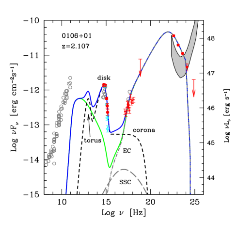
Figure 1: SEDs of 0106+01 (=4C+01.02) together with the fitting models, with parameters listed in Tab. 4. De–absorbed UVOT, XRT and BAT data are indicated by darker symbols (red in the electronic version), while archival data (from NED) are in light grey. Diamonds (and lower arrows, cyan in the electronic version) indicate UVOT data not de–absorbed by intervening Lyman–$\alpha$ clouds. The short–dashed line is the emission from the IR torus, the accretion disk and its X–ray corona. The solid thin (green) line is the non–thermal emission (sum of synchrotron, SSC and EC). The long dashed and the dot–dashed grey lines are the synchrotron self–Compton (SSC) and the External Compton (EC) components, respectively. The thick solid (blue) line is the sum of all components. The grey stripe in the $\gamma$–ray band corresponds to the Fermi/LAT sensitivity of the first 3 months (10$\sigma$, upper boundary) and for 11 months (4$\sigma$, lower boundary).

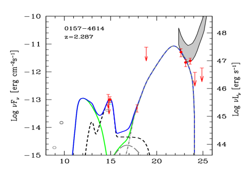
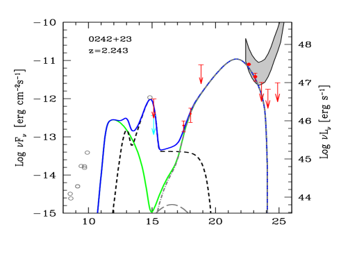
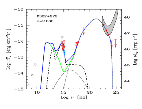
Figure 2: SED of PMN 0157–4614, B2 0242+23 and TXS 0322+222. Symbols and lines as in Fig. 2.

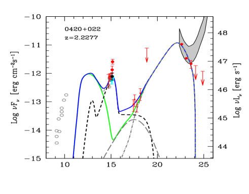
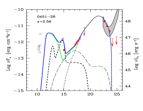
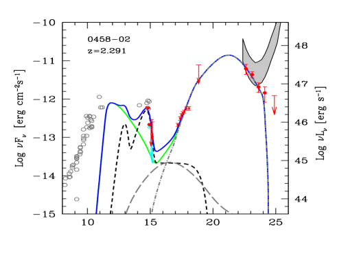
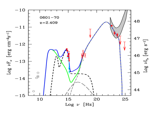
Figure 3: SED of PKS 0420+022, PKS 0451–28, PKS 0458–02 and PKS 0601–70. Symbols and lines as in Fig. 2.

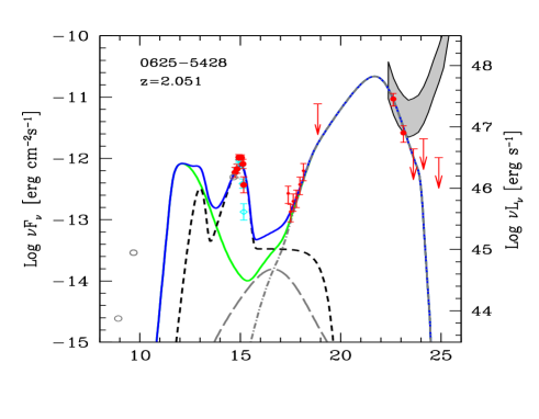
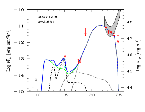
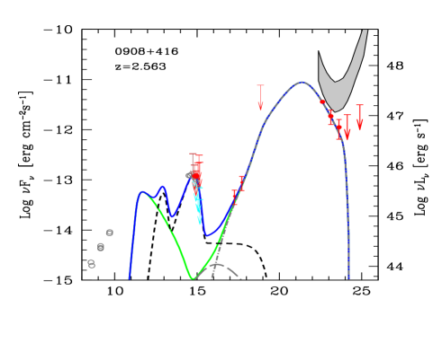
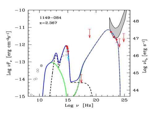
Figure 4: SED of PMN 0625–5438, TXS 0907+230, TXS 0908+416 and PKS 1149–084. Symbols and lines as in Fig. 2.

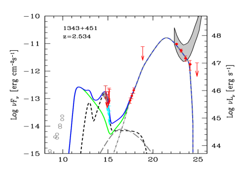
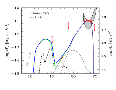
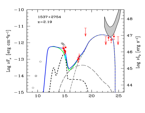
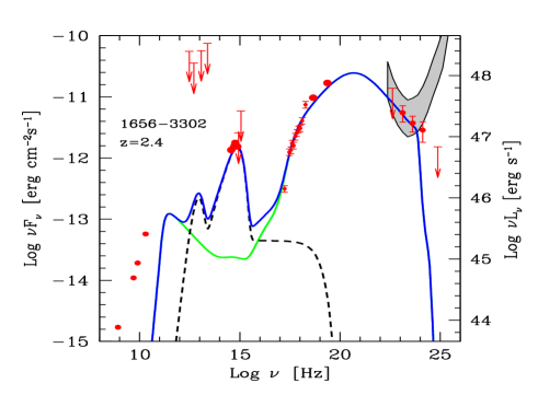
Figure 5: SED of TXS 1343+451, PMN 1344–1723, [WB92] 1537+2754 and SWIFT J1656–3302. Symbols and lines as in Fig. 2.

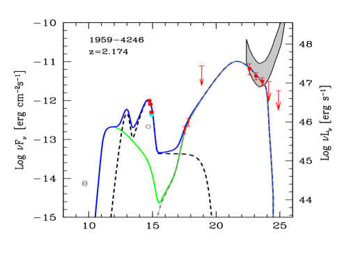
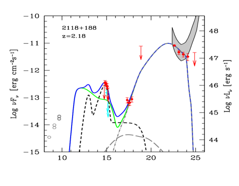
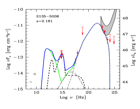
Figure 6: SED of PMN 1959–4246, TXS 2118+188 and PMN 2135–5006 Symbols and lines as in Fig. 2.

4 Modelling the SED

To model the SEDs of the blazars in this sample we used the same model used in G10. It is a one–zone, leptonic model, fully discussed in Ghisellini & Tavecchio (2009). In that paper we emphasize the relative importance of the different sources of the seed photons for the inverse Compton scattering process, and how they change as a function of the distance of the emitting region from the black hole. Here we briefly summarize the main characteristics of the model.

The source is assumed spherical (radius $R$) and located at a distance $R_{\rm diss}$ from the central black hole. The emitting electrons are injected at a rate $Q(\gamma)$ [cm^-3 s^-1] for a finite time equal to the light crossing time $R/c$. The shape of $Q(\gamma)$ we adopt is assumed to be a smoothly broken power law with a break at $\gamma_{\rm b}$:

$$Q(\gamma)\,=\,Q_{0}\,{(\gamma/\gamma_{\rm b})^{-s_{1}}\over 1+(\gamma/\gamma_{\rm b})^{-s_{1}+s_{2}}}$$ (1)

The emitting region is moving with a velocity $\beta c$ corresponding to a bulk Lorentz factor $\Gamma$. We observe the source at the viewing angle $\theta_{\rm v}$ and the Doppler factor is $\delta=1/[\Gamma(1-\beta\cos\theta_{\rm v})]$. The magnetic field $B$ is tangled and uniform throughout the emitting region. We take into account several sources of radiation externally to the jet: i) the broad line photons, assumed to re–emit 10% of the accretion luminosity from a shell–like distribution of clouds located at a distance $R_{\rm BLR}=10^{17}L_{\rm d,45}^{1/2}$ cm; ii) the IR emission from a dusty torus, located at a distance $R_{\rm IR}=2.5\times 10^{18}L_{\rm d,45}^{1/2}$ cm; iii) the direct emission from the accretion disk, including its X–ray corona. Furthermore we take into account the starlight contribution from the inner region of the host galaxy and the cosmic background radiation, but these photon sources are unimportant in our case. All these contributions are evaluated in the blob comoving frame, where we calculate the corresponding inverse Compton radiation from all these components, and then transform into the observer frame.

We calculate the energy distribution $N(\gamma)$ [cm^-3] of the emitting particles at the particular time $R/c$, when the injection process ends. Our numerical code solves the continuity equation which includes injection, radiative cooling and $e^{\pm}$ pair production and reprocessing. Ours is not a time dependent code: we give a “snapshot” of the predicted SED at the time $R/c$, when the particle distribution $N(\gamma)$ and consequently the produced flux are at their maximum.

For all sources in our sample, the radiative cooling time of the particles is short, shorter than $R/c$ even for low energetic particles. In Tab. 4 (last column) we have listed the values of $\gamma_{\rm c}$, that is the minimum value of the random Lorentz factor of electrons cooling in one light crossing time. Since it is always smaller than $\gamma_{\rm b}$, almost all the energy injected in the form of relativistic electrons is radiated away. Most of the cooling is due to the inverse Compton scattering with broad line photons, with a minor contribution from the synchrotron and the self–Compton process. Therefore we always are in the fast cooling regime (i.e. $\gamma_{\rm c}<\gamma_{\rm b}$). In this regime the produced luminosity does not depend on the amount of the radiation energy density, but only on the energy content of the injected relativistic electrons.

Another implication is that, at lower energies, the $N(\gamma)$ distribution is proportional to $\gamma^{-2}$, while, above $\gamma_{\rm b}$, $N(\gamma)\propto\gamma^{-(s_{2}+1)}$. The electrons emitting most of the observed radiation have energies $\gamma_{\rm peak}$ which is close to $\gamma_{\rm b}$ (but these two energies are not exactly equal, due to the curved injected spectrum).

The accretion disk component is calculated assuming a standard optically thick geometrically thin Shakura & Sunjaev (1973) disk. The emission is locally a black body. The temperature profile of the disk is given e.g. in Frank, King & Raine (2002). Since the optical–UV emission is the sum of the accretion disk and the jet non–thermal components, for a few sources there is some degeneracy when deriving the black hole mass and the accretion rate.

We model at the same time the thermal disk (and IR torus) radiation and the non–thermal jet–emission. The link between these two components is given by the amount of radiation energy density (as seen in the comoving frame of the emitting blob) coming directly from the accretion disk or reprocessed by the BLR and the IR torus. This radiation energy density depends mainly on $R_{\rm diss}$, but not on the adopted accretion rate or black hole mass (they are in any case chosen to reproduce the observed thermal disk luminosity).

By estimating the physical parameters of the source we can calculate the power that the jet carries in the form of radiation ($P_{\rm r}$), magnetic field ($P_{\rm B}$), relativistic electrons ($P_{\rm e}$) and cold protons ($P_{\rm p}$) assuming one proton per electron. These powers are calculated according to:

$$P_{\rm i}\,=\,\pi R^{2}\Gamma^{2}cU^{\prime}_{\rm i}$$ (2)

where $U^{\prime}$ is the energy density of the $i_{\rm th}$ component in the comoving frame.

4.1 Intervening Lyman–$\alpha$ absorption

Being at $z>2$ the optical–UV flux of the blazars in our sample could be affected by absorption of neutral hydrogen in intervening Lyman–$\alpha$ absorption systems. To correct for this, we use the attenuation calculated in G10 specifically for the UVOT filters, illustrated in Fig. 3 of that paper.

Full details of our calculation will be described in Haardt et al. (in preparation), together with a more refined treatment of the mean attenuation and its variance around the mean. The current procedure is very crude, especially when the attenuation is large (i.e. optical depths larger than unity) because in such cases most of the attenuation is due to very few clouds, implying a large variance. However, we note that the variance of the attenuation is largely reduced when the actual filter width is taken into account (Madau 1995). Our absorption model results in a mean number of thick systems which is $<1$ for $z\lower 3.22916pt\hbox{$\sim$}\hbox to0.0pt{\hss\raise 1.1625pt\hbox{$<$}}4$, so we do not expect excessive off–set of the attenuation along individual line of sight with respect to the mean value.

When presenting the SED of our sources, we will show both the fluxes and upper limits de–reddened for the extinction due to our Galaxy and the fluxes (and upper limits) obtained by de–absorbing them with the $\tau_{\rm eff}$ shown in Fig. 3 in G10.

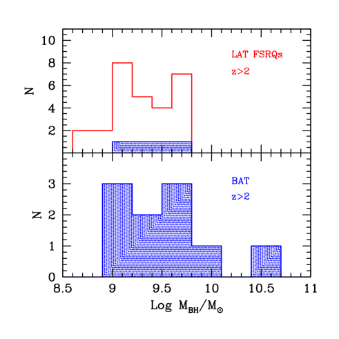
Figure 7: Distribution of the black hole masses derived for the $z>2$ Fermi/LAT (top) and Swift/BAT samples (bottom). The hatched area in the top panel corresponds to the 4 blazars in common.

Name	$z$	$R_{\rm diss}$	$M$	$R_{\rm BLR}$	$P^{\prime}_{\rm i}$	$L_{\rm d}$	$B$	$\Gamma$	$\gamma_{\rm b}$	$\gamma_{\rm max}$	$s_{1}$	$s_{2}$	$\gamma_{\rm c}$
[1]	[2]	[3]	[4]	[5]	[6]	[7]	[8]	[9]	[10]	[11]	[12]	[13]	[14]
0106+01	2.107	900 (600)	5e9	866	0.08	75 (0.1)	1.13	14	300	5e3	0	3.1	2.0
0157–4614	2.287	195 (1.3e3)	5e8	274	0.015	7.5 (0.1)	1.54	15	200	2e3	–1	3.0	5.7
0242+23	2.243	420 (700)	2e9	812	0.022	66 (0.22)	2.13	15	220	2e3	0.5	3.1	2.6
0322+222	2.066	450 (500)	3e9	671	0.06	45 (0.1)	2.06	12	150	3e3	0.5	3.1	3.7
0420+022	2.277	210 (1.4e3)	5e8	725	0.02	52.5 (0.7)	3.79	15	300	2e3	–1	3.2	4.9
0451–28	2.56	540 (450)	4e9	1.1e3	0.24	120 (0.2)	2.66	10	180	2e3	0.	2.6	4.1
0458–02	2.291	472 (450)	3.5e9	606	0.07	37 (0.07)	2.14	10	200	5e3	0.8	3.0	4.9
0601–70	2.409	525 (500)	3.5e9	606	0.05	37 (0.07)	1.83	12.9	190	5e3	–1	3.1	2.8
0625–5438	2.051	270 (900)	1e9	648	0.03	42 (0.28)	2.64	15	240	5e3	0	4.0	3.9
0907+230	2.661	360 (1.5e3)	8e8	290	0.05	8.4 (0.07)	0.36	13	300	1.7e4	0.75	2.8	32.7
0908+416	2.563	180 (600)	1e9	346	0.025	12 (0.08)	1.06	14	150	3e3	0	3.1	7.0
1149–084	2.367	720 (600)	4e9	849	0.015	72 (0.12)	1.39	14	300	3e3	–1	3.0	1.8
1343+451	2.534	420 (700)	2e9	387	0.045	15 (0.05)	1.09	14	150	5e3	–1	2.8	6.5
1344–1723	2.409	330 (1.1e3)	1e9	274	0.027	7.5 (0.05)	0.89	13	1.4e3	8e3	–1	2.5	26.2
1537+2754	2.19	120 (400)	1e9	367	0.015	13.5 (0.09)	4.42	11.5	60	4e3	0.5	2.1	12.2
1656–3302	2.4	525 (700)	2.5e9	1.1e3	0.07	124 (0.33)	1.09	15	70	1e4	0.75	2.85	2.1
1959–4246	2.174	825 (500)	5.5e9	812	0.024	66 (0.08)	1.51	12.9	170	5e3	0	2.7	1.9
2118+188	2.18	270 (600)	1.5e9	424	0.022	18 (0.08)	1.85	14	250	1e4	0.5	2.8	4.6
2135–5006	2.181	189 (900)	7e8	324	0.023	10.5 (0.1)	2.02	14	180	2e3	–1	3.2	6.6
0227–369	2.115	420 (700)	2e9	547	0.08	30 (0.1)	1.5	14	200	5e3	0	3.1	3.0
0347–211	2.944	750 (500)	5e9	866	0.12	75 (0.1)	1.5	12.9	500	3e3	–1	3.0	1.8
0528+134	2.04	420 (1400)	1e9	866	0.13	75 (0.5)	2.6	13	150	3e3	–1	2.8	3.3
0537–286	3.104	420 (700)	2e9	735	0.13	54 (0.18)	1.92	15	50	2e3	–1	3	2.6
0743+259	2.979	1.65e3 (1.1e3)	5e9	866	0.24	75 (0.1)	0.1	15	200	5e3	0.75	2.6	102
0805+614	3.033	270 (600)	1.5e9	581	0.15	34 (0.15)	2.54	14	60	3e3	–0.5	3	4.3
0836+710	2.172	540 (600)	3e9	1.5e3	0.22	225 (0.5)	3.28	14	90	2e3	–1	3.6	2.1
0917–449	2.1899	900 (500)	6e9	1341	0.1	180 (0.2)	1.95	12.9	50	4e3	–1	2.6	1.6
1329–049	2.15	450 (1e3)	1.5e9	822	0.07	67.5 (0.3)	1.4	15	300	5e3	1	3.3	2.5

Table 4: List of parameters used to construct the theoretical SED. Not all of them are “input parameters” for the model, because $R_{\rm BLR}$ is uniquely determined from $L_{\rm d}$, and the cooling energy $\gamma_{\rm c}$ is a derived parameter. Col. [1]: name; Col. [2]: redshift; Col. [3]: dissipation radius in units of $10^{15}$ cm and (in parenthesis) in units of Schwarzschild radii; Col. [4]: black hole mass in solar masses; Col. [5]: size of the BLR in units of $10^{15}$ cm; Col. [6]: power injected in the blob calculated in the comoving frame, in units of $10^{45}$ erg s^-1; Col. [7]: accretion disk luminosity in units of $10^{45}$ erg s^-1 and (in parenthesis) in units of $L_{\rm Edd}$; Col. [8]: magnetic field in Gauss; Col. [9]: bulk Lorentz factor at $R_{\rm diss}$; Col. [10] and [11]: break and maximum random Lorentz factors of the injected electrons; Col. [12] and [13]: slopes of the injected electron distribution [$Q(\gamma)$] below and above $\gamma_{\rm b}$; Col. [14] values of the minimum random Lorentz factor of those electrons cooling in one light crossing time. The total X–ray corona luminosity is assumed to be in the range 10–30 per cent of $L_{\rm d}$. Its spectral shape is assumed to be always $\propto\nu^{-1}\exp(-h\nu/150~{}{\rm keV})$. The viewing angle $\theta_{\rm v}$ is $3^{\circ}$ for all sources.

5 Results

Table 4 lists all parameters used to model the SEDs of our blazars, Table 5 lists the different forms of power carried by the jet and Fig. 1–6 show the SEDs of the 19 blazars studied in this paper and the corresponding fitting model. In all figures we have marked with a grey shaded area the Fermi/LAT sensitivity, bounded on the bottom by considering one year of operation and a 5$\sigma$ detection level, and on the top by considering 3 months and a 10$\sigma$ detection level (this assumes a common energy spectral index of $\alpha_{\gamma}\sim 1$, the sensitivity limit for other spectral indices is slightly different, see Fig. 9 in A10). All these sources were not detected in the first 3 months, in fact the (11 months) $\gamma$–ray data points are very close to the lower boundary of the grey area. There are exceptions: 0106+01 (=4C+01.02) is brighter than the 3–months, 10$\sigma$ sensitivity limits even if it has not been included in LBAS. This is due to a rather strong variability of the source, fainter in the first 3 months and brighter soon after. The same occurred for 1344–1723 and 0451–28. The opposite happened for 0227–369, 0347–211 and 0528+134 (i.e. they were brighter during the first 3 months), but their flux, averaged over 11 months, was in any case large enough to let their inclusion in the 1LAC sample.

Some of the sources have a sufficiently good IR–optical–UV coverage to allow to see a peak of the SED in this band (see for instance 0420+022; 0451–28; 0458–02; 0625–5428; 0907+230; 0908+416; 1149–084; 1656–3302). The other sources have a SED consistent with a peak in this band, but the lack of data also allows for a peak at lower frequencies. We interpret the peak in the optical band as due to the accretion disk, and assume its presence also in those blazars where it is allowed, but not strictly required. By assuming a standard Shakura–Sunyaev (1973) disk we are then able to estimate both the black hole mass and the accretion rate. This important point has been discussed in G10, in Ghisellini et al. (2009) (for S5 0014+813) and in Ghisellini & Tavecchio (2009).

The radio data cannot be fitted by a simple one–zone model specialized to fit the bulk of the emission, since the latter must be emitted in a compact region, whose radio flux is self–absorbed up to hundreds of GHz. The radio emission should come from larger regions of the jet. On the other hand, when possible, we try to have some “continuity” between the non–thermal model continuum and the radio fluxes (i.e. the model, in its low frequency part, should not lie at too low or too high fluxes with respect to the radio data). In the following we briefly comment on the obtained parameters.

Dissipation region — The distance $R_{\rm diss}$ at which most of the dissipation takes place is one of the key parameters for the shape of the overall SED, since it controls the amount of energy densities as seen in the comoving frame (see Ghisellini & Tavecchio 2009). For almost all sources we have $R_{\rm diss}<R_{\rm BLR}$, while for 0106+01, 0907+230, 1343+451, 1344–1723, 1959–4246, $R_{\rm diss}$ is slightly larger than $R_{\rm BLR}$, and for 0743+259 $R_{\rm diss}\sim 2R_{\rm BLR}$.

In all sources the dominant cooling is trough inverse Compton off the seed photons of the BLR. This is true also for the few blazars in which $R_{\rm diss}\geq R_{\rm BLR}$ since, even if $U^{\prime}_{\rm BLR}$ seen in the comoving frame is smaller, also $U_{\rm B}$ is smaller, implying that the ratio $U^{\prime}_{\rm BLR}/U_{B}$ is similar to the values in other sources [$U^{\prime}_{\rm BLR}/U_{B}$ ranges between $\sim$30 (1344–1723) and $\sim$100 (0106+01, 0907+230)]. However, the decreased cooling rate in 0743+259 makes $\gamma_{\rm c}$ to be larger ($\gamma_{\rm c}=102$, see Tab. 4).

With larger still $R_{\rm diss}\gg R_{\rm BLR}$, the main seed photons for the Compton scattering process would became the photons produced by the the IR torus (if it exists), but this case does not occur for our sources.

Compton dominance — This is the ratio between the luminosity emitted at high frequencies and the synchrotron luminosity. The average magnetic field is found to be of the order of 1 Gauss, with a corresponding magnetic energy density that is around two orders of magnitude lower than the radiation energy density. Correspondingly, all sources are Compton dominated.

Black hole masses — Fig. 7 shows the distribution of black hole masses for the 28 blazars at $z>2$ and compares them with the distribution of masses for the high redshift BAT blazars. Although the black hole masses of the BAT sample extend to larger values, there are still too few sources to estimate if the two distributions are different. It is interesting to note that all but 3 sources (0420+022, 0907+230 and 2135–5006) have black hole masses greater than $10^{9}M_{\odot}$. In Ghisellini, Tavecchio & Ghirlanda (2009) we considered the Fermi blazars of $\gamma$–ray luminosity $L_{\gamma}>10^{48}$ erg s^-1, finding, with the same method and model applied here, that for all these sources the black hole mass was greater than a billion solar masses. Therefore all blazars with $L_{\gamma}>10^{48}$ erg s^-1 have black holes heavier than $10^{9}M_{\odot}$, while the vast majority, but not all, blazars at $z>2$ have such large black hole masses. We searched in the literature other estimates of the black hole masses for the objects in this sample, finding $M=2.3\times 10^{9}M_{\odot}$ for 0836+710 (estimated by Liu, Jiang & Gu 2006), and other few limits for the black hole masses for 0836+710 and 0528+134, that were however based assuming an isotropic $\gamma$–ray emission.

Name	$\log P_{\rm r}$	$\log P_{\rm B}$	$\log P_{\rm e}$	$\log P_{\rm p}$
0106+01	46.19	45.88	44.71	47.15
0157–4614	45.51	44.88	44.50	46.71
0242+23	45.68	45.83	44.49	46.96
0322+222	45.91	45.67	44.94	47.36
0420+022	45.64	45.73	44.43	46.68
0451–28	46.35	45.89	45.22	47.53
0458–02	45.81	45.58	44.92	47.32
0601–70	45.91	45.76	44.60	47.00
0625–5438	45.81	45.63	44.73	47.03
0907+230	45.86	44.03	45.30	47.14
0908+416	45.66	44.43	44.80	46.96
1149–084	45.47	45.87	43.83	46.24
1343+451	45.93	45.18	44.94	47.17
1344–1723	45.66	44.74	44.43	46.03
1537+2754	45.24	45.14	44.47	46.58
1656.3–3302	46.17	45.44	45.23	47.88
1959–4246	45.60	46.06	44.19	46.67
2118+188	45.62	45.26	44.50	46.81
2135–5006	45.63	45.03	44.68	46.93
0227–369	46.18	45.49	44.97	47.34
0347–211	46.30	45.91	44.55	46.92
0528+134	47.39	45.86	45.87	48.31
0537-286	46.43	45.74	45.52	48.01
0743+259	46.53	44.36	46.28	47.85
0805+6144	46.42	45.34	45.64	47.99
0836+710	46.60	46.36	45.54	48.00
0917+449	46.20	46.29	45.00	47.57
1329-049	46.18	45.53	45.07	47.65

Table 5: Logarithm of the jet power in the form of radiation ($P_{\rm r}$), Poynting flux ($P_{\rm B}$), bulk motion of electrons ($P_{\rm e}$) and protons ($P_{\rm p}$, assuming one proton per emitting electron). Powers are in erg s^-1. The bottom part of the table reports the data derived in G10 and G09.

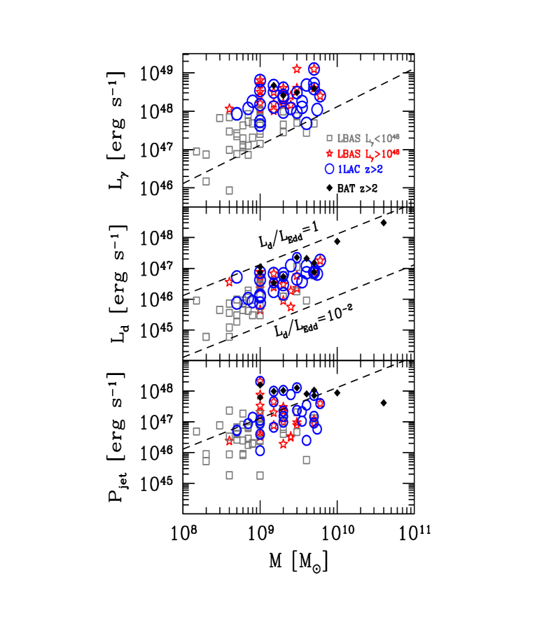
Figure 8: The observed $\gamma$–ray luminosity in the 0.1–10 GeV band, the accretion luminosity $L_{\rm d}$ and the total jet power $P_{\rm jet}$ as a function of the derived black hole mass. All points correspond to FSRQs. Different symbols correspond to LBAS FSRQs with $L_{\gamma}>10^{48}$ erg s^-1 (red stars, analysed in Ghisellini, Tavecchio & Ghirlanda 2009); 1LAC FSRQs with $z>2$ (empty blue circles); BAT FSRQs with $z>2$ (black diamonds, G10) and the LBAS FSRQs with $L_{\gamma}<10^{48}$ erg s^-1 (grey squares, Ghisellini et al. 2010b). The $\gamma$–ray luminosity (top panel) is the observed beamed one, and it has not to be confused with $P_{\rm r}$, the power spent by the jet to produce the radiation we see. The mid panel shows that all FSRQs have disk luminosities between 0.01 and 1 Eddington luminosity. The bottom panel shows that $P_{\rm jet}$ can be larger (but not by a big factor) than the Eddington luminosity corresponding to the dashed line.

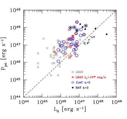
Figure 9: Top: the observed $\gamma$–ray luminosity $L_{\gamma}$ as a function of the accretion luminosity $L_{\rm d}$ for the LBAS FSRQs (grey squares), the $z>2$ 1LAC (blue circles) and Swift/BAT (diamonds) FSRQs. The dashed line indicates $L_{\gamma}=L_{\rm d}$. Mid: the power $P_{\rm r}$ as a function of $L_{\rm d}$. $P_{\rm r}$ can be considered as a robust and almost model–independent lower limit to the jet power. Bottom: the total jet power $P_{\rm jet}=P_{\rm B}+P_{\rm e}+P_{\rm p}$ as a function of $L_{\rm d}$. Almost all sources have $P_{\rm jet}>L_{\rm d}$. One cold proton per emitting electron is assumed.

Disk luminosities — We are considering very powerful blazars, so we do expect large disk luminosities, not only on the basis of an expected positive trend between the observed non–thermal (albeit beamed) and the accretion luminosities, but also on the basis of the observed luminosities of the broad lines, that should linearly depend on the accretion power. What is interesting is that all the FSRQs analyzed up to now (i.e. belonging to the LBAS sample or to the subset of high redshift 1LAC and BAT samples) have a ratio $L_{\rm d}/L_{\rm Edd}$ between 10^-2 and 1. This can be seen in the mid panel of Fig. 8, that shows $L_{\rm d}$ as a function of the derived black hole mass. The two dashed lines correspond to the Eddington and 1% Eddington luminosities. This confirms the idea of the “blazars’ divide” as a result of the changing of the accretion mode (Ghisellini, Maraschi & Tavecchio 2009): from the standard Shakura–Sunyaev (appropriate for all FSRQs) to the ADAF–like regime (appropriate for BL Lacs). The $z>2$ blazars analysed here have $L_{\rm d}/L_{\rm Edd}$ ratios ranging from 0.05 and 0.7. The exact values of the disk luminosities derived here are the frequency integrated bolometric luminosities of the assumed Shakura–Sunyaev accretion disk model that best interpolates the data. On the other hand, any other accretion disk model has to fit the data as well, implying that our values of $L_{\rm d}$ are robust, and nearly model–independent, within the limit of the uncertainties of the observed data.

Jet powers — The values listed in Tab. 5 are very similar to the values derived for other powerful Fermi FSRQs. They are not, however, the absolutely greatest powers found. This can be seen in the bottom panel of Fig. 8, showing $P_{\rm jet}$ as a function of the black hole mass, and in the mid and bottom panels of Fig. 9, where we plot the power of the jet spent in the form of radiation ($P_{\rm r}$) and the total jet power $P_{\rm jet}$ as a function of $L_{\rm d}$. We can compare the $z>2$ 1LAC FSRQs with those present in the LBAS catalogue and the high redshift BAT blazars. Not surprisingly, we see that in these planes the 1LAC $z>2$ sources follow the distribution of the most luminous $\gamma$–ray blazars. Remarkably though, the $z>2$ BAT FSRQs appear to lie at the extreme of the distributions, being the more powerful in $L_{\rm d}$, and among the most powerful in $P_{\rm r}$ and $P_{\rm jet}$. For calculating the power carried by the jet in the form of protons, we re–iterate that we have assumed one cold proton per emitting electron: if there exist a population of cold electrons, and no electron–positron pairs, than we underestimate $P_{\rm p}$ and then $P_{\rm jet}$, while if there are no cold leptons but there are pairs then we overestimate $P_{\rm p}$. Finally, protons are assumed cold for simplicity (and “economy”), but they could be hot or even relativistic (if, e.g. shocks accelerate not only electrons but also protons), and in such cases the power is underestimated. For a detailed discussion about the presence of electron–positron pairs in blazars’ jets we refer to the discussions in Sikora & Madejski (2000), Celotti & Ghisellini (2008) and G10, where one can finds arguments limiting the amount of pairs in the jet. A few electrons–positrons per proton are possible, but not more.

Jet powers vs accretion luminosities — Fig. 9 shows that the correlations found in G10 between $P_{\rm r}$ and/or $P_{\rm jet}$ and $L_{\rm d}$ are confirmed. We remind the reader that $P_{\rm r}$ and $L_{\rm d}$ are independent quantities even if the main radiation mechanism is the inverse Compton process using broad line photons as seeds, that in turn are proportional to the accretion disk luminosity. This is because the radiative cooling of the emitting electrons is complete, implying that the produced jet luminosity becomes independent on the amount of radiation energy density. In other words: in the fast cooling regime the jet always emits all the energy of its relativistic electrons, no matter the amount of the luminosity of the accretion disk.

A least square fit returns a chance probability $P=4\times 10^{-8}$ that $\log P_{\rm r}$ and $\log P_{\rm jet}$ are correlated with $\log L_{\rm d}$ (and the correlation are consistent with being linear). They remain significant also when considering the common redshift dependence, although the chance probability increases to $P=4\times 10^{-4}$ (for the $P_{\rm r}$–$L_{\rm d}$ correlation) and to $P=10^{-3}$ ($P_{\rm jet}$–$L_{\rm d}$).

As expected, the 1LAC blazars at high redshifts are among the most powerful, even if there are blazars at lower redshifts with comparable powers. This can be seen comparing the empty circles, corresponding to the 1LAC blazars of our sample, with the LBAS FSRQs of $L_{\gamma}>10^{48}$ erg s^-1 (stars) and the BAT FSRQs at $z>2$ (black diamonds). There are a few sources with $P_{\rm r}>L_{\rm d}$, and several with $P_{\rm r}\sim L_{\rm d}$. The jet in these blazars, only to produce the radiation we see, requires a power comparable to (or even larger than) the disk luminosity. The $P_{\rm r}$ power should be considered a very robust estimate of the minimum jet power: it is robust because it is almost model–independent ($P_{\rm r}\sim L_{\gamma}/\Gamma^{2}$, see G10), and it is a lower limit because it corresponds to the entire jet power being converted into radiation at the $\gamma$–ray emitting zone. Indeed, if there is one proton per emitting electron, the total jet power, dominated by the bulk motion of cold protons, becomes a factor $\sim 10$ larger than $L_{\rm d}$ (bottom panel of Fig. 9), with the FSRQs of our sample distributed in a large portion of the $P_{\rm jet}$–$L_{\rm d}$ plane.

We believe that the relation between both $P_{\rm r}$ and $P_{\rm jet}$ with $L_{\rm d}$ is a key ingredient to understand the birth of jets: accretion must play a key role.

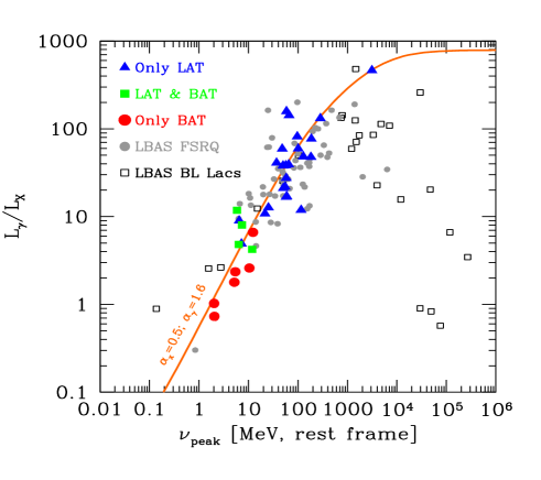
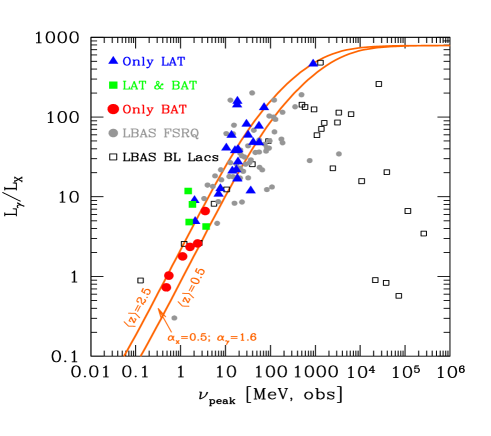
Figure 10: Top: The ratio of the (rest frame) luminosities in the 0.1–100 GeV and 15–55 keV bands as a function of the rest frame peak frequency of the high energy bump. For sources not detected in one of the two bands, we have used the corresponding flux resulting from the modelling of their overall SED. Different symbols are from the sources detected only by Fermi/LAT, by both Swift/BAT and Fermi/LAT and only by Swift/BAT, as labelled. For comparison we also show all FSRQs (grey dots) and BL Lacs (squares) in the LBAS sample. The continuous line shows the estimate using the smoothly broken power law function (see text) with $\alpha_{x}=0.5$ and $\alpha_{\gamma}=1.6$. Bottom panel: the same, but plotting observed peak frequencies. The continuous lines are for $\langle z\rangle=2.5$ and $\langle z\rangle=0.5$. See how the simple function in Eq. 3 interpolates well the data of FSRQs. The X and $\gamma$–ray SED of BL Lacs, instead, is not due to a single radiation process, since the hard X–rays are often due to the tail of the synchrotron emission. As a consequence, they show the opposite behavior of FSRQs: a smaller $L_{X}/L_{\gamma}$ ratio when increasing $\nu_{\rm peak}$, indicating an increasingly stronger contribution of the synchrotron flux to the hard X–ray band.

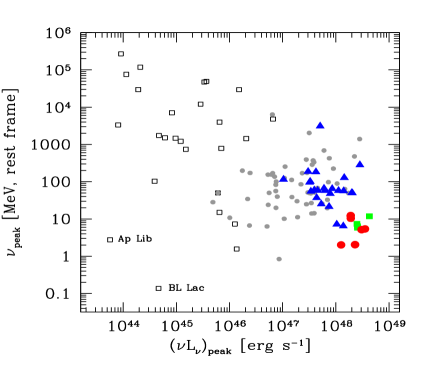
Figure 11: The rest frame peak frequency $\nu_{\rm peak}$ of the high energy emission as a function of the $\nu_{\rm peak}L_{\nu_{\rm peak}}$ luminosity. Symbols as in Fig. 10. A clear trend can be seen when considering BL Lacs and FSRQs together, while FSRQs only are characterized by a very large dispersion. High redshifts FSRQs occupy the region of the largest luminosities and smallest $\nu_{\rm peak}$. We indicate the two “outliers”: BL Lac and Ap Lib.

Comparison with other models — Several groups (Larionov et al. 2008; Marscher et al. 2008, 2010; Sikora, Moderski & Madejski 2008) proposed that the emitting region, especially during flares, is produced at distances from the central black hole of the order of 10–20 pc (much larger than what we assume) at the expected location of a reconfinement shock (e.g. Sokolov, Marscher & McHardy 2004). On the basis of an observed peculiar behaviour of the polarization angle in the optical, Marscher et al. (2008) thus suggested that blobs ejected from the central region are forced by the magnetic field to follow a helical path, accounting for the observed rotation of the polarization angle in the optical. Flares (at all wavelengths) correspond to the passage of these blobs through a standing conical shock, triggered by the compression of the plasma in the shock. This has important consequences for the variability of the emission: since the emission region is located at large distances from the central engine, its size is large, and the expected variability timescale cannot be very short. Assuming $R_{\rm diss}=15$ pc, a jet aperture angle of $\theta_{\rm jet}=3^{\circ}$ and $\delta=20$, we find a minimum variability time scale of $t_{\rm var}=\theta_{\rm jet}R_{\rm diss}(1+z)/(c\delta)$ of the order of 1.5 (1+z) months, that for sources at $z>2$ implies a minimum variability timescales of 5–6 months. The main high energy emission mechanism is still the inverse Compton process, using as seeds the IR radiation of a surrounding torus (Sikora, Moderski & Madejski 2008) with a possible important contribution from jet synchrotron radiation (Marscher et al. 2008, 2010). The main difficulty of these models concerns the expected variability, predicted to occur on a very long time scales, if the size of the emitting region is proportional (through e.g. the opening angle of the jet), to the distance of the source to the black hole. Instead the observed $\gamma$–ray flux in all strong $\gamma$–ray sources (the ones for which a reliable variability behaviour can be established) varies on much shorter time scales, and factor 2 flux changes can occur even on 3–6 hours (see Tavecchio et al. 2010 for 3C 454.3 and PKS 1510–089; Bonnoli et al. 2010; Foschini et al. 2010 and Ackermann et al. 2010 for 3C 454.3; Abdo et al. 2009b for PKS 1454–354; Abdo et al. 2010c for PKS 1502+105). This indicates that the source is compact. This in turn suggests (although it does not prove) that its location cannot be too far from the black hole. It then also suggests that it is within the broad line region. In turn, this suggests that the broad lines are the main seeds for the inverse Compton scattering process. Occasionally, though, dissipation could occur further out, where the main seeds are the infrared photons produced by a putative torus surrounding the accretion disks. Since the seed photons have smaller frequencies, in these cases the produced high energy spectrum suffers less from possible effects of the decreasing (with seed frequencies) scattering Klein–Nishina cross section and less from possible photon–photon interactions leading to electron–positron pair production. The decreased importance of both effects may account for high energy spectra extending, unbroken, up to hundreds of GeV. These cases should be characterized by a longer variability timescale.

In the model of Marscher et al. (2008) a very short variability timescale still indicates a very compact emitting region, but nevertheless located at a large distance from the central black hole.

5.1 Comparing BAT and LAT high redshift blazars

Both the 1LAC sample and the BAT 3–years survey have a rather uniform sky coverage, and both approximate a flux limited sample. The 1LAC sample has a limiting flux sensitivity that depends on the $\gamma$–ray spectral index of the sources, but since we are dealing with FSRQs only (whose $\alpha_{\gamma}$ is contained in a relatively narrow range), we can consider this sample as flux limited. It is then interesting to compare the high redshift blazars (all of them are FSRQs) contained in the two samples. We remind that for blazars with $z>2$, we have 10 FSRQs in the BAT sample, 28 in the 1LAC, and 4 in both. The X–ray to $\gamma$–ray SED of these sources is very similar: even if we have only 4 blazars in common, for all sources the SED has a high energy peak in the $\sim$MeV–100 MeV band, with $\alpha_{x}<1$ and $\alpha_{\gamma}>1$.

Thus the spectrum can be approximated by a broken power law. For illustration, consider the smoothly broken power law of the form

$$L(\nu)\propto{(\nu/\nu_{\rm b})^{-\alpha_{x}}\over 1+(\nu/\nu_{\rm b})^{\alpha_{\gamma}-\alpha_{x}}}$$ (3)

If the energy indices $\alpha_{x}<1$ and $\alpha_{\gamma}>1$, the peak is at $\nu_{\rm peak}=\nu_{\rm b}[(1-\alpha_{x})/(\alpha_{\gamma}-1)]^{1/(\alpha_{\gamma}-\alpha_{x})}$. With this function we can easily calculate the ratio of the BAT [15–55 keV] to LAT [0.1–100 GeV] luminosities as a function of $\nu_{\rm peak}$, and see if it compares well to the data. We alert the reader that by “data” we mean real observed data when the source has been detected in the X–ray and $\gamma$–ray band, while, when the detection is missing, we mean the “data” coming from our fitting model described in §4 (and in more detailed in Ghisellini & Tavecchio 2009).

The ratio $L_{X}/L_{\gamma}$ as a function of $\nu_{\rm peak}$ calculated using Eq. 3 setting $\alpha_{x}=0.5$ and $\alpha_{\gamma}=1.6$ is plotted in Fig. 10 as a grey (orange in the electronic version) line, together with the points corresponding to high redshift blazars, studied in this paper and in G10. Furthermore, Fig. 10 reports also the data of all the LBAS blazars studied in Ghisellini et al. (2010b). These are FSRQs (filled grey circles) and BL Lacs (empty grey squares). In the top panel $\nu_{\rm peak}$ is in the rest frame of the source, while in the bottom panel $\nu_{\rm peak}$ is the observed one.

Fig. 10 shows a remarkable agreement between the FSRQ data and the simple broken power law of Eq. 3, both for high redshifts and for less distant FSRQs. BL Lac objects, instead, are not well represented by Eq. 3. In fact, in many BL Lacs the hard X–rays correspond to the (steep) tail of the synchrotron component. Therefore the X and the $\gamma$–rays are produced by two different mechanisms, and Eq. 3 does not represent their overall high energy SED. In BL Lacs the importance of X–rays increases increasing $\nu_{\rm peak}$, because of the increasing importance of synchrotron flux in the hard X–rays.

Coming back to high redshift FSRQs, only 4 sources have detection in both bands, while 24 FSRQs are detected only by the LAT and 6 only by the BAT instrument. Our model explains the large fraction of sources that are detected only in one of the two instruments as due to the different $\nu_{\rm peak}$ of the sources: if $\nu_{\rm peak}$ is large (above 10 MeV), $F_{\gamma}/F_{X}$ is large and the source is relatively weak in the BAT band, while if $\nu_{\rm peak}<$10 MeV the source becomes relatively weak in the LAT band and strong in the BAT.

It is interesting to see if the derived $\nu_{\rm peak}$ correlates with the bolometric luminosity. Fig. 11 shows that a trend indeed exists: more powerful sources have smaller $\nu_{\rm peak}$ (we have used $\nu_{\rm peak}L_{\nu_{\rm peak}}$ as a proxy for the bolometric luminosity). But comparing with all the LBAS FSRQs (grey dots) we see that the $z>2$ luminous FSRQs belong to a broader (i.e. more scattered) distribution, and that the high–$z$ BAT blazars are really the most extreme.

We can conclude that i) there is a a trend between the high energy peak and the peak luminosity, ii) that this correlation has a large scatter, even if iii) the $z>2$ FSRQs show the same trend with less scatter (but this may be due to the still small number) and finally iv) the $z>2$ blazars in the 3–years BAT survey all lie in the highest luminosity, smallest $\nu_{\rm peak}$ part of the plane.

When more BAT detections of high redshift LAT blazars will become available (and, conversely, when LAT will detect more BAT high–$z$ blazars) this trend can be tested directly (i.e. without modelling the SED). The importance of this is two–fold: first we can estimate in a reasonable way the peak energy of the high energy emission having the hard X–ray and the $\gamma$–ray luminosities, and second (and more important) we could conclude that the most powerful blazars can be more easily picked up trough hard X–ray surveys, as the one foreseen with the EXIST mission (Grindlay et al. 2010).

6 Summary and discussion

The total number of $z>2$ blazars with high energy information is 34 (28 with a LAT detection, 6 with BAT, and 4 with both). It is still a limited number, the tip of the iceberg of a much larger (and fainter) population, but it is derived from two well defined samples (LAT and BAT), that we can consider as flux limited and coming from two all sky surveys (excluding the galactic plane). The main result of studying them is that all the earlier findings concerning the physical parameters of the jet emitting zone, the jet power, and the correlation between the jet power and the disk luminosity are confirmed.

They are in agreement with the blazar sequence, i.e. their non–thermal SED are “redder” than less luminous blazar, with a large dominance of their high energy emission over the synchrotron one. This implies that the disk emission is left unhidden by the synchrotron flux, and this allows an estimate of the black hole mass and the accretion rate. The uncertainties associated with these estimates are relatively small within the assumption that the thermal component is produced by a standard Shakura–Sunyaev disk with an associated non–spinning hole. In G10 we argued that in any case the masses are not largely affected by this assumption, and in particular that in the Kerr case the derived masses are not smaller, despite the greater accretion efficiency. The possibility of an intrinsic collimation of the disk radiation appears more serious. If the disk is not geometrically thin, but e.g. a flared disk, then we expect a disk emission pattern concentrated along the normal to the disk, i.e. along the jet axis. We argued previously (Ghisellini et al. 2009) that this can be the case of S5 0014+813 at $z=3.366$, an extraordinary luminous blazars (detected by BAT) with an estimated “outrageous” black hole mass of $4\times 10^{10}M_{\odot}$. And indeed we found it to be an “outlier” in the $P_{\rm r}$–$L_{\rm d}$ plane. Reverting the argument, it implies that the other FSQRs, obeying a well defined $P_{\rm r}$–$L_{\rm d}$ trend, should have disk luminosities with a quasi–isotropic pattern, i.e. standard, not flaring, disks. The other severe uncertainty on the mass estimation for objects at large redshifts is the amount of attenuation of their optical–UV flux, due to intervening Lyman–$\alpha$ clouds. We have corrected for this assuming an average distribution of clouds, and when the attenuation is due to a few thick clouds the expected variance is large. While we plan to refine such estimates (Haardt et al. in preparation), it is unlikely that this implies a systematic error on the mass estimates, leading to larger values: statistically, the mass distribution should not be seriously affected by this uncertainty.

Although affected by the same issues outlined above, also the correlation between the jet power and the disk luminosity should resist when a more refined treatment of the Lyman–$\alpha$ absorption will be available, by the same arguments. Therefore we can conclude that the accretion rate is really a fundamental player in powering the relativistic jet, and we refer the reader to Ghisellini et al. (2010b) for a detailed discussion about this finding. If true, these ideas lead us to suggest that powerful, high redshifts “true” (i.e. really lineless) BL Lacs do not exist.

Another, at first sight surprising, result of our study is that the correlation between the peak frequency of the high energy emission and the $\gamma$–ray luminosity at this peak frequency exists also for the $z>2$, highly luminous FSRQs. It is surprising because in very powerful sources the radiative cooling is complete (i.e. all electrons with $\gamma$ larger than an few cool in one light crossing time). Therefore the electrons responsible for the peak have energies that are not fixed by radiative cooling, but by the injection function [i.e. by the $Q(\gamma)$ function given in Eq. 1, and more precisely by the value of $\gamma_{\rm b}$]. On the other hand, when considering all blazars in the LBAS sample, we see that the scatter, for large luminosities, is much larger, so the apparent correlation for the $z>2$ blazars can be due to small statistics. Clearly, it is a point to investigate further.

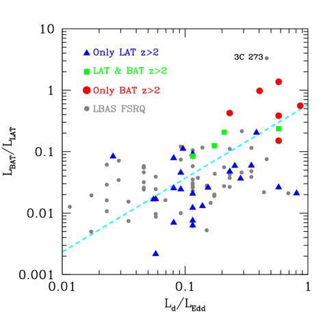
Figure 12: The ratio between the luminosities in the BAT and LAT energy ranges (i.e. 15–55 keV and 0.1–10 GeV) as a function of the disk luminosity, in Eddington units. Big dots are the 6 BAT blazars in the $z>2$ sample not detected (yet) by Fermi/LAT, squares are BAT blazars of the same sample already present in the 1LAC sample, triangles are the sources discussed in this paper, and the small grey dots are all the FSRQs present in the LBAS sample discussed in G10. The dashed line is the best least square fit (chance probability $P=2\times 10^{-6}$).

It is interesting to ask what will be the best strategy to find the most luminous FSRQs at the largest redshifts. The interest lies in the link between jet power and disk luminosity: finding the most powerful jets implies to find the most accreting systems, hence the heaviest black holes. Since for each source pointing at Earth (i.e. a blazar) there must exist $\sim 2\Gamma^{2}$ similar sources pointing in other directions, the finding of even a few blazars at large redshifts with a large black hole mass can put very interesting constraints on the black hole mass function of jetted sources. This issue has been discussed by us previously (G10), and we suggested that the existence of the blazar sequence, plus an important K–correction effect, makes the hard X–ray range the best band where to search for the high–$z$ heaviest black holes. Here we re–iterate this suggestion offering a supplementary information. For each analyzed FSRQs (belonging to the LBAS sample, or in this paper), we have calculated the ratio between the expected BAT luminosity [15–55 keV, rest frame] and the observed [0.1–100 GeV, rest frame] LAT luminosity. This ratio is not an observed quantity, since very few FSRQs (in comparison with LAT) have been detected by BAT, but it is a result of the model. Then, with the same model, we have calculated the disk luminosity in units of Eddington. Fig. 12 shows the $L_{\rm BAT}/L_{\rm LAT}$ ratio as a function of $L_{\rm d}/L_{\rm Edd}$. We have marked with different symbols the FSRQs analyzed in this paper and the ones analysed previously (G10). We have excluded BL Lacs for which we have only an upper limit on the disk luminosity. Fig. 12 suggests a clear trend (albeit with some scatter): FSRQs accreting close to Eddington emit relatively more in the hard X–rays than above 100 MeV. Formally, a least square fit returns $(L_{\rm BAT}/L_{\rm BAT})\propto(L_{\rm d}/L_{\rm Edd})^{1.2}$ with a chance probability $P=2.\times 10^{-6}$ (for 95 objects). This implies that hard X–ray surveys benefit of a positive bias when looking for blazars with black holes accreting close to Eddington. In turn, at high–$z$, this implies the finding of the heaviest black holes, since it is very likely that at those early epochs (e.g. $z>2$) all black holes are accreting close to the Eddington rate.

7 Conclusions

We summarize here our main conclusions:

• The blazars detected by Fermi at $z>2$ are all FSRQs, with typical “red” SEDs.

• These FSRQs are very luminous and powerful, but they are not at the very extreme of the distribution of luminosity and jet power.

• These sources have heavy black holes ($M\sim 10^{9}M_{\odot}$) and accretion luminosities greater than $\sim$10% Eddington. When including all FSRQs in the LBAS sample, irrespective of redshift, the accretion disk luminosities is greater than 1% Eddington.

• The trend of redder SED when more luminous (i.e. one of the defining characteristics of the blazar sequence) is confirmed, and it is even present within the relatively small range of observed luminosity of the $z>2$ blazars.

• The correlation between the jet power and the disk luminosity is confirmed and points to a crucial role played by accretion in powering the jet.

• FSRQs with accretion disks closer to the Eddington luminosity have jets emitting a “redder” SED, and therefore can be more efficiently picked up by hard X–ray surveys (such as the one foreseen by EXIST), rather than by surveys in the hard $\gamma$–ray band.

References

- [] Abdo A.A., Ackermann M., Ajello M. et al., 2009a , ApJ, 700, 597 (A09)
- [] Abdo A.A., Ackermann M., Ajello M. et al., 2009b, ApJ, 697, 934
- [] Abdo A.A., Ackermann M., Ajello M. et al., 2010a, ApJS, 188, 405
- [] Abdo A.A., Ackermann M., Ajello M. et al., 2010b, ApJ, 715, 429 (A10)
- [] Abdo A.A., Ackermann M., Ajello M. et al., 2010c, ApJ, 710, 810
- [] Ackermann M., Ajello M., Baldini L. et al., 2010, subm to ApJ (astro–ph/1007.0483)
- [] Ajello M., Costamante L., Sambruna R.M., et al., 2009, ApJ, 699, 603
- [] Bonnoli G., Ghisellini G., Foschini L., Tavecchio F., Ghirlanda G., 2010, MNRAS, in press (astro–ph/1003.3476)
- [] Cardelli J.A., Clayton G.C. & Mathis J.S., 1989, ApJ, 345, 245
- [] Cash W., 1979, ApJ, 228, 939
- [] Celotti A. & Ghisellini G., 2008, MNRAS, 385, 283
- [] Donato D., Ghisellini G., Tagliaferri G. & Fossati G., 2001, A&A, 375, 739
- [] Foschini L., Tagliaferri G., Ghisellini G., Ghirlanda G., Tavecchio F. & Bonnoli G., 2010, MNRAS, in press (astro–ph/1004.4518)
- [] Fossati G., Maraschi L., Celotti A., Comastri A. & Ghisellini G., 1998, MNRAS, 299, 433
- [] Frank J., King A. & Raine D.J., 2002, Accretion power in astrophysics, Cambridge (UK) (Cambridge University Press)
- [] Ghirlanda G., Ghisellini G., Tavecchio F., Foschini L. 2010, MNRAS, in press (astro–ph/1003.5163)
- [] Ghisellini G., Celotti A., Fossati G., Maraschi L. & Comastri A., 1998, MNRAS, 301, 451
- [] Ghisellini G. & Tavecchio F., 2009, 397, 985 MNRAS
- [] Ghisellini G., Tavecchio F. & Ghirlanda G., 2009, MNRAS 399, 2041
- [] Ghisellini G., Foschini L., Volonteri M., Ghirlanda G., Haardt F., Burlon D., Tavecchio F., 2009, MNRAS, 399, L24
- [] Ghisellini G., Maraschi L. & Tavecchio F., 2009, MNRAS, 396, L105
- [] Ghisellini G., Della Ceca R., Volonteri M. et al., 2010a, MNRAS, 405, 387 (G10)
- [] Ghisellini G., Tavecchio F., Foschini L., Ghirlanda G., Maraschi L., Celotti A., 2010b, MNRAS, 402, 497
- [] Grindlay J., Bloom J., Coppi P. et al., 2010, in X–ray Astronomy 2009: Present status, multiwavelength approach and future perspectives”, to appear in AIP Conf. Proc. (editors: A. Comastri, M. Cappi, L. Angelini) (astro–ph/1002.4823)
- [] Kalberla P.M.W., Burton W.B., Hartmann D., Arnal E.M., Bajaja E., Morras R. & Pöppel W.G.L., 2005, A&A, 440, 775
- [] Larionov V.M. et al., 2008, A&A 492, 389
- [] Liu Y., Jiang D.R. & Gu M.F., 2006, ApJ, 637, 669
- [] Madau P., 1995, ApJ, 441, 18
- [] Marscher A.P., et al. 2008, Nat., 452, 966
- [] Marscher A.P., et al. 2010, ApJ, 461, L126
- [] Poole T.S., Breeveld A.A., Page M.J. et al., 2008, MNRAS, 383, 627
- [] Roming P.W.A., Kennedy T.E., Mason K.O. et al., 2005, Space Sci. Rev., 120, 95
- [] Sikora M., Moderski R. & Madejski G.M., 2008, ApJ, 675, 71
- [] Sikora M. & Madjesi G., 2000, ApJ, 534, 109
- [] Shakura N.I. & Sunyaev R.A., 1973 A&A, 24, 337
- [] Sokolov A., Marscher A.P. & McHardy I.M., 2004, ApJ, 613, 725
- [] Tavecchio F. & Ghisellini G., 2008, MNRAS, 386, 945
- [] Tavecchio F., Ghisellini G., Bonnoli G. & Ghirlanda G., 2010, MNRAS, 405, L94