Comment on “Optical precursors in the singular and weak dispersion limits”

Abstract

We point out inconsistencies in the recent paper by Oughstun et al. on Sommerfeld and Brillouin precursors [J. Opt. Soc. Am. B 27, 1664-1670 (2010)]. Their study is essentially numerical and, for the parameters used in their simulations, the difference between the two limits considered is not as clear-cut as they state. The steep rise of the Brillouin precursor obtained in the singular limit and analyzed as a distinguishing feature of this limit simply results from an unsuitable time scale. In fact, the rise of the precursor is progressive and is perfectly described by a Airy function. In the weak dispersion limit, the equivalence relation, established at great length in Section 3 of the paper, appears as an immediate result in the retarded-time picture. Last but not least, we show that, contrary to the authors claim, the precursors are catastrophically affected by the rise-time of the incident optical field, even when the latter is considerably faster than the medium relaxation time.

OCIS codes: 260.2030, 320.5550, 320.2250.

In a recent paper ou10 , Oughstun et al. revisit the classical problem of the propagation of a step modulated pulse in a Lorentz model medium. They specifically consider the case where the absorption line is narrow (singular limit) and the one where the refractive index of the medium keeps very close to unity at every frequency (weak dispersion limit). The medium is characterized by its complex refractive index

$$n(\omega)=\left(1-\frac{\omega_{p}^{2}}{\omega^{2}-\omega_{0}^{2}+2i\delta\omega}\right)^{1/2}.$$ (1)

Here $\omega$, $\omega_{p}$, $\omega_{0}$ and $\delta$ respectively designate the current optical frequency, the plasma frequency, the resonance frequency and the damping or relaxation rate. The wave propagates in the $z$-direction. In the following we use the retarded time $t$, equal to the real time minus $z/c$ where $c$ is the velocity of light in vacuum (retarded time picture). The medium is then characterized by the transfer function

$$H(\omega)=\exp\left[i\frac{\omega}{c}z\left(n(\omega)-1\right)\right]$$ (2)

and the field transmitted $E(z,t)$ at the abscissa $z$ reads as

$$E(z,t)=\frac{1}{2\pi}\int_{-\infty+ia}^{+\infty+ia}H(\omega)\widetilde{E}(0,\omega)\exp(-i\omega t)\mathrm{d}\omega.$$ (3)

Here $a$ is a positive constant and $\widetilde{E}(0,\omega)$ is the Fourier transform of the incident field $E(0,t)$. In ou10 , the latter is assumed to have the idealized form

$$E(0,t)=\Theta(t)\sin(\omega_{c}t)$$ (4)

where $\Theta(t)$ is the unit step function and $\omega_{c}$ is the frequency of the optical carrier.

Although it abundantly refers to the theoretical results obtained by the asymptotic method, the study reported in ou10 is mainly numerical. All the simulations are made for $\omega_{0}=3.9\times 10^{14}\mathrm{rad/s}$ re1 and $\omega_{c}=3.0\times 10^{14}\mathrm{rad/s}$ in a normal dispersion region. The singular and weak dispersion limits are respectively attained when $\delta\ll\omega_{0}$ and $\omega_{p}^{2}\ll\delta\omega_{0}$ [see Eq. (1)]. Oughstun et al. emphasize that these two limiting cases “are fundamentally different in their effects upon propagation” but, surprisingly enough, they take for their simulations in the weak dispersion limit a value of $\delta$ for which the singular limit nearly holds ($\delta<\omega_{0}/100$). Consequently, mutatis mutandis, the results obtained in the two limits appears qualitatively similar. The steep rise of the Brillouin precursor obtained in the singular limit (their Fig.3) and analyzed as a distinguishing feature of this limit is only due to an unsuitable time scale. As shown in our Fig.1, obtained for the same values of the parameters, the rise is quite progressive and well reproduced by a Airy function.

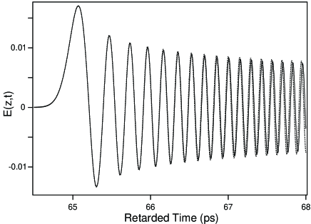
Figure 1: Brillouin precursor obtained for the parameters of the figure 3 of ou10 , that is for $\omega_{0}=3.9\times 10^{14}\mathrm{rad/s}$, $\omega_{c}=3.0\times 10^{14}\mathrm{rad/s}$, $\omega_{p}=3.05\times 10^{14}\mathrm{rad/s}$ , $\delta=3.02\times 10^{10}\mathrm{rad/s}$, and $z=7.232\times 10^{-2}\mathrm{m}$. The full line is the exact numerical solution obtained by fast Fourier transform (FFT) and the dashed line is the approximate analytical solution given by Eq.7.

This result, established by Brillouin himself in 1932 bri32 , is easily retrieved from Eqs (1), (2), and (3). Anticipating that the beginning of the precursor involves frequencies $\omega$ such that $\delta\ll\omega\ll\omega_{c}$, we use the approximate relations

$$n(\omega)\approx\left(1+\frac{\omega_{p}^{2}}{\omega_{0}^{2}}\right)^{1/2}+\frac{\omega^{2}\omega_{p}^{2}}{2\omega_{0}^{3}\left(\omega_{0}^{2}+\omega_{p}^{2}\right)^{1/2}}$$ (5)

and $\widetilde{E}(0,\omega)\approx 1/\omega_{c}$. Introducing the new retarded time $t^{\prime}=t-t_{b}$ with $t_{b}=\frac{z}{c}\left[\left(1+\omega_{p}^{2}/\omega_{0}^{2}\right)^{1/2}-1\right]$, the transfer function then reads as $\exp\left[i\omega^{3}/\left(3b^{3}\right)\right]$ where

$$b=\omega_{0}\left[\frac{2c\left(\omega_{0}^{2}+\omega_{p}^{2}\right)^{1/2}}{3z\omega_{p}^{2}}\right]^{1/3}.$$ (6)

We finally get

$$E(z,t^{\prime})=\frac{1}{2\pi\omega_{c}}\int_{-\infty}^{+\infty}\exp\left(\frac{i\omega^{3}}{3b^{3}}-i\omega t^{\prime}\right)\mathrm{d}\omega=\frac{b}{\omega_{c}}\mathrm{Ai}(-bt^{\prime})$$ (7)

where $\mathrm{Ai}(x)$ is the Airy function re2 . As it appears Fig.1, this analytic expression perfectly fits not only the rise of the precursor but also a significant number of its subsequent oscillations. Equations (6) and (7) also provide a simple evidence of the $z^{-1/3}$ dependence of the precursor amplitude on the propagation distance. Figure 2 shows the Brillouin precursor obtained in the conditions of the Figure 5 of ou10 , intended to illustrate the specific case of the weak dispersion limit. As indicated previously, the conditions of the singular limit are approximately met and this explains why the first oscillation of the precursor and thus its peak amplitude are well reproduced by Eq. (7). Note that the rise-time of the precursor, proportional to $1/b$, is 6 times faster than in the previous case.

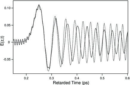
Figure 2: Same as Fig.1 for the parameters of the figure 5 of ou10 , that is for $\omega_{0}=3.9\times 10^{14}\mathrm{rad/s}$, $\omega_{c}=3.0\times 10^{14}\mathrm{rad/s}$, $\omega_{p}=3.05\times 10^{12}\mathrm{rad/s}$ , $\delta=3.02\times 10^{12}\mathrm{rad/s}$, and $z=2.290\mathrm{m}$. The rapid oscillations of small amplitude superposed upon the beginning of the Brillouin precursor are the end of the Sommerfeld precursor.

In their study of the weak dispersion limit, Oughstun et al. ou10 mention a “curious difficulty in the numerical FFT simulation of pulse propagation” and, in order to overcome it, they develop at great length an equivalence relation. In fact the difficulty is completely avoided in the retarded-time picture and their equivalence relation then appears as an immediate result. In the weak dispersion limit, the transfer function, as given by Eq.(2), is indeed reduced to

$$H(\omega)\approx\exp\left[-\frac{i\omega}{2c}\left(\frac{\omega_{p}^{2}z}{\omega^{2}-\omega_{0}^{2}+2i\delta\omega}\right)\right].$$ (8)

This only expression shows that, for given $\omega_{0}$ and $\delta$, all the media having the same $\omega_{p}^{2}z$ (and thus the same optical thickness at any reference frequency) are equivalent.

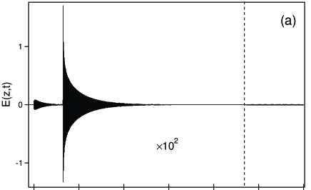
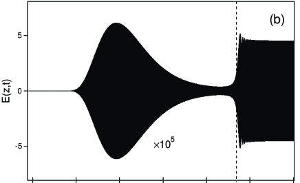
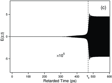
Figure 3: Effect of the rise-time of the incident field on the transmitted field. The parameters are those of the figure 3 of ou10 , that is $\omega_{0}=3.9\times 10^{14}\mathrm{rad/s}$, $\omega_{c}=3.0\times 10^{14}\mathrm{rad/s}$, $\omega_{p}=3.05\times 10^{14}\mathrm{rad/s}$ , $\delta=3.02\times 10^{10}\mathrm{rad/s}$, and $z=7.232\times 10^{-2}\mathrm{m}$. The vertical dashed line indicates the group delay $\tau_{g}=\frac{\mathrm{d}\varphi}{\mathrm{d}\omega}\left|{}_{\omega=\omega_{c}}\right.$ where $\varphi$ is the argument of $H(\omega)$ ($\tau_{g}=471\mathrm{ps}$). $\tau_{g}$ fixes the arrival of the “main field” whose amplitude, equal to $\exp\left(-10\right)\approx 4.5\times 10^{-5}$, obviously does not depend on the rise-time. The different curves are obtained for (a) $T_{r}=0$, (b) $T_{r}=\tau/500$, and (c) $T_{r}=\tau/100$ where $\tau=1/\delta$ is the relaxation or damping time of the medium.

In a real experiment, the incident field is obviously turned on in a finite time. Oughstun et al. state that their “results will remain valid for a non instantaneous turn-on signal provided that the signal turn-on time $T_{r}$ is faster than the characteristic relaxation time $1/\delta$”. This is grossly false. Figure 3 shows the results of a simulation performed for the parameters of their figure 3 and $10-90\%$ turn-on times (a) $T_{r}=0$, (b) $T_{r}=\tau/500$, and (c) $T_{r}=\tau/100$ where $\tau=1/\delta$ is the relaxation or damping time ($\tau\approx 33\mathrm{ps}$). The rise of the incident field is modelled by replacing the step-function $\Theta(t)$ appearing in the idealized form of Eq. (4) by $f(t)=\frac{1}{2}\left[1+\mathrm{erf}(\xi t)\right]$ where $\mathrm{erf}(x)$ designates the error function. The corresponding rise-time is $T_{r}\approx 1.8/\xi$ and $f(t)\rightarrow\Theta(t)$ when $\xi\rightarrow\infty$. We see that the effect of the rise-time is actually catastrophic. For a rise-time as fast as $\tau/500$ ($\approx 66\mathrm{fs}$ ), the Sommerfeld precursor is absent. The maximum of the Brillouin precursor is significantly time-delayed and its amplitude $A_{B}$ is reduced by a factor of about 300, becoming comparable to the amplitude $\mathrm{e}^{-10}$ of the “main field”. The reduction factor obviously depends on the optical thickness and, consequently, the power law $A_{B}\propto z^{-1/3}$, obtained for $T_{r}=0$, breaks down. Finally the curve (c) of Fig.3 shows that both precursors practically vanish for $T_{r}=\tau/100$ . By means of other simulations, we find that the Sommerfeld precursor is very attenuated as soon as $T_{r}>\tau/5000\approx 2/\omega_{c}$ and that a correct reproduction of both precursors as obtained for $T_{r}=0$ requires that $T_{r}\leq 1/\omega_{c}$. This condition results from the fact that the Sommerfeld (Brillouin) precursor mainly involves frequencies $\omega\gg\omega_{c}$ ($\omega\ll\omega_{c}$) and thus is excited by the corresponding frequencies contained in the spectrum of the incident field. From the expression of $f(t)$, it is easily shown that the effect of a finite rise-time $T_{r}$ ($T_{r}\approx 1.8/\xi$ ) is to divide $\widetilde{E}(0,\omega)$ by $\exp\left[\omega^{2}/\left(4\xi^{2}\right)\right]$ when $\omega/\omega_{c}\rightarrow\infty$ and by $\exp\left[\omega_{c}^{2}/\left(4\xi^{2}\right)\right]$ when $\omega/\omega_{c}\rightarrow 0$. These expressions explain why the Sommerfeld precursor is much more affected by the rise-time effects than the Brillouin precursor and enable one to predict that, for $T_{r}=1/\omega_{c}$ ($\xi\approx 1.8\omega_{c}$), the amplitude $A_{B}$ of the Brillouin precursor will be about $7.5\%$ below that obtained for $T_{r}=0$ (result confirmed by an exact numerical calculation).

The observation of a signal close to that shown on the figure 3 of ou10 requires not only that the rise-time of the incident field does not exceed $1/\omega_{c}$ ($3.3\mathrm{fs}$) but also that its subsequent amplitude remains nearly constant during a time that would be more than four orders of magnitude longer. The fulfilment of this double condition, either with a pulsed laser or with a continuous wave laser followed by a modulator, appears to be quite unrealistic from an experimental viewpoint. More generally, due to such temporal constraints, we don’t see how the Brillouin precursor could be actually used in optics as a tool for imaging through a dense medium, opaque at the carrier frequency. Anyway, the problem of optical precursors is of fundamental interest from a theoretical viewpoint, even if the experiment imagined by Sommerfeld and Brillouin may appear as a gedankenexperiment. In this spirit, we are examining what the precursors become when the incident field $E(0,t)=\Theta(t)\sin(\omega_{c}t)$, constantly considered in the theoretical papers, is replaced by $E(0,t)=\Theta(t)\cos(\omega_{c}t)$. The true discontinuity of the incident field at the initial time then leads to radically new effects that we will discuss in a forthcoming paper.

References

- (1) KE Oughstun, N.A. Cartwright, D.J. Gauthier, and H Jeong, “Optical precursor in the singular and weak dispersion limits,” J. Opt. Soc. Am. B 27, 1664-1670 (2010).
- (2) Contrary to what is stated in ou10 , this (circular) frequency is not equal to the frequency of the resonance involved in the experiment on cold potassium atoms but is times smaller.
- (3) L. Brillouin, “Propagation des ondes électromagnétiques dans les milieux matériels,” in Comptes Rendus du Congrès International d’Electricité, Paris 1932 (Gauthier-Villars 1933), Vol.2, pp 739-788. An English adaptation of this paper can be found in L. Brillouin, Wave Propagation and Group Velocity (Academic 1960), Ch. IV and Ch. V.
- (4) Note that the Airy function used by Brillouin in bri32 differs from the standard one used in the present comment, with . Peak amplitudes of and are respectively 2.33 and 0.536.