Universal Rate-Efficient Scalar Quantization

Abstract

Scalar quantization is the most practical and straightforward approach to signal quantization. However, it has been shown that scalar quantization of oversampled or Compressively Sensed signals can be inefficient in terms of the rate-distortion trade-off, especially as the oversampling rate or the sparsity of the signal increases. In this paper, we modify the scalar quantizer to have discontinuous quantization regions. We demonstrate that with this modification it is possible to achieve exponential decay of the quantization error as a function of the oversampling rate instead of the quadratic decay exhibited by current approaches. Our approach is universal in the sense that prior knowledge of the signal model is not necessary in the quantizer design, only in the reconstruction. Thus, we demonstrate that it is possible to reduce the quantization error by incorporating side information on the acquired signal, such as sparse signal models or signal similarity with known signals. In doing so, we establish a relationship between quantization performance and the Kolmogorov entropy of the signal model.

I Introduction

In order to digitize a signal, two discretization steps are necessary: sampling (or measurement) and quantization. The first step, sampling, computes linear functions of the signal, such as the signal’s instantaneous value or the signal’s inner product with a measurement vector. The second step, quantization, maps the continuous-valued measurements of the signal to a set of discrete values, usually referred to as quantization points. Overall, these two discretization steps do not preserve all the information in the analog signal.

The sampling step of the discretization can be designed to preserve all the information in the signal. Several sampling results demonstrate that as long as sufficiently many samples are obtained given the class of the signal sampled it is possible to exactly recover a signal from its samples. The most celebrated sampling result is the Nyquist sampling theorem which dictates that uniform sampling at a frequency at least twice the bandwidth of a signal is sufficient to recover the signal using simple bandlimited interpolation. More recently, Compressive Sensing theory has demonstrated that it is also possible to recover a sparse signal from samples approximately at its sparsity rate, rather than its Nyquist rate or the rate implied by the dimension of the signal.

Unfortunately, the quantization step of the process, almost by definition, cannot preserve all the information. The analog measurement values are mapped to a discrete number of quantization points. By the pigeonhole principle, it is impossible to represent an infinite number of signals using a discrete number of values. Thus, the goal of quantizer design is to exploit those values as efficiently as possible to reduce the distortion on the signal.

One of the most popular methods for quantization is scalar quantization. A scalar quantizer treats and quantizes each of the signal measurements independently. This approach is particularly appealing for its simplicity and its relatively good performance. However, present approaches to scalar quantization do not scale very well with the number of measurements [1, 2, 3, 4]. Specifically, if the signal is oversampled, the redundancy of the samples is not exploited effectively by the scalar quantizer. The trade-off between the number of bits used to represent an oversampled signal and the error in the representation does not scale well as oversampling increases. In terms of the rate vs. distortion trade-off, it is significantly more efficient to allocate representation bits such that they produce refined scalar quantization with a critically sampled representation as opposed to coarse scalar quantization with an oversampled representation.

This trade-off can be reduced or eliminated using more sophisticated or adaptive techniques such as vector quantization, Sigma-Delta ($\Sigma\Delta$) quantization [5, 6, 7], or coding of level crossings [8]. These methods consider more than one sample in forming a quantized representation, either using feedback during the quantization process or by grouping and quantizing several samples together. These approaches improve the rate vs. distortion trade-off significantly. The drawback is that each of the measurements cannot be quantized independently, and they are not appropriate when independent quantization of the coefficients is necessary.

In this work we develop the basis for a measurement and scalar quantization framework that significantly improves the rate-distortion trade-off without requiring feedback or grouping of the coefficients. Each measured coefficient is independently quantized using a modified scalar quantizer with non-contiguous quantization intervals. Using this modified quantizer we show that we can beat existing lower bounds on the performance of oversampled scalar quantization, which only consider quantizers with contiguous quantization intervals [2, 9].

The framework we present is universal in the sense that information about the signal or the signal model is not necessary in the design of the quantizer. In many ways, the quantization method is reminiscent of information theoretic distributed coding results, such as the celebrated Slepian-Wolf and Wyner-Ziv coding methods [10, 11]. While we only analyze 1-bit scalar quantization, we discuss how the results can be easily extended to multibit scalar quantization.

One of the key results we derive in this paper is the exponential quantization error decay as a function of the oversampling rate. To the best of our knowledge, it is the first example of a scalar quantization scheme that achieves exponential error decay without further coding or examination of the quantized samples. Thus, our method is truly distributed in the sense that quantization and transmission of each measurement can be performed independently of the others.

Our result has similar flavor with recent results in Compressive Sensing, such as the Restricted Isometry Property (RIP) of random matrices [12, 13, 14, 15]. Specifically, all our proofs are probabilistic and the results are with overwhelming probability on the system parameters. The advantage of our approach is that we do not impose a probabilistic model on the acquired signal. Instead, the probabilistic model is on the acquisition system, the properties of which are usually under the control of the system designer.

The proof approach is inspired by the proof of the RIP of random matrices in [15]. Similarly to [15] we examine how the system performs in distinguishing pairs of signals as a function of their distance. We then extend the result on distinguishing a small ball around each of the signals in the pair. By covering the set of signals of interest with such balls we can extend the result to the whole set. The number of balls required to cover the set and, by extension, the Kolmogorov entropy of the set play a significant role in the reconstruction performance. While Kolmogorov entropy is known to be intimately related to the rate-distortion performance under vector quantization, this is the first time is tied to the rate-distortion performance under scalar quantization.

We assume a consistent reconstruction algorithm, i.e., an algorithm that reconstructs a signal estimate that quantizes to the same quantization values as the acquired signal [3]. However, we do not discuss any practical reconstruction algorithms in this paper. For any consistent reconstruction algorithm it suffices to demonstrate that if the reconstructed signal is consistent with the measurements, it cannot be very different from the acquired signal. To do so, we need to examine all the signals in the space we are interested in. Exploiting and implementing these results with practical reconstruction algorithms is a topic for future publications.

In the next section, which partly serves as a brief tutorial, we provide an overview of the state of the art in scalar quantization. In this overview we examine in detail the fundamental limitations of current scalar quantization approaches and the reasons behind them. This analysis suggests one way around the limitations, which we examine in Sec III. In Sec. IV we discuss the universality properties of our approach and we examine how side-information on the signal can be incorporated in our framework to improve quantization performance. In this spirit, we examine Compressive Sensing and quantization of similar signals. Finally, we discuss our results and conclude in Sec. V.

II Overview of Scalar Quantization

II-A Scalar Quantizer Operation

A scalar quantizer operates directly on individual scalar signal measurements without taking into account any information on the value or the quantization level of nearby measurements. Specifically, the generation of the $m^{th}$ quantized measurement from the quantized signal $\mathbf{x}\in\mathbb{R}^{K}$ is performed using

$$y_{m} =\langle\mathbf{x},\phi_{m}\rangle+w_{m}$$ (1)

$$q_{m} =Q\left(\frac{y_{m}}{\Delta_{m}}\right),$$ (2)

where $\phi_{m}$ is the measurement vector and $w_{m}$ is the additive dither used to produce a dithered scalar measurement $y_{m}$ which is subsequently scaled by a precision parameter $\Delta_{m}$ and quantized by the quantization function $Q(\cdot)$. The index $m=1,\ldots,M$, where $M$ is the total number of quantized coefficients acquired. The precision parameter is usually not explicit in the literature but is incorporated as a design parameter of the quantization function $Q(\cdot)$. We made it explicit in this overview in anticipation of our development.

The measurement vectors can vary, depending on the problem at hand. Typically they form a basis or an overcomplete frame for the space in which the signal of interest lies [16, 3, 9]. More recently, Compressive Sensing demonstrated that it is possible to undersample sparse signals and still be able to recover them using incoherent measurement vectors, often randomly generated [17, 18, 13, 19, 20]. Random dither is sometimes added to the measurements to reduce certain quantization artifacts and to ensure the quantization error has tractable statistical properties. The dither is usually assumed to be known and is taken into account in the reconstruction. If dither is not used, $w_{m}=0$ for all $m$.

The quantization function $Q(\cdot)$ is typically a uniform quantizer, such as the one shown in Fig. 1(a) for a multi-bit quantizer or in Fig. 1(b) for a binary (1-bit) quantizer. The number of bits required depends on the number of quantization levels used by the quantizer. For example Fig. 1(a) depicts an 8-level, i.e. a $\log_{2}(8)=3$-bit quantizer. The number of levels necessary, in turn, depends on the dynamic range of the scaled measurements, i.e., the maximum and minimum possible values, such that the quantizer does not overflow significantly. A $B$-bit quantizer can represent of $2^{B}$ quantization values, which determines the trade-off between accuracy and bit-rate.

The scaling performed by the precision parameter $\Delta_{m}$ controls the trade-off between quantization accuracy and the number of quantization bits. Larger $\Delta_{m}$ will cause a larger range of measurement values to quantize to the same quantization level, thus increasing the ambiguity and decreasing the precision of the quantizer. Smaller values, on the other hand, increase the precision of the quantizer but produce a larger dynamic range of values to be quantized. Thus more quantization levels and, therefore, more bits are necessary to avoid saturation. Often non-uniform quantizers may improve the quantization performance if there is prior knowledge about the distribution of the measurements. These can be designed heuristically, or using a design method such as the Lloyd-Max algorithm [21, 22]. Recent work has also demonstrated that overflow, if properly managed, can in certain cases be desirable and effective in reducing the error due to quantization [23, 24]. Even with these approaches, the fundamental accuracy vs. distortion trade-off remains in some form.

A more compact, vectorized form of (1) and (2) will often be more convenient in our discussion

$$\mathbf{y} =\Phi\mathbf{x}+\mathbf{w}$$ (3)

$$\mathbf{q} =\mathbf{Q}\left(\Delta^{-1}\mathbf{y}\right),$$ (4)

where $\mathbf{y}$, $\mathbf{q}$, and $\mathbf{w}$ are vectors containing the measurements, the dither coefficients, and the quantized values, respectively, $\Delta$ is a diagonal matrix with the precision parameters $\Delta_{m}$ in its diagonal, $\mathbf{Q}(\cdot)$ is the scalar quantization applied element-by-element on its input, and $\Phi$ is the $M\times K$ measurement matrix that contains the measurement vectors $\phi_{m}$ in its rows.

II-B Reconstruction from Quantized Measurements

A reconstruction algorithm, denoted $R(\cdot)$, uses the quantized representation generated by the signal to produce a signal estimate $\widehat{\mathbf{x}}=R(\mathbf{q})$. The performance of the quantizer and the reconstruction algorithm is measured in terms of the reconstruction distortion, typically measured using the $\ell_{2}$ distance: $d=\|\mathbf{x}-\widehat{\mathbf{x}}\|_{2}$. The goal of the quantizer and the reconstruction algorithm is to minimize the average or the worst case distortion given a probabilistic or a deterministic model of the acquired signals.

The simplest reconstruction approach is to substitute the quantized value in standard reconstruction approaches for unquantized measurements. For example, if $\Phi$ forms a basis or a frame, we can use linear reconstruction to compute

$$\widehat{\mathbf{x}}=\Phi^{\dagger}\left(\Delta\mathbf{q}-\mathbf{w}\right),$$

where $(\cdot)^{\dagger}$ denotes the pseudoinverse (which is equal to the inverse of $\Phi$ is a basis). Linear reconstruction using the quantized values can be shown to be the optimal reconstruction method if $\Phi$ is a basis. However, it is suboptimal in most other cases, e.g., if $\Phi$ is an oversampled frame, or if Compressive Sensing reconstruction algorithms are used [2, 3, 25].

A better approach is to use consistent reconstruction, a reconstruction method that enforces that the reconstructed signal quantizes to the same value, i.e., satisfies the constraint $\mathbf{q}=\mathbf{Q}\left(\Delta^{-1}\left(\Phi\widehat{\mathbf{x}}+\mathbf{w}\right)\right)$. Consistent reconstruction was originally proposed for oversampled frames in [3], where it was shown to outperform linear reconstruction. Subsequently consistent reconstruction, or approximations of it, have been shown in various scenarios to improve Compressive Sensing or other reconstruction from quantized measurements [26, 23, 24, 27, 28, 29, 30, 31, 32, 33]. It is also straightforward to demonstrate that if $\Phi$ is a basis, the simple linear reconstruction described above is also consistent.

II-C Reconstruction Rate and Distortion Performance

The performance of scalar quantizers is typically measured by their rate vs. distortion trade-off, i.e., how increasing the number of bits used by the quantizer affects the distortion on the measurement signal due to quantization. The distortion can be measured as worst-case distortion, i.e.,

$$d_{\mbox{wc}}=\max_{\mathbf{x}}\left\|\mathbf{x}-R\left(\mathbf{Q}\left(\Delta^{-1}\left(\Phi\mathbf{x}+\mathbf{w}\right)\right)\right)\right\|_{2},$$

or, if $\mathbf{x}$ is modeled as a random variable, average distortion,

$$d_{\mbox{avg}}=E_{\mathbf{x}}\left\{\left\|\mathbf{x}-R\left(\mathbf{Q}\left(\Delta^{-1}\left(\Phi\mathbf{x}+\mathbf{w}\right)\right)\right)\right\|_{2}\right\},$$

where $\widehat{\mathbf{x}}=R\left(\mathbf{Q}\left(\Delta^{-1}\left(\Phi\mathbf{x}+\mathbf{w}\right)\right)\right)$ is the signal reconstructed from the quantization of $\mathbf{x}$.

In principle, under this sampling model, there are two ways to increase the bit-rate and reduce the quantization distortion. The first is to increase the number of bits used per quantized coefficient. In terms of the description above, this is equivalent to decreasing the precision parameter $\Delta_{m}$. For example, reducing $\Delta_{m}$ by one half will double the quantization levels necessary and, thus, increase the necessary bit-rate by 1 bit per coefficient. On the other hand, it will decrease by 2 the ambiguity on each quantized coefficient, and, thus, the reconstruction error. Using this approach to increase the bit-rate, an exponential reduction in the average error is possible as a function of the bit-rate

$$d=O(c^{r}),c\leq 1,$$ (5)

where $r=MB$ is the total rate used to represent the signal at $M$ measurements and $B$ bits per measurement.

The second way is to increase the number of measurements at a fixed number of bits per coefficient. In [2, 9] it is shown that the distortion (average or worst-case) cannot reduce at a rate faster than linear with respect to the oversampling rate, which, at a fixed number of bits per measurement, is proportional to the bit-rate; i.e.,

$$d=\Omega(1/r),$$ (6)

much slower than the rate in (5). It is further shown in [2, 3] that linear reconstruction does not reach this lower bound, whereas consistent reconstruction approaches do. Thus, the rate-distortion trade-off does not scale favorably when increasing the number of measurements at a constant bit-rate per measurement. A similar result can be shown for compressive acquisition of sparse signals [25].

Despite the adverse trade-off, oversampling is an effective approach to achieve robustness [34, 3, 35, 36, 37, 38] and it is desirable to improve this adverse trade-off. Approaches such as Sigma-Delta quantization can be shown to improve the performance at the expense of requiring feedback when computing the coefficients. Even with Sigma-Delta quantization, the error decay cannot become exponential in the oversampling rate [5], unless further coding is used [39]. This can be an issue in applications where simplicity and reduced communication is important, such as distributed sensor networks. It is, thus, desirable to achieve scalar quantization where oversampling provides a favorable rate vs. distortion trade-off, as presented in this paper.

The fundamental reason for this trade-off is the effective use of the available quantization bits when oversampling. A linearly oversampled $K$-dimensional signal occupies only a $K$-dimensional subspace (or affine subspace, if dithering is used) in the $M$-dimensional measurement space, as shown in Fig. 2(a). On the other hand, the $2^{MB}$ bits used in the representation create quantization cells that equally occupy the whole $M$-dimensional space, as shown in Fig 2(b). The oversampled representation of the signal will quantize to a particular quantization vector $\mathbf{q}$ only if the $K$-dimensional plane intersects the corresponding quantization cell. As evident in Fig 2(c), most of the available quantization cells are not intersected by the plane, and therefore most of the available quantization points $\mathbf{q}$ are not used. Careful counting of the intersected cells provides the bound in (6) [2, 9]. The bound does not depend on the spacing of the quantization intervals, or their size. A similar bound can be shown for a union of $K$-dimensional subspaces, applicable in the case of Compressive Sensing [25, 33].

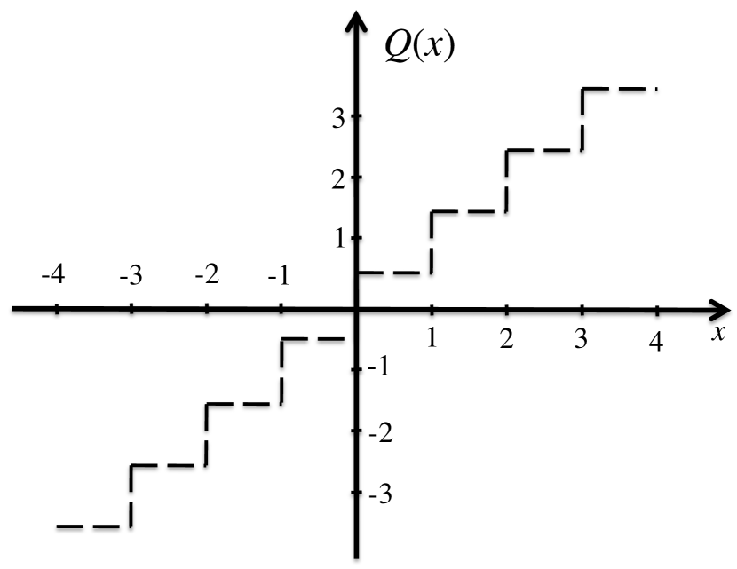
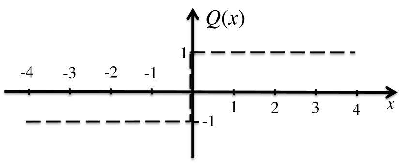
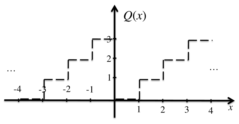
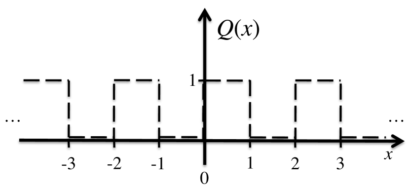
(a)

(b)

(c)

(d)

Figure 1: Examples of Quantization Functions. Typical (a) multibit and (b) binary (1-bit) quantization functions used in scalar quantization. Proposed (c) multibit and (d) binary quantization functions, used in this work.

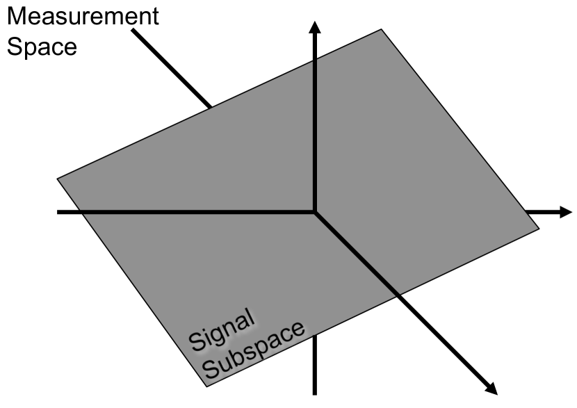
(a)

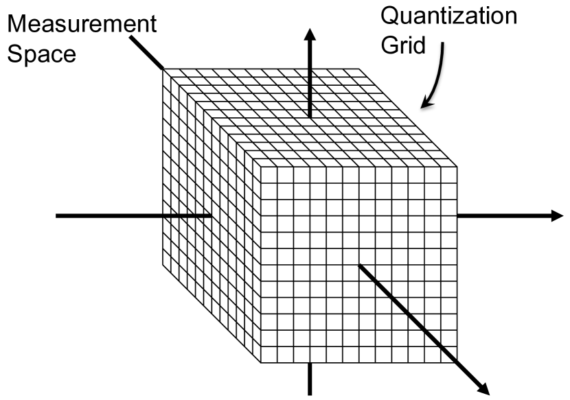
(b)

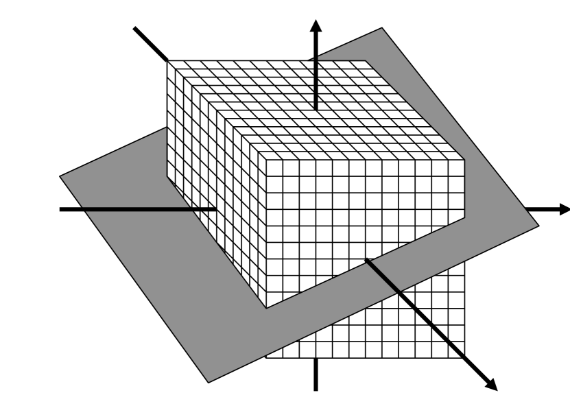
(c)

Figure 2: Oversampled Signals and Quantization. (a) Oversampled signals occupy only a small subspace in the measurement space. (b) The quantization grid quantizes all the measurement space. (c) The signal subspace intersects very few of the available quantization cells.

To overcome the adverse trade-off, a scalar quantizer should be able to use most of the $2^{MB}$ available quantization vectors, i.e., intersect most of the available quantization cells. Note that no-matter how we choose the quantization intervals, the shape of the quantization cells is rectangular and aligned with the axes. Thus, improving the trade-off requires a strategy other than changing the shape and positioning of the quantization cells. The approach we use in this paper is to make the quantization cells non-continuous by making the quantization function non monotonic, as shown in Figs. 1(c) and 1(d). This is, in many ways, similar to the binning of quantization cells explored experimentally in [40]. The advantage of our approach is that it facilitates theoretical analysis and can scale down to even one bit per measurement. In the remainder of this paper we demonstrate that our proposed approach achieves, with very high probability, exponential decay in the worst-case quantization error as a function of the oversampling rate, and, consequently, the bit-rate.

III Rate-efficient Scalar Quantization

III-A Overview

Our approach uses the scalar quantizer described in (1) and (2) with the quantization function in Figs. 1(c) and 1(d). The quantization function is explicitly designed to be non-monotonic, such that non-contiguous quantization regions quantize to the same quantization value. This allows the subspace defined by the measurements to intersect the majority of the available quantization cells which, in turn, ensures efficient use of the available bit-rate. Although we do not describe a specific reconstruction algorithm, we assume that the reconstruction algorithm produces a signal consistent with the measurements, in addition to imposing a signal model or other application-specific requirements.

Our end goal is to determine an upper bound for the probability that there exist two signals $\mathbf{x}$ and $\mathbf{x}^{\prime}$ with distance greater than $d$ that quantize to the same quantization vector given the number of measurements $M$. If no such pair exists, then any consistent reconstruction algorithm will reconstruct a signal that has distance from the acquired signal at most $d$. We wish to demonstrate that this probability vanishes very fast as the number of measurements increases. Furthermore, we wish to show that for a fixed probability of such a signal pair existing, the distance to guarantee such probability decreases exponentially with the number of measurements. An important feature of our development is that the probability of success is on the acquisition system randomization, which we control, and not on any probabilistic model for the signals acquired.

To achieve our goal we first consider a single measurement on a pair of signals $\mathbf{x}$, and $\mathbf{x}^{\prime}$ with distance $d=\|\mathbf{x}-\mathbf{x}^{\prime}\|_{2}$, and analyze the probability a single measurement of the two signals quantizes to the same quantization value for both. Our result is summarized in Lemma III.1.

Lemma III.1

Consider signals $\mathbf{x}$, and $\mathbf{x}^{\prime}$ with $d=\|\mathbf{x}-\mathbf{x}^{\prime}\|_{2}$ and the quantized measurement function

$$q=Q\left(\frac{\langle\mathbf{x},\phi\rangle+w}{\Delta}\right),$$

where $Q(x)=\lceil x\rceil~{}\mod~{}2$, $\phi_{m}\in\mathbb{R}^{K}$ contains i.i.d. elements drawn from a normal distribution with mean 0 and variance $\sigma^{2}$, and $w_{k}$ is i.i.d., uniformly distributed in $[0,\Delta]$.

The probability that the two signals produce equal quantized measurements is

$$P(\mathbf{x},\mathbf{x}^{\prime}\mathrm{~{}consistent}|d)=\frac{1}{2}+\sum_{i=0}^{+\infty}\frac{e^{-\left(\frac{\pi(2i+1)\sigma d}{\sqrt{2}\Delta}\right)^{2}}}{\left(\pi(i+1/2)\right)^{2}}\leq\frac{1}{2}+\frac{1}{2}e^{-\left(\frac{\pi\sigma d}{\sqrt{2}\Delta}\right)^{2}}.$$

We prove this lemma in Sec. III-B.

Next, in Sec. III-C, we consider a single measurement on two $\epsilon$-balls, $\mathcal{B_{\epsilon}({\mathbf{x}})}$ and $\mathcal{B_{\epsilon}({\mathbf{x}^{\prime}})}$, centered at $\mathbf{x}$ and $\mathbf{x}^{\prime}$, i.e., on all the signals of distance less than $\epsilon$ from $\mathbf{x}$ and $\mathbf{x}^{\prime}$. Using Lemma III.1, we lower-bound the probability that no signal in $\mathcal{B_{\epsilon}({\mathbf{x}})}$ is consistent with any signal in $\mathcal{B_{\epsilon}({\mathbf{x}^{\prime}})}$. This leads to Lemma III.2.

Lemma III.2

Consider signals $\mathbf{x}$, and $\mathbf{x}^{\prime}$ with $d=\|\mathbf{x}-\mathbf{x}^{\prime}\|_{2}$, the $\epsilon$-balls $\mathcal{B_{\epsilon}({\mathbf{x}})}$ and $\mathcal{B_{\epsilon}({\mathbf{x}^{\prime}})}$ and the quantized measurement function in Lemma III.1.

The probability that no signal in $\mathcal{B_{\epsilon}({\mathbf{x}})}$ produces equal quantized measurement with any signal in $\mathcal{B_{\epsilon}({\mathbf{x}^{\prime}})}$ (i.e. the probability that the two balls produce inconsistent measurements) is lower bounded by

$$P(\mathcal{B_{\epsilon}({\mathbf{x}})},\mathcal{B_{\epsilon}({\mathbf{x}^{\prime}})}\mathrm{~{}inconsistent}|d)\geq 1-\left(P(\mathbf{x},\mathbf{x}^{\prime}\mathrm{~{}consistent}|d)+\frac{2c_{p}\epsilon}{\Delta}+\gamma\left(\frac{K}{2},\left(\frac{c_{p}}{2\sigma}\right)^{2}\right)\right),$$

for any choice of $c_{P}\leq\Delta/2\epsilon$, where $\gamma(s,x)$ is the regularized upper incomplete gamma function.

Finally we construct a covering of the signal space under consideration using $\epsilon$-balls. We consider all pairs of $\epsilon$-balls in this covering and using Lemma III.2 we lower bound the probability than no pair of signals with distance greater than $d$ produces consistent measurements. This produces the main result of this work, proven in Sec. III-D.

Theorem III.3

Consider the set of signals

$$\mathcal{S}=\left\{\left.\mathbf{x}\in\mathbb{R}^{K}\right|\|\mathbf{x}\|_{2}\leq 1\right\}$$

and the measurement system

$$q_{m}=Q\left(\frac{\langle\mathbf{x},\phi_{m}\rangle+w_{m}}{\Delta}\right),~{}m=1,\ldots,M,$$

where $Q(x)=\lceil x\rceil~{}\mod~{}2$, $\phi_{m}\in\mathbb{R}^{K}$ contains i.i.d. elements drawn from a standard normal distribution, $w_{k}$ is i.i.d., uniformly distributed in $[0,\Delta]$.

For any $c_{r}>1/2$, arbitrarily close to $1/2$, there exists a constant $c_{o}$ and a choice of $\Delta$ proportional to $d$ such that with probability greater than

$$P\geq 1-\left(\frac{c_{o}\sqrt{K}}{d}\right)^{2K}\left(c_{r}\right)^{M}$$

the following holds for all $\mathbf{x},\mathbf{x}^{\prime}\in\mathcal{S}$

$$\|\mathbf{x}-\mathbf{x}^{\prime}\|_{2}\geq d~{}\Rightarrow~{}\mathbf{q}\neq\mathbf{q}^{\prime},$$

where $\mathbf{q}$ and $\mathbf{q}^{\prime}$ are the vectors containing the quantized measurements of $\mathbf{x}$ and $\mathbf{x}^{\prime}$, respectively.

The theorem trades-off the leading term $\left(\frac{c_{o}\sqrt{K}}{d}\right)^{2K}$ with how close to 1/2 is $c_{r}$, i.e., how fast the probability in the statement approaches 1 as a function of the number of measurements. Using an example, we also make this result concrete and show that for $K>8$, we can achieve $c_{o}=60,~{}c_{r}=3/4$.

Our results do not assume a probabilistic model on the signal. Instead they are similar in nature to many probabilistic results in Compressive Sensing [17, 19, 12, 18, 13, 14, 15]. With overwhelming probability the system works on all signals presented to it. It is also important to note that the results are not asymptotic, but hold for finite $K$ and $M$. Further note that the alternative is not that the system provides incorrect result, only that we cannot guarantee that it will provide correct results. Thus, we fix the probability that we cannot guarantee the results to $P_{0}$ and demonstrate the desired exponential decay of the error.

Corollary III.4

Consider the set of signals, the measurement system and the consistent reconstruction process implied by Thm. III.3. With probability greater than

$$P\geq 1-P_{0},$$

the following holds for all $\mathbf{x},\mathbf{x}^{\prime}\in\mathcal{S}$

$$\|\mathbf{x}-\mathbf{x}^{\prime}\|_{2}\geq\frac{c_{o}\sqrt{K}}{P_{0}^{\frac{1}{2k}}}\left(c_{r}\right)^{\frac{M}{2K}}\Rightarrow\mathbf{q}\neq\mathbf{q}^{\prime}$$

The corollary makes explicit the exponential decay of the worst-case error as a function both of the number of measurements $M$ and the number of bits used. This means that the worst-case error decays significantly faster than the linear decay demonstrated with classical quantization of oversampled frames[1, 3] and defeats the lower bound in [2]. Furthermore, we achieve that rate by quantizing each coefficient independently, unlike existing approaches [8, 39]. Since this is a probabilistic result on the system probability space, it further implies that a system that satisfies the desired exponential decay property exists.

One of the drawbacks of this approach is that it requires the quantizer to be designed in advance with the target distortion in mind, i.e., the choice of the scaling parameter $\Delta$ of the quantizer affects the distortion. This might be an issue if the target accuracy and oversampling rate is not known at the quantizer design stage, but, for example, needs to be estimated from the measurements adaptively during measurement time. This drawback, as well as one way to overcome it, is discussed further in Sec. V.

The remainder of this section presents the above results in sequence.

III-B Quantized Measurement of Signal Pairs

We first consider two signals $\mathbf{x}$ and $\mathbf{x}^{\prime}$ with $\ell_{2}$ distance $d=\|\mathbf{x}-\mathbf{x}^{\prime}\|_{2}$. We analyze the probability that a single quantized measurement of the two signals produces the same bit values, i.e., is consistent for the two signals. Since we only discuss the measurement of a single bit, we omit the subscript $m$ from (1) and (2) to simplify the notation in the remainder of this section. The analysis does not depend on it. We use $q$ and $q^{\prime}$ to denote a single quantized measurement of $\mathbf{x}$ and $\mathbf{x}^{\prime}$, respectively.

We first consider the desired probability conditional on the projected distance $l$, i.e., the distance between the measurements of the signals

$$l \equiv|y-y^{\prime}|=|\langle\mathbf{x},\phi\rangle+w-(\langle\mathbf{x}^{\prime},\phi\rangle+w)|$$

$$\Rightarrow l =|\langle\mathbf{x}-\mathbf{x}^{\prime},\phi\rangle|$$ (7)

The addition of dither makes the probability the two signals quantize to consistent bits depend only on the distance $l$ and not on the individual values $y$, and $y^{\prime},$ as demonstrated in Fig. 3(a). In the top part of the figure an example measurement is depicted. Depending on the amount of dither, the two measurements can quantize to different values (as shown in the second line of the plot) or to the same values (as shown in the third line). Since the dither is uniform in $[0,\Delta]$, the probability the two bits are consistent given $l$ equals

$$P(q=q^{\prime}|l)=\left\{\begin{array}[]{rcr}1-\frac{l\mod\Delta}{\Delta}=1+2i-\frac{l}{\Delta},&\mathrm{if}&2i\Delta\leq l\leq(2i+1)\Delta\\ \frac{l\mod\Delta}{\Delta}=\frac{l}{\Delta}-(2i+1),&\mathrm{if}&(2i+1)\Delta\leq l\leq 2(i+1)\Delta,\end{array}\right.$$ (10)

for some integer $i$, which is plotted in Fig. 3(b).

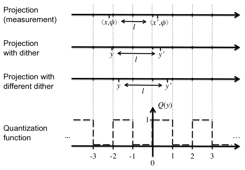
(a)

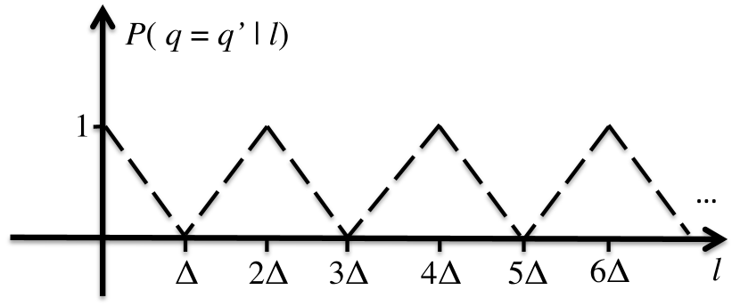
(b)

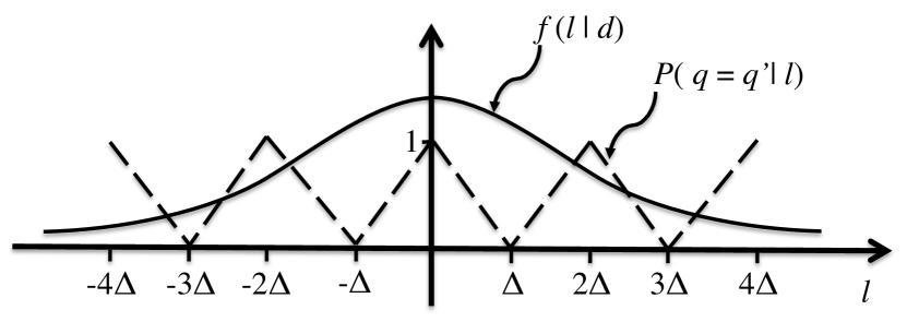
(c)

Figure 3: Analysis of the probility of consistency for a single bit. (a) Dithering makes this probability depend only on the distance between the two signals. (b) Probability of consistency as a function of the projection length. (c) The two components affecting the overall probability of consistency.

Furthermore, from (7) and the distribution of $\phi$, it follows that $l$ is distributed as the magnitude of the normal distribution with variance $(\sigma d)^{2}$

$$f(l|d)=\sqrt{\frac{2}{\pi}}\frac{e^{-\left(\frac{l}{2\sigma d}\right)^{2}}}{\sigma d},~{}l\geq 0.$$

Thus, the two quantization bits are the same given the distance of the signals $d$ with probability

$$P(q=q^{\prime}|d)=\int_{l\geq 0}P(q=q^{\prime}|l)\cdot f(l|d)\mathrm{d}l.$$ (11)

In order to evaluate the integral, we make it symmetric around zero by mirroring it and dividing it by two. The two components of the expanded integral are shown in Fig. 3(c). These are a periodic triangle function with height 1 and width $2\Delta$ and a Normal distribution function with variance $(\sigma d)^{2}$.

Using Parseval’s theorem, we can express that integral in the Fourier domain (with respect to $l$). Noting that the periodic triangle function can also be represented as a convolution of a single triangle function with an impulse train, we obtain:

$$P(q=q^{\prime}|d) =\int_{\xi}\stackrel{{\scriptstyle P(q=q^{\prime}|l)}}{{\overbrace{\frac{1}{2}\sum_{i=-\infty}^{+\infty}\mathrm{sinc}^{2}\left(\frac{i}{2}\right)\delta\left(\xi-\frac{i}{2\Delta}\right)}}}\stackrel{{\scriptstyle f(l|d)}}{{\overbrace{e^{-2(\pi\xi\sigma d)^{2}}}}}\mathrm{d}\xi$$

$$=\sum_{i=-\infty}^{+\infty}\frac{\mathrm{sinc}^{2}\left(\frac{i}{2}\right)}{2}e^{-\left(\frac{\pi i\sigma d}{\sqrt{2}\Delta}\right)^{2}}$$

where $\mathrm{sinc}(x)\equiv\frac{\sin(\pi x)}{\pi x}$, and $\xi$ is the frequency with respect to $l$. Since $\mathrm{sinc}(x)=0$ if $x$ is a non-zero integer, $\sin^{2}(\pi x/2)=1$ if $x$ is an odd integer, and $\mathrm{sinc}(0)=1$,

$$P(q=q^{\prime}|d) =\frac{1}{2}+\sum_{i=0}^{+\infty}\frac{e^{-\left(\frac{\pi(2i+1)\sigma d}{\sqrt{2}\Delta}\right)^{2}}}{\left(\pi(i+1/2)\right)^{2}},$$ (12)

which proves the equality in Lemma III.1.

A very good lower bound for (12) can be derived using the first term of the summation:

$$P(q=q^{\prime}|d) \geq\frac{1}{2}+\frac{4}{\pi^{2}}e^{-\left(\frac{\pi\sigma d}{\sqrt{2}\Delta}\right)^{2}}$$

An alternative lower bound can also be derived by explicitly integrating (11) up to $l\leq\Delta$:

$$P(q=q^{\prime}|d) \geq 1-\sqrt{\frac{2}{\pi}}\frac{\sigma d}{\Delta}$$

An upper bound can be derived using $e^{-\left(\frac{\pi(2i+1)\sigma d}{\sqrt{2}\Delta}\right)^{2}}\leq e^{-\left(\frac{\pi\sigma d}{\sqrt{2}\Delta}\right)^{2}}$ in the summation in (12), and noting that $P(q=q^{\prime}|d=0)=1$.

$$P(q=q^{\prime}|d) \leq\frac{1}{2}+\frac{1}{2}e^{-\left(\frac{\pi\sigma d}{\sqrt{2}\Delta}\right)^{2}},$$

which proves the inequality and concludes the proof of Lemma III.1. Fig. 4 plots these bounds and illustrates their tightness. A bound for the probability of inconsistency can be determined from the bounds above using $P(q\neq q^{\prime}|d)=1-P(q=q^{\prime}|d)$.

Using these results it is possible to further analyse the performance of this method on finite sets of signals. However, for many signal processing applications it is desirable to analyse infinite sets of signals, such as signal spaces. To facilitate this analysis the next section examines how the system behaves on pairs of $\epsilon$-balls in the signal space.

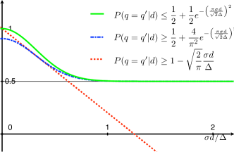
Figure 4: Upper and lower bounds for the probability two different signals have consistent quantization bits

III-C Consistency of $\epsilon$-Balls

In this section we examine the performance on pairs of sets of signals. Specifically, the sets we consider are $\epsilon$-balls in $\mathbb{R}^{K}$ with radius $\epsilon$ and centered at $\mathbf{x}$, defined as

$$\mathcal{B_{\epsilon}({\mathbf{x}})}=\left\{\left.\mathbf{s}\in\mathbb{R}^{K}\right|\|\mathbf{s}-\mathbf{x}\|_{2}\leq\epsilon\right\}.$$

We examine balls $\mathcal{B_{\epsilon}({\mathbf{x}})}$ and $\mathcal{B_{\epsilon}({\mathbf{x}^{\prime}})}$ around two signals $\mathbf{x}$ and $\mathbf{x}^{\prime}$ with distance $d=\|\mathbf{x}-\mathbf{x}^{\prime}\|_{2}$, as above. We desire to lower bound the probability that the quantized measurements of all the signals in $\mathcal{B_{\epsilon}({\mathbf{x}})}$ are consistent with each other, and inconsistent with the ones from all the signals in $\mathcal{B_{\epsilon}({\mathbf{x}^{\prime}})}$.

To determine the lower bound, we examine how the measurement vector $\phi$ affects the $\epsilon$-balls. It is straightforward to show that the measurement projects the $\mathcal{B_{\epsilon}({\mathbf{x}})}$ to an interval in $\mathbb{R}$ of length at most $2\epsilon\|\phi\|_{2}$, centered at $\langle\mathbf{x},\phi\rangle$. The length of the interval affects the probability that the measurements of all the signals in $\mathcal{B_{\epsilon}({\mathbf{x}})}$ quantize consistently. To guarantee consistency we bound the length of this interval to be smaller than $2c_{p}\epsilon$, i.e., we require that $\|\phi\|_{2}\leq c_{p}$. This fails with probability

$$P(\|\phi\|_{2}\geq c_{p}) =\gamma\left(\frac{K}{2},\left(\frac{c_{p}}{2\sigma}\right)^{2}\right),$$

where $\gamma(s,x)$ is the regularized upper incomplete gamma function, and $\gamma\left(\frac{K}{2},\left(\frac{x}{2}\right)^{2}\right)$ is the tail integral of the $\chi$ distribution with $K$ degrees of freedom (i.e., the distribution of the norm of a $K$-dimensional standard Gaussian vector). To ensure that all the signals in the $\epsilon$-ball can quantize to the same bit value with non-zero probability we pick $c_{p}$ such that $2c_{p}\epsilon<\Delta$.

Under this restriction, the two balls will produce inconsistent measurements only if the two intervals they project onto are located completely within two quantization intervals with different quantization values. Thus we cannot guarantee consistency within the ball if the ball projection is on the boundary of a quantization threshold, and we cannot guarantee inconsistency between the balls if parts of the projections of the two balls quantize to the same bit. Figure 5(b) demonstrates the quantization of $\epsilon$-balls, and examines when all the elements of the two balls quantize inconsistently.

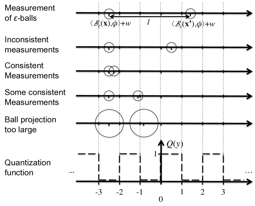
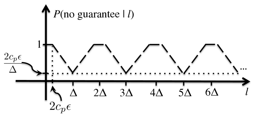
(a)

(b)

Figure 5: Measurement quantization of $\epsilon$-balls. (a) Ball measurement and consistency behavior. (b) Probability of no consistency guarantee given the projection length, (16).

Assuming that the width of the ball projections is bounded, as described above, then we can characterize the probability that the ball centers will project on the quantization grid in a way that all signals within one ball quantize to the same one quantization value, and all the signals from the other ball quantize to the other. This is the probability that we can guarantee that all measurements from the signals in one ball are inconsistent with all the signals from the other ball. We desire to upper bound the probability that we fail to guarantee this inconsistency.

Using, as before, $l$ to denote the projected distance between the two centers of the balls, we cannot guarantee inconsistency if $|l-2i\Delta|\leq 2c_{p}\epsilon$ for some $i$. In this case the balls are guaranteed to intersect modulo $2\Delta$, i.e., they are guaranteed to have intervals that quantize to the same value. If $2c_{p}\epsilon\leq l-2i\Delta\leq\Delta$ for some $i$ we consider the projection of the balls and the two points, one from each projection, closest to each other. If these, which have distance $l-2c_{p}\epsilon$ modulo $2\Delta$, are inconsistent, then the two balls are guaranteed to be inconsistent. Similarly, if $0\leq l-(2i+1)\Delta\leq\Delta-2c_{p}\epsilon$ for some $i$ we consider the projection of the balls and the two points, one from each projection, farthest from each other. If these, which have distance $l+2c_{p}\epsilon$ modulo $2\Delta$, are inconsistent, then the two balls are guaranteed to be inconsistent. Since, given $l$, the dither distributes the centers of the balls uniformly within the quantization intervals, the probability that we cannot guarantee consistency can be bounded in a manner similar to (10).

$$P(\mathrm{no~{}guarantee}|l) \leq\left\{\begin{array}[]{rl}1,&\mbox{if~{}}|l-2i\Delta|\leq 2c_{p}\epsilon\\ \frac{\Delta+2c_{p}\epsilon-l-2i\Delta}{\Delta},&\mbox{if~{}}2c_{p}\epsilon\leq l-2i\Delta\leq\Delta\\ \frac{l+2c_{p}e-(2i+i)\Delta}{\Delta},&\mbox{if~{}}0\leq l-(2i+1)\Delta\leq\Delta-2c_{p}\epsilon,\\ \end{array}\right.$$ (16)

for some integer $i$. The shape of this upper bound is shown in Fig. 5(b). Note that the right hand side of (16) can be expressed in terms of $P(q=q^{\prime}|l)$ from (10) to produce

$$P\left(\mathrm{no~{}guarantee}|d\right) \leq\min\left\{P\left(q=q^{\prime}|d\right)+\frac{2c_{p}\epsilon}{\Delta},1\right\}$$

$$\leq P\left(q=q^{\prime}|d\right)+\frac{2c_{p}\epsilon}{\Delta}.$$

Thus we can upper bound the probability of inconsistent measurements due to either a large ball projection interval or due to unfavorable projection of the ball centers using the union bound.

$$P\left(\exists~{}\mathbf{v}\in\mathcal{B_{\epsilon}({\mathbf{x}})},\mathbf{v}^{\prime}\in\mathcal{B_{\epsilon}({\mathbf{x}^{\prime}})},\mathrm{~{}s.t.~{}}q_{\mathbf{v}}=q_{\mathbf{v}^{\prime}}|d\right) \leq P\left(\mbox{no guarantee}|d\right)+P\left(\|\phi\|_{2}\geq c_{p}\right)$$

$$\leq P\left(q=q^{\prime}|d\right)+\frac{2c_{p}\epsilon}{\Delta}+\gamma\left(\frac{K}{2},\left(\frac{c_{p}}{2\sigma}\right)^{2}\right),$$

where $q_{\mathbf{v}}$ and $q_{\mathbf{v}^{\prime}}$ are the quantization values of $\mathbf{v}$, and $\mathbf{v}^{\prime}$, respectively. This proves Lemma III.2.

III-D Consistency Of $M$ Measurements For All Signals In The Space

To determine the overall quantization performance, we consider bounded norm signals $\mathbf{x}$ in a $K$ dimensional signal space. Without loss of generality, we assume $\|\mathbf{x}\|_{2}\leq 1$, and denote the set of all such signals using $\mathcal{S}=\left\{\mathbf{x}\in\mathbb{R}^{K},\|\mathbf{x}\|_{2}\leq 1\right\}$. To consider all the points in $\mathcal{S}$ we construct a covering using $\epsilon$-balls, such that any signals in $\mathcal{S}$ belongs to at least one such ball. The minimum number of balls required to cover a signal set is the covering number of the set. For the unit ball in $K$ dimensions, the covering number is $C_{\epsilon}\leq(3/\epsilon)^{K}$ $\epsilon$-balls [15].

Next, we consider all pairs of balls $(\mathcal{B_{\epsilon}({\mathbf{x}})},\mathcal{B_{\epsilon}({\mathbf{x}^{\prime}})})$, such that $\|\mathbf{x}-\mathbf{x}^{\prime}\|_{2}\geq d$. The number of those is upper bounded by the total number of pairs of $\epsilon$-balls we can form from the covering, independent of the distance of their centers, namely $\binom{C_{\epsilon}}{2}\leq C_{\epsilon}^{2}$ pairs. The probability that at least one pair of vectors, one from each ball has $M$ consistent measurements is upper bounded by

$$P(M\mathrm{~{}measurements~{}consistent}|d) =P(\exists~{}\mathbf{v}\in\mathcal{B_{\epsilon}({\mathbf{x}})},\mathbf{v}^{\prime}\in\mathcal{B_{\epsilon}({\mathbf{x}^{\prime}})},\mathrm{~{}s.t.~{}}\mathbf{q}_{\mathbf{v}}=\mathbf{q}_{\mathbf{v}^{\prime}}|d)$$

$$\leq P(\exists~{}\mathbf{v}\in\mathcal{B_{\epsilon}({\mathbf{x}})},\mathbf{v}^{\prime}\in\mathcal{B_{\epsilon}({\mathbf{x}^{\prime}})},\mathrm{~{}s.t.~{}}q_{\mathbf{v}}=q_{\mathbf{v}^{\prime}}|d)^{M}$$

Thus, the probability that there exists at least one pair of balls that contains at least one pair of vectors, one from each ball, that quantize to $M$ consistent measurements can be upper bounded using the union bound

$$P(\exists~{}\mathbf{x},\mathbf{x}^{\prime}\in\mathcal{S},\|\mathbf{x}-\mathbf{x}^{\prime}\|_{2}>d~{}\mbox{s.t.}~{}\mathbf{q}=\mathbf{q}^{\prime}) \leq\left(\frac{3}{\epsilon}\right)^{2K}P(M\mathrm{~{}measurements~{}consistent}|d)$$

It follows that the probability that we cannot guarantee inconsistency for all vectors with distance greater than $d$ is upper bounded by

$$P(\exists~{}\mathbf{x},\mathbf{x}^{\prime}\in\mathcal{S},\|\mathbf{x}-\mathbf{x}^{\prime}\|_{2}>d~{}\mbox{s.t.}~{}\mathbf{q}=\mathbf{q}^{\prime}) \leq\left(\frac{3}{\epsilon}\right)^{2K}\left(P(q=q^{\prime}|d)+\frac{2c_{p}\epsilon}{\Delta}+\gamma\left(\frac{K}{2},\left(\frac{c_{p}}{2\sigma}\right)^{2}\right)\right)^{M}$$

$$\leq\left(\frac{3}{\epsilon}\right)^{2K}\left(\frac{1}{2}+\frac{1}{2}e^{-\left(\frac{\pi\sigma d}{\sqrt{2}\Delta}\right)^{2}}+\frac{2c_{p}\epsilon}{\Delta}+\gamma\left(\frac{K}{2},\left(\frac{c_{p}}{2\sigma}\right)^{2}\right)\right)^{M}.$$

Picking $\sigma=\frac{1}{\sqrt{K}},~{}\epsilon=\frac{\Delta r_{1}}{2c_{p}}$, and $\Delta=\frac{dr_{2}}{\sqrt{K}}$ for some ratios $r_{1},r_{2}>0$ we obtain

$$P(\exists~{}\mathbf{x},\mathbf{x}^{\prime}\in\mathcal{S},\|\mathbf{x}-\mathbf{x}^{\prime}\|_{2}>d~{}\mbox{s.t.}~{}\mathbf{q}=\mathbf{q}^{\prime}) \leq\left(\frac{\sqrt{K}}{d}\frac{6c_{p}}{r_{1}r_{2}}\right)^{2K}\left(\frac{1}{2}+\frac{1}{2}e^{\frac{-\pi^{2}}{2r_{2}^{2}}}+r_{1}+\gamma\left(\frac{K}{2},\frac{c_{p}^{2}K}{4}\right)\right)^{M},$$

By setting $c_{p}$ arbitrarily large, and $r_{1}$ and $r_{2}$ arbitrarily small, we can achieve

$$P(\exists~{}\mathbf{x},\mathbf{x}^{\prime}\in\mathcal{S},\|\mathbf{x}-\mathbf{x}^{\prime}\|_{2}>d~{}\mbox{s.t.}~{}\mathbf{q}=\mathbf{q}^{\prime}) \leq\left(\frac{c_{o}\sqrt{K}}{d}\right)^{2K}\left(c_{r}\right)^{M},$$

where $c_{o}=6c_{p}/r_{1}r_{2}$ increases as $c_{r}$ decreases, and $c_{r}$ can be any constant arbitrarily close to 1/2. This proves Thm. III.3. Corollary III.4 follows trivially.

For example, to make this result concrete, if $K>8$ we can pick $c_{p}=2,~{}\epsilon=\frac{\Delta}{20}$, and $\Delta=\frac{d}{\sqrt{K}}$ to obtain:

$$P(\exists~{}\mathbf{x},\mathbf{x}^{\prime}\in\mathcal{S},\|\mathbf{x}-\mathbf{x}^{\prime}\|_{2}>d~{}\mbox{s.t.}~{}\mathbf{q}=\mathbf{q}^{\prime}) \leq\left(\frac{60\sqrt{K}}{d}\right)^{2K}\left(\frac{3}{4}\right)^{M}=e^{2K\log\left(\frac{60\sqrt{K}}{d}\right)-M\log\left(\frac{4}{3}\right)}.$$

We should remark that the choice of parameters $r_{1},r_{2}$ at the last step—which also determines the design of the precision parameter $\Delta$—influences the decay rate of the error, at a trade-off with the leading constant term. While we can obtain a decay rate arbitrarily close to $1/2$, we will also force the leading term $(c_{o}\sqrt{K}/d)^{2K}$ to become arbitrarily large. As mentioned before, the decision to decrease $\Delta$ should be done at design time. Furthermore, decreasing $\Delta$ can be difficult in certain practical hardware implementations.

The $\sqrt{K}$ factor is consistent with scalar quantization of orthonormal basis expansions. Specifically, consider the orthonormal basis expansion of the signal, quantized to $B$ bits per coefficient for a total of $KB$ bits. The worst-case error per coefficient is $2^{-(B-1)}$ and, therefore, the total worst-case error is $2^{-(B-1)}\sqrt{K}$.

To better understand the result, we examine how many bits we require to achieve the same performance as fine scalar quantization of orthonormal basis expansions. To provide the same error guarantee we set $d=2^{-(B-1)}\sqrt{K}$. Using Corollary III.4, to achieve this guarantee with probability $P_{0}$ we require

$$2^{-(B-1)}\sqrt{K} \geq\frac{c_{o}\sqrt{K}}{P_{0}^{\frac{1}{2K}}}\left(c_{r}\right)^{\frac{M}{2K}}$$

$$\Rightarrow\frac{M}{K} \geq\left.2\left(B\log 2+\log\frac{c_{o}}{2P_{0}^{\frac{1}{2K}}}\right)\right/\log\left(1/c_{r}\right).$$

Thus the number of bits per dimension $M/K$ required grows linearly with the bits per dimension $B$ required to achieve the same error guarantee in an orthonormal basis expansion. The oversampled approach asymptotically requires $2\log(2)/\log(1/c_{r})$ times the number of bits per dimension, compared to fine quantization of orthonormal basis expansions, an overhead which can be designed to be arbitrarily close to 2 times. For our example $c_{r}=3/4$, $2\log(2)/\log(1/c_{r})\approx 4.82$. Although this penalty is significant, it is also significantly improved over classical scalar quantization of oversampled expansions.

IV Quantization Universality and Signal Models

IV-A Universality and Side Information

One of the advantage of our approach is its universality, in the sense that we did not use any information on the signal model in designing the quantizer. This is a significant advantage of randomized sampling methods, such as Johnson-Lindenstrauss embedding and Compressive Sensing [41, 42, 20, 13]. Additional information about the signal can be exploited in the reconstruction to improve performance.

The information available about the signal can take the form of a model on the signal structure, e.g., that the signal is sparse, or that it lies in a manifold [13, 43, 44, 45, 46, 47]. Alternatively, we might have prior knowledge of an existing signal that is very similar to the acquired one (e.g., see [48]). This information can be incorporated in the reconstruction to improve the reconstruction quality. It is expected that such information can allow us to provide stronger guarantees for the performance of our quantizer.

We incorporate side information by modifying the set $\mathcal{S}$ of signals of interest. This set affects our performance through the number of $\epsilon$-balls required to cover it, known as the covering number of the set. In the development above, for $K$-dimensional signals with norm bounded by 1, covering can be achieved by $C_{\epsilon}=(3/\epsilon)^{K}$ balls. The results we developed, however, do not rely on any particular covering number expression. In general, any set $\mathcal{S}$ can be quantized successfully with probability

$$P(\exists~{}\mathbf{x},\mathbf{x}^{\prime}\in\mathcal{S},\|\mathbf{x}-\mathbf{x}^{\prime}\|_{2}>d~{}\mbox{s.t.}~{}\mathbf{q}=\mathbf{q}^{\prime}) \leq C_{3d/c_{o}\sqrt{K}}^{\mathcal{S}}\left(c_{r}\right)^{M},$$

where $C_{\epsilon}^{\mathcal{S}}$ denotes the covering number of the set of interest $\mathcal{S}$ as a function of the ball size $\epsilon$, and $c_{o},c_{r}$ are as defined above.

This observation allows us to quantize known classes of signals, such as sparse signals or signals in a union of subspaces. All we need for this characterization is an upper bound for the covering number of the set (or its logarithm, i.e., the Kolmogorov $\epsilon$-entropy of the set [49]). The underlying assumption is the same as above: that the reconstruction algorithm selects a signal in the set $\mathcal{S}$ that is consistent with the quantized measurements.

The Kolmogorov $\epsilon$-entropy of a set provides a lower bound on the number of bits necessary to encode the set with worst case distortion $\epsilon$ using vector quantization. To achieve this rate, we construct the $\epsilon$-covering of the set and use the available bits to enumerate the centers of the $\epsilon$-balls comprising the covering. Each signal is quantized to the closest $\epsilon$-ball center, the index of which is used to represent the signal. While the connection with vector quantization is well understood in the literature, the results in this paper provide, to our knowledge, the first example relating the Kolmogorov $\epsilon$-entropy of a set and the achievable performance under scalar quantization. Specifically, using a similar derivation to Cor. III.4, the number of bits sufficient to guarantee worst-case distortion $d$ with probability greater than $1-P_{0}$ is

$$M\geq\frac{\log C_{3d/c_{o}\sqrt{K}}^{\mathcal{S}}+\log\frac{1}{P_{0}}}{\log\frac{1}{c_{r}}},$$ (17)

where $\log C_{3d/c_{o}\sqrt{K}}^{\mathcal{S}}$ is the $\epsilon$-entropy for $\epsilon=3d/c_{o}\sqrt{K}$. Aside from constants, there is a $\sqrt{K}$ penalty over vector quantization in our approach, consistent with the findings in Sec. III-D.

In the remainder of this section we examine three special cases: Compressive Sensing, signals in a union of subspaces, and signals with a known similar signal as side information.

IV-B Quantization of Sparse Signals

Compressive Sensing, one of the recent developments in signal acquisition technology, assumes that the acquired signal $\mathbf{x}$ contains few non-zero coefficients, i.e., is sparse, when expressed in some basis. This assumption significantly reduces the number of measurements required for acquisition and exact reconstruction [13, 17, 19, 20]. However, when combined with scalar quantization it can be shown that CS measurements are quite inefficient in terms of their rate-distortion trade-off [25]. The cause is essentially the same as the cause for the inefficiency of oversampling in the case of non-sparse signals: sparse signals occupy a small number of subspaces in the measurement space. Thus, they do not intersect most of the available quantization points. The proposed quantization scheme has the potential to significantly improve the rate-distortion performance of CS.

Compressive Sensing examines $K$-sparse signals in an $N$-dimensional space. Thus the signal acquired contains up to $K$ non-zero coefficients and, therefore, lies in a $K$-dimensional subspace out of the $\binom{N}{K}$ such subspaces. Since each of the subspaces can be covered with $(3/\epsilon)^{K}$ balls, and picking $\sigma=\frac{1}{\sqrt{N}},~{}\epsilon=\frac{\Delta r_{1}}{2c_{p}}$, and $\Delta=\frac{dr_{2}}{\sqrt{N}}$, the probabilistic guarantee of reconstruction becomes

$$P(\exists~{}\mathbf{x},\mathbf{x}^{\prime}\in\mathcal{S},\|\mathbf{x}-\mathbf{x}^{\prime}\|_{2}>d~{}\mbox{s.t.}~{}\mathbf{q}=\mathbf{q}^{\prime}) \leq\binom{N}{K}^{2}\left(\frac{c_{o}\sqrt{N}}{d}\right)^{2K}\left(c_{r}\right)^{M}$$

$$\leq\left(\frac{eN^{3/2}}{K}\frac{c_{o}}{d}\right)^{2K}\left(c_{r}\right)^{M}$$

$$\leq e^{2K\log\left(\frac{eN^{3/2}}{K}\frac{c_{o}}{d}\right)-M\log(1/c_{r})}$$

which decays exponentially with $M$, as long as $M=\Omega\left(K\log N-K\log\left(Kd\right)\right)=\Omega\left(K\log\left(N/Kd\right)\right)$, similar to most Compressive Sensing results. The difference here is that there is an explicit rate-distortion guarantee since $M$ represents both the number of measurements and the number of bits used.

IV-C Quantization of Signals in a Union of Subspaces

A more general model is signals in a finite union of subspaces[43, 44, 45, 46]. Under this model, the signal being acquired belongs to one of $L$ $K$-dimensional subspaces. In this case the reconstruction guarantee becomes

$$P(\exists~{}\mathbf{x},\mathbf{x}^{\prime}\in\mathcal{S},\|\mathbf{x}-\mathbf{x}^{\prime}\|_{2}>d~{}\mbox{s.t.}~{}\mathbf{q}=\mathbf{q}^{\prime}) \leq L^{2}\left(\frac{c_{o}\sqrt{N}}{d}\right)^{2K}\left(c_{r}\right)^{M}$$

$$\leq e^{2\log L+2K\log\left(\frac{c_{o}\sqrt{N}}{d}\right)-M\log(1/c_{r})},$$

which decays exponentially with $M$, as long as $M=\Omega(\log L+K\log(N/d))$. Compressive Sensing is a special case of signals in a union of subspaces, where $L=\binom{N}{K}$.

This result is in contrast with the analysis on unquantized measurement for signals in a union of subspaces [43, 44, 45, 46]. Specifically, these results demonstrate no dependence on, $N$, the size of the ambient signal space; $O(\log L+K)$ unquantized measurements are sufficient to robustly reconstruct signals from a union of subspaces. On the other hand, using an analysis similar to [2, 25] it is straightforward to show that increasing the rate by increasing the number of measurements provides only a linear reduction of the error as a function of the number of measurements, similar to the behavior described by (6). Alternatively, we can consider the Kolmogorov $\epsilon$-entropy, i.e., the minimum number of bits necessary to represent the signal set at distortion $\epsilon$, without requiring robustness or imposing linear measurements. This is exactly equal to $\log_{2}\left(C_{\epsilon}^{\mathcal{S}}\right)$ and suggests that $O(\log L+K)$ bits are required. Whether the logarithmic dependence on $N$ exhibited by our approach is fundamental, due to the requirement for linear measurements, or whether it can be removed by different analysis is an interesting question for further research.

IV-D Quantization of Similar Signals

Quite often, the side information is a known signal $\mathbf{x}_{s}$ that is very similar to the acquired signal. For example, in video applications one frame might be very similar to the next; in multispectral image acquisition and compression the acquired signal in one spectral band is very similar to the acquired signal in another spectral band [48]. In such cases, knowledge of $\mathbf{x}_{s}$ can significantly reduce the number of quantized measurements required to acquire the new signal.

As an example, consider the case where it is known that the acquired signal $\mathbf{x}$ differs from the side information $\mathbf{x}_{s}$ by at most $D\geq\|\mathbf{x}_{s}-\mathbf{x}\|_{2}$. Thus the acquired signal exists in the $D$-ball around $\mathbf{x}_{s}$, $\mathcal{B_{D}({\mathbf{x}_{s}})}$. Using the same argument as above, we can construct a covering of a $D$-ball using $(3D/\epsilon)^{K}$$\epsilon$-balls. Thus, the distortion guarantee becomes

$$P(\exists~{}\mathbf{x},\mathbf{x}^{\prime}\in\mathcal{S},\|\mathbf{x}-\mathbf{x}^{\prime}\|_{2}>d~{}\mbox{s.t.}~{}\mathbf{q}=\mathbf{q}^{\prime}) \leq\left(\frac{c_{o}D\sqrt{K}}{d}\right)^{2K}\left(c_{r}\right)^{M}.$$

If we fix the probability that we fail to guarantee reconstruction performance to $P_{0}$, as with Cor. III.4, the distorition guarantee we can provide decreases linearly with $D$.

$$\|\mathbf{x}-\mathbf{x}^{\prime}\|_{2}\geq\frac{c_{o}D\sqrt{K}}{P_{0}^{\frac{1}{2k}}}\left(c_{r}\right)^{\frac{M}{2K}}\Rightarrow\mathbf{q}\neq\mathbf{q}^{\prime}.$$

V Discussion and open questions

This paper demonstrates universal scalar quantization with exponential decay of the quantization error as a function of the oversampling rate (and, consequently, of the bit rate). This allows rate-efficient quantization for oversampled signals without any need for methods requiring feedback or joint quantization of coefficients, such as Sigma-Delta or vector quantization. The framework we develop is universal and can incorporate side information on the signal, when available. Our development establishes a direct connection between the Kolmogorov $\epsilon$-entropy of the measured signals and the achievable rate vs. distortion performance under scalar quantization.

The fundamental realization to enable this performance is that continuous quantization regions (i.e., monotonic scalar quantization functions) cause the inherent limitation of scalar quantizers. Using non-continuous quantization regions we make more effective use of the quantization bits. While in this paper we only analyze binary quantization, it is straightforward to analyze multibit quantizers, shown in Fig. 1(c). The only difference is the probability $P(q=q^{\prime}|l)$ that two arbitrary signals produce a consistent measurement in (10) and Fig. 3(b). The modified function should be equal to zero in the intervals $[(2^{B}i+1)\Delta,(2^{B}(i+1)-1)\Delta],i=0,1,\ldots$, and equal to (10) everywhere else. The remaining derivation is identical to the one we presented. We can conjecture that careful analysis of the multibit case should present an exponential decay constant $c_{r}\gtrsim 1/2^{B}$, which can reach that lower bound arbitrarily close.

One of the issues not addressed in this work is practical reconstruction algorithms. Reconstruction from the proposed sampling scheme is indeed not straightforward. However, we believe that our work opens the road to a variety of scalar quantization approaches which can exhibit practical and efficient reconstruction algorithms. One approach is to use the results in this paper hierarchically, with a different scaling parameter $\Delta$ at each hierarchy level, and, therefore, different reconstruction accuracy guarantees. The parameters can be designed such that the reconstruction problem at each level is a convex problem, therefore tractable. This approach is explored in more detail in [50]. We defer discussion of other practical reconstruction approaches to future work.

A difficulty in implementing the proposed approach is that the precision parameter $\Delta$ is tightly related to the hardware implementation of the quantizer. It is also critical to the performance. If the hardware is not precise enough to scale $\Delta$ and produce a fine enough quantization function $Q(x)$, then the asymptotic performance of the quantizer degrades. This is generally not an issue in software implementations, e.g., in compression applications, assuming we do not reach the limits of machine precision.

The precision parameter $\Delta$ also has to be designed in advance to accommodate the target accuracy. This might be undesirable if the required accuracy of the acquisition system is not known in advance, and we hope to decide the number of measurements during the system’s operation, maybe after a certain number of measurements has already been acquired with a lower precision setting. One approach to address this issue is to hierarchically scale the precision parameter, such that the measurements are more and more refined as more are acquired. The hierarchical quantization discussed in [50] implements this approach.

Another topic worthy of further research is performance in the presence of noise. Noise can create several problems, such as incorrect quantization bits. Even with infinite quantization precision, noise in an inescapable fact of signal acquisition and degrades performance. There are several ways to account for noise in this work. One possibility is to limit the size of the precision parameter $\Delta$ such that the probability the noise causes the measurement to move by more than $\Delta$ can be safely ignored. This will limit the number of bit flips due to noise, and should provide some performance guarantee. It will also limit the asymptotic performance of the quantizer. Another possibility is to explore the robust embedding properties of the acquisition process, similar to [33]. More precise examination is an open question, also for future work.

An interesting question is the “democratic” property of this quantizer, i.e. how well the information is distributed to each quantization bit [51, 52, 23]. This is a desirable property since it provides robustness to erasures, something that overcomplete representations are known for [36, 38]. Superficially it seems that the quantizer is indeed democratic. In a probabilistic sense, all the measurements contain the same amount of information. Similarities with democratic properties in Compressive Sensing [52] hint that the democratic property of our method should be true in an adversarial sense as well. However, we have not attempted a proof in this paper.

Last, we should note that this quantization approach has very tight connections with locality-sensitive hashing (LSH) and $\ell_{2}$ embeddings under the hamming distance (e.g., see [53] and references within). Specifically, our quantization approach effectively constructs such an embedding, some of the properties of which are examined in [54], although not in the same language. A significant difference is on the objective. Our goal is to enable reconstruction, whereas the goal of LSH and randomized embeddings is to approximately preserve distances with very high probability. A rigorous treatment of the connections of quantization and LSH is quite interesting and deserves a publication of its own. A preliminary attempt to view LSH as a quantization problem is performed in [55].

References

- [1] N. Thao and M. Vetterli, “Reduction of the MSE in R-times oversampled A/D conversion to ,” IEEE Trans. Signal Processing, vol. 42, no. 1, pp. 200–203, Jan 1994.
- [2] N. T. Thao and M. Vetterli, “Lower bound on the mean-squared error in oversampled quantization of periodic signals using vector quantization analysis,” IEEE Trans. Info. Theory, vol. 42, no. 2, pp. 469–479, Mar. 1996.
- [3] V. K. Goyal, M. Vetterli, and N. T. Thao, “Quantized overcomplete expansions in : Analysis, synthesis, and algorithms,” IEEE Trans. Info. Theory, vol. 44, no. 1, pp. 16–31, Jan. 1998.
- [4] P. Boufounos, “Quantization and erasures in frame representations,” Ph.D. dissertation, MIT EECS, Cambridge, MA, Jan. 2006.
- [5] N. T. Thao, “Vector quantization analysis of modulation,” IEEE Trans. Signal Processing, vol. 44, no. 4, pp. 808–817, Apr. 1996.
- [6] J. J. Benedetto, A. M. Powell, and O. Yilmaz, “Sigma-Delta quantization and finite frames,” IEEE Trans. Info. Theory, vol. 52, no. 5, pp. 1990–2005, May 2006.
- [7] P. Boufounos and A. V. Oppenheim, “Quantization noise shaping on arbitrary frame expansions,” EURASIP Journal on Applied Signal Processing, Special issue on Frames and Overcomplete Representations in Signal Processing, Communications, and Information Theory, vol. 2006, pp. Article ID 53 807, 12 pages, DOI:10.1155/ASP/2006/53 807, 2006.
- [8] Z. Cvetkovic, I. Daubechies, and B. Logan, “Single-bit oversampled A/D conversion with exponential accuracy in the bit rate,” IEEE Trans. Info. Theory, vol. 53, no. 11, pp. 3979 –3989, nov. 2007.
- [9] P. Boufounos, “Quantization and erasures in frame representations,” D.Sc. Thesis, MIT EECS, Cambridge, MA, Jan. 2006.
- [10] D. Slepian and J. Wolf, “Noiseless coding of correlated information sources,” IEEE Trans. Info. Theory, vol. 19, no. 4, pp. 471–480, 1973.
- [11] A. Wyner and J. Ziv, “The rate-distortion function for source coding with side information at the decoder,” IEEE Trans. Info. Theory, vol. 22, no. 1, pp. 1–10, jan. 1976.
- [12] E. Candès and T. Tao, “Decoding by linear programming,” IEEE Trans. Info. Theory, vol. 51, no. 12, pp. 4203–4215, Dec. 2005.
- [13] E. J. Candès, “Compressive sampling,” in Proc. International Congress of Mathematicians, vol. 3, Madrid, Spain, 2006, pp. 1433–1452.
- [14] E. Candès, “The restricted isometry property and its implications for compressed sensing,” Comptes rendus de l’Académie des Sciences, Série I, vol. 346, no. 9-10, pp. 589–592, 2008.
- [15] R. Baraniuk, M. Davenport, R. DeVore, and M. Wakin, “A simple proof of the restricted isometry property for random matrices,” Const. Approx., vol. 28, no. 3, pp. 253–263, 2008.
- [16] O. Christensen, An Introduction to Frames and Riesz Bases. Boston, MA: Birkhäuser, 2002.
- [17] E. J. Candès and T. Tao, “Near optimal signal recovery from random projections: Universal encoding strategies?” IEEE Trans. Info. Theory, vol. 52, no. 12, pp. 5406–5425, Dec. 2006.
- [18] E. Candès, J. Romberg, and T. Tao, “Stable Signal Recovery from Incomplete and Inaccurate Measurements,” Comm. Pure and Applied Math., vol. 59, no. 8, pp. 1207–1223, Aug. 2006.
- [19] E. J. Candès, J. Romberg, and T. Tao, “Robust Uncertainty Principles: Exact Signal Reconstruction from Highly Incomplete Frequency Information,” IEEE Trans. Info. Theory, vol. 52, no. 2, pp. 489–509, Feb. 2006.
- [20] D. Donoho, “Compressed sensing,” IEEE Trans. Info. Theory, vol. 52, no. 4, pp. 1289–1306, Sept. 2006.
- [21] S. Lloyd, “Least squares quantization in PCM,” IEEE Trans. Info. Theory, vol. 28, no. 2, pp. 129 – 137, Mar. 1982.
- [22] J. Max, “Quantizing for minimum distortion,” IRE Trans. Info. Theory, vol. 6, no. 1, pp. 7–12, 1960.
- [23] J. Laska, P. Boufounos, M. Davenport, and R. Baraniuk, “Democracy in action: Quantization, saturation, and compressive sensing,” Appl. Comput. Harmon. Anal., 2011, to appear.
- [24] J. Laska, P. Boufounos, and R. Baraniuk, “Finite-range scalar quantization for compressive sensing,” in Proc. Sampling Theory and Applications (SampTA), Marseille, France, May 2009.
- [25] P. Boufounos and R. Baraniuk, “Quantization of sparse representations,” Mar. 2007, pp. 378 –378.
- [26] P. Boufounos and R. G. Baraniuk, “1-Bit Compressive Sensing,” in Proc. 42nd annual Conference on Information Sciences and Systems (CISS), Princeton, NJ, Mar 19-21 2008.
- [27] L. Jacques, D. Hammond, and M. Fadili, “Dequantizing compressed sensing: When oversampling and non-gaussian contraints combine,” IEEE Trans. Inform. Theory, vol. 57, no. 1, pp. 559–571, 2011.
- [28] A. Zymnis, S. Boyd, and E. Candès, “Compressed sensing with quantized measurements,” IEEE Signal Processing Letters, vol. 17, no. 2, Feb. 2010.
- [29] W. Dai, H. Pham, and O. Milenkovic, “Distortion-rate functions for quantized compressive sensing,” Preprint, 2009.
- [30] P. Boufounos, “Greedy sparse signal reconstruction from sign measurements,” Nov. 2009, pp. 1305 –1309.
- [31] ——, “Reconstruction of sparse signals from distorted randomized measurements,” in Proc. IEEE Int. Conf. Acoustics, Speech, and Signal Processing (ICASSP), Dallas, TX, March 14-19 2010.
- [32] H. Q. Nguyen, V. Goyal, and L. Varshney, “Frame Permutation Quantization,” Applied and Computational Harmonic Analysis (ACHA), Nov. 2010.
- [33] L. Jacques, J. Laska, P. Boufounos, and R. Baraniuk, “Robust 1-bit compressive sensing via binary stable embeddings of sparse vectors,” 2011, preprint.
- [34] Z. Cvetkovic and M. Vetterli, “Overcomplete expansions and robustness,” in Proceedings of the IEEE-SP International Symposium on Time-Frequency and Time-Scale Analysis, 1996., Jun. 1996, pp. 325–328.
- [35] V. Goyal, “Multiple description coding: Compression meets the network,” IEEE Signal Processing Mag., vol. 18, no. 5, 2001.
- [36] V. K. Goyal, J. Kovačević, and J. A. Kelner, “Quantized frame expansions with erasures,” Applied and Computational Harmonic Analysis, vol. 10, pp. 203–233, 2001.
- [37] M. Püschel and J. Kovačević, “Real, tight frames with maximal robustness to erasures,” in Prococeedings Data Compression Conference (DCC) 2005. Snowbird, UT: IEEE, Mar. 2005, pp. 63–72.
- [38] P. Boufounos, A. Oppenheim, and V. Goyal, “Causal compensation for erasures in frame representations,” IEEE Trans. Signal Processing, vol. 56, no. 3, pp. 1071–1082, 2008.
- [39] C. S. Gunturk, “One-bit sigma-delta quantization with exponential accuracy,” Comm. Pure and Applied Math., vol. 56, no. 11, pp. 1608–1630, 2003.
- [40] R. J. Pai, “Nonadaptive lossy encoding of sparse signals,” M.Eng. Thesis, MIT EECS, Cambridge, MA, August 2006.
- [41] W. Johnson and J. Lindenstrauss, “Extensions of Lipschitz mappings into a Hilbert space, Conference in modern analysis and probability (New Haven, Conn., 1982),” Contemp. Math, vol. 26, pp. 189–206, 1984.
- [42] S. Dasgupta and A. Gupta, “An elementary proof of the Johnson-Lindenstrauss lemma,” Tech. Report 99-006, U.C. Berkeley, Mar. 1999.
- [43] Y. Lu and M. Do, “A theory for sampling signals from a union of subspaces,” IEEE Trans. Signal Processing, vol. 56, no. 6, pp. 2334–2345, 2008.
- [44] T. Blumensath and M. Davies, “Sampling theorems for signals from the union of finite-dimensional linear subspaces,” IEEE Trans. Info. Theory, vol. 55, no. 4, pp. 1872–1882, 2009.
- [45] Y. Eldar and M. Mishali, “Robust recovery of signals from a structured union of subspaces,” IEEE Trans. Info. Theory, vol. 55, no. 11, pp. 5302–5316, 2009.
- [46] R. Baraniuk, V. Cevher, M. Duarte, and C. Hegde, “Model-based compressive sensing,” IEEE Trans. Info. Theory, vol. 56, no. 4, pp. 1982–2001, 2010.
- [47] R. Baraniuk and M. Wakin, “Random projections of smooth manifolds,” Foundations of Computational Mathematics, vol. 9, no. 1, pp. 51–77, 2009.
- [48] S. Rane, Y. Wang, P. Boufounos, and A. Vetro, “Wyner-ziv coding of multispectral images for space and airborne platforms,” in Proc. 28th Picture Coding Symposium (PCS), Nagoya, Japan, Dec. 7-10 2010.
- [49] A. N. Kolmogorov and V. M. Tihomirov, “-entropy and -capacity of sets in functional space,” Amer. Math. Soc. Transl. (2), vol. 17, pp. 277–364, 1961.
- [50] P. T. Boufounos, “Hierarchical distributed scalar quantization,” in Proc. Int. Conf. Sampling Theory and Applications (SampTA), Singapore, May 2-6 2011, accepted.
- [51] A. R. Calderbank and I. Daubechies, “The pros and cons of democracy,” IEEE Trans. Info. Theory, vol. 48, no. 6, 2002.
- [52] M. Davenport, J. Laska, P. Boufounos, and R. Baraniuk, “A simple proof that random matrices are democratic,” Rice University ECE Department Technical Report, http://arxiv.org/abs/0911.0736v1, Tech. Rep., November 2009.
- [53] A. Andoni and P. Indyk, “Near-optimal hashing algorithms for approximate nearest neighbor in high dimensions,” Comm. ACM, vol. 51, no. 1, pp. 117–122, 2008.
- [54] M. Raginsky and S. Lazebnik, “Locality-sensitive binary codes from shift-invariant kernels,” The Neural Information Processing Systems, vol. 22, 2009.
- [55] J. Brandt, “Transform coding for fast approximate nearest neighbor search in high dimensions,” in IEEE Conference on Computer Vision and Pattern Recognition (CVPR), 2010, pp. 1815–1822.