Present address: ]State Key Laboratory of Supramolecular Structure and Materials, Jilin University, Changchun 130012, China

Efficient solutions of self-consistent mean field equations for dewetting and electrostatics in nonuniform liquids

Abstract

We use a new configuration-based version of linear response theory to efficiently solve self-consistent mean field equations relating an effective single particle potential to the induced density. The versatility and accuracy of the method is illustrated by applications to dewetting of a hard sphere solute in a Lennard-Jones fluid, the interplay between local hydrogen bond structure and electrostatics for water confined between two hydrophobic walls, and to ion pairing in ionic solutions. Simulation time has been reduced by more than an order of magnitude over previous methods.

Mean field theories have long provided a physically suggestive and qualitatively useful description of structure, thermodynamics, and phase transitions in condensed matter systems. In these approaches certain long-ranged components of the intermolecular interactions are replaced by an effective single particle potential or “molecular field” that depends self-consistently on the nonuniform density the field itself induces Kadanoff:2000 . Recent work has shown that this method can produce exceptionally accurate results for models of simple and molecular liquids, ionic fluids, and water provided that i) all the intermolecular interactions averaged over are slowly varying at typical nearest neighbor distances where strong local forces dominate and ii) an accurate description of the density induced by the effective field is used Weeks et al. (1998); Weeks (2002); Chen et al. (2004); Rodgers and Weeks (2008a). When both these conditions are satisfied we call the resulting approach Local Molecular Field (LMF) theory.

LMF theory can be viewed as a mapping that relates the structure and thermodynamics of the full long-ranged system to those of a simpler “mimic system” with truncated intermolecular interactions but in an effective or restructured field that accounts for the averaged effects of the long-ranged interactions Weeks et al. (1998); Weeks (2002). Analyzing the short-ranged mimic system may offer particular advantages for systems with Coulomb interactions, since standard particle-mesh Ewald sum treatments do not scale well in massively-parallel simulations Schulz2009 . But to realize the full potential of LMF theory as a practical tool in computer simulations and in qualitative analysis, we must efficiently determine the effective field. We show here that when condition i) above is satisfied we can use a new configuration-based version of linear response theory to satisfy condition ii) as well. This leads to a highly accurate and efficient way to solve the self-consistent LMF equation. These ideas may also help solve self-consistent-field equations that appear in many other contexts.

To illustrate the method in its simplest form, we first study dewetting of a single hard sphere “solute” particle in a Lennard-Jones (LJ) fluid. However LMF theory provides a unified perspective and only minor changes are needed to describe more complex systems with Coulomb interactions. Here we focus on the coupling between dewetting and electrostatics in water confined by hydrophobic walls and on ion pairing in ionic solutions. Long-ranged forces play a key but subtle role in all these examples and require a very accurate solution of the LMF equation.

Consider a nonuniform LJ fluid in the presence of the field $\phi_{0}(\mathbf{r})$ generated by the hard sphere solute, as described below. The LJ pair potential is separated by the sign of the force into a short-ranged repulsive core and a longer-ranged perturbation part Weeks et al. (1971): $u_{LJ}({r}_{ij})=u_{0}({r}_{ij})+u_{1}({r}_{ij})$. $u_{1}$ contains only slowly-varying attractive forces and thus is suitable for LMF averaging. The LJ mimic system has truncated intermolecular interactions $u_{0}({r}_{ij})$ in the presence of an effective or restructured field $\phi_{\rm R}(\mathbf{r})$, chosen in principle so that the nonuniform density $\rho_{\rm R}(\mathbf{r};[\phi_{\rm R}])\equiv\left<\rho(\mathbf{r},\mathbf{\overline{R}})\right>_{\phi_{\rm R}}$ in the mimic system (indicated by the subscript R) equals the density $\rho(\mathbf{r};[\phi_{0}])$ in the full system Weeks et al. (1998); Weeks (2002); Chen et al. (2004); Rodgers and Weeks (2008a). Here $\left<\,\,\right>_{\phi_{\rm R}}$ denotes a normalized ensemble average in the mimic system in the presence of $\phi_{\rm R}$, $\mathbf{\overline{R}}\equiv\{\mathbf{r}_{i}\}$ denotes a microscopic configuration of all particles, and $\rho(\mathbf{r},\mathbf{\overline{R}})\equiv\sum_{i=1}^{N}\delta(\mathbf{r}-\mathbf{r}_{i})$ is the microscopic configurational density.

As shown in detail elsewhere Weeks et al. (1998); Weeks (2002); Chen et al. (2004); Rodgers and Weeks (2008a), $\phi_{\rm R}$ and the associated equilibrium density $\rho_{\rm R}(\mathbf{r};[\phi_{\rm R}])$ can be accurately determined by solving the self-consistent LMF equation

$$\phi_{\rm R}(\mathbf{r})=\phi_{0}(\mathbf{r})+\int d\mathbf{r}^{\prime}\rho_{\rm R}(\mathbf{r}^{\prime};[\phi_{\rm R}])u_{1}\left(\left|\mathbf{r}-\mathbf{r}^{\prime}\right|\right)+C,$$ (1)

where $C$ is a constant setting the zero of energy generalfield .

In earlier work Chen et al. (2004); Rodgers and Weeks (2008a), the LMF equation was solved by straightforward iteration, using computer simulations to accurately determine the density induced by the given field at each iteration. However, even with a good initial estimate $\tilde{\phi}_{0}$ for the effective field, determining the density induced by the remaining changes in the field $\tilde{\phi}_{\rm R1}\equiv\phi_{\rm R}-\tilde{\phi}_{0}$ from further iterations required more simulations. By rewriting the density in Eq. (1) so that the dependence on $\tilde{\phi}_{\rm R1}$ appears inside the ensemble average, we show here that the LMF equation can be iterated to self-consistency with no new simulations required.

This is very easy to do formally. We refer to the system with effective field $\tilde{\phi}_{0}$ as a “trial” system and note that the total potential energy associated with the correction $\tilde{\phi}_{\rm R1}$ in a configuration $\mathbf{\overline{R}}$ is given by

$$\tilde{\Phi}_{\rm R1}(\mathbf{\overline{R}})\equiv\sum_{i=1}^{N}\tilde{\phi}_{\rm R1}(\mathbf{r}_{i})=\int d\mathbf{r}\rho(\mathbf{r},\mathbf{\overline{R}})\tilde{\phi}_{\rm R1}(\mathbf{r}).$$ (2)

Similarly defining $U_{0}(\mathbf{\overline{R}})$ as the total intermolecular potential energy in configuration $\mathbf{\overline{R}}$ we have exactly

$$\left<\rho(\mathbf{r},\mathbf{\overline{R}})\right>_{\phi_{\rm R}} =\frac{\int d\mathbf{\overline{R}}\rho(\mathbf{r},\mathbf{\overline{R}})e^{-\beta[U_{0}(\mathbf{\overline{R}})+\tilde{\Phi}_{0}(\mathbf{\overline{R}})+\tilde{\Phi}_{\rm R1}(\mathbf{\overline{R}})]}}{\int d\mathbf{\overline{R}}e^{-\beta[U_{0}(\mathbf{\overline{R}})+\tilde{\Phi}_{0}(\mathbf{\overline{R}})+\tilde{\Phi}_{\rm R1}(\mathbf{\overline{R}})]}}$$

$$=\frac{\left<\rho(\mathbf{r},\mathbf{\overline{R}})e^{-\beta\tilde{\Phi}_{\rm R1}(\mathbf{\overline{R}})}\right>_{\tilde{\phi}_{0}}}{\left<e^{-\beta\tilde{\Phi}_{\rm R1}(\mathbf{\overline{R}})}\right>_{\tilde{\phi}_{0}}}.$$ (3)

The idea behind Eq. (3), usually with a configuration dependent function $F(\mathbf{\overline{R}})$ replacing $\rho(\mathbf{r},\mathbf{\overline{R}})$ and different choices of trial and full systems, is very well known and serves as the basis for perturbation and weighted histogram methods for thermodynamic properties Chipot and Pohorille (2007). Here we use it to determine changes of the density in the LMF equation as the iteration proceeds to self-consistency.

Averaging over exponentials as in Eq. (3) is usually problematic, and in most applications sophisticated techniques like umbrella sampling are needed to obtain good statistics Chipot and Pohorille (2007). However, condition i), required for the quantitative validity of LMF theory itself, ensures that only slowly varying intermolecular forces appear in $\tilde{\Phi}_{\rm R1}(\mathbf{\overline{R}})$. This suggests it may not be difficult to find a trial field $\tilde{\phi}_{0}$ for which the exponential remainder $e^{-\beta\tilde{\Phi}_{\rm R1}(\mathbf{\overline{R}})}$ varies sufficiently slowly over most relevant configurations $\mathbf{\overline{R}}$ that a simple direct average is accurate.

A linearization of Eq. (3) provides a way to test for this condition. Defining $\delta\tilde{\Phi}_{\rm R1}(\mathbf{\overline{R}})\equiv\tilde{\Phi}_{\rm R1}(\mathbf{\overline{R}})-\big{<}\tilde{\Phi}_{\rm R1}(\mathbf{\overline{R}})\big{>}_{\tilde{\phi}_{0}}$ and $\delta\rho(\mathbf{r},\mathbf{\overline{R}})\equiv\rho(\mathbf{r},\mathbf{\overline{R}})-\big{<}\rho(\mathbf{r},\mathbf{\overline{R}})\big{>}_{\tilde{\phi}_{0}}$, we find

$$\left<\rho(\mathbf{r},\mathbf{\overline{R}})\right>_{\phi_{\rm R}}\simeq\left<\rho(\mathbf{r},\mathbf{\overline{R}})\right>_{\tilde{\phi}_{0}}-\beta\left<\delta\rho(\mathbf{r},\mathbf{\overline{R}})\delta\tilde{\Phi}_{\rm R1}(\mathbf{\overline{R}})\right>_{\tilde{\phi}_{0}}.$$ (4)

This is equivalent to the usual linear response formula

$$\left<\rho(\mathbf{r},\mathbf{\overline{R}})\right>_{\phi_{\rm R}} \simeq\left<\rho(\mathbf{r},\mathbf{\overline{R}})\right>_{\tilde{\phi}_{0}}$$

$$-\beta\int d\mathbf{r^{\prime}}\left<\delta\rho(\mathbf{r},\mathbf{\overline{R}})\delta\rho(\mathbf{r^{\prime}},\mathbf{\overline{R}})\right>_{\tilde{\phi}_{0}}\tilde{\phi}_{\rm R1}(\mathbf{r^{\prime}})$$ (5)

on using Eq. (2). However the linear response (LR) function $\left<\delta\rho(\mathbf{r},\mathbf{\overline{R}})\delta\rho(\mathbf{r^{\prime}},\mathbf{\overline{R}})\right>_{\tilde{\phi}_{0}}$ depends on $\mathbf{r}$ and $\mathbf{r^{\prime}}$ separately in a nonuniform system and is usually too complicated to be determined directly. In contrast, the averages in Eqs. (4) and (3) simply reweight the bin histograms used to determine the nonuniform density and depend on $\mathbf{r}$ alone. They can be easily calculated using the saved configurations of a single well-chosen trial system.

For very slowly varying $\tilde{\Phi}_{\rm R1}(\mathbf{\overline{R}})$, the system is in a linear regime where essentially identical structural changes arise from the exponential (EXP) form in Eq. (3) or the LR form in Eq. (4). By requiring that a trial system gives the same result on iterating the LMF equation using both forms, we have a conservative and objective test for an accurate solution. We refer to this as the LR-LMF method, since in general Eq. (4) proves most useful. To our knowledge, the advantages of the configuration-based LR formula in Eq. (4) have not been exploited before.

We first study a hard sphere solute in a LJ fluid at a state near the triple point Huang and Chandler (2000). The solute is represented by an external field $\phi_{0}(r)$ that is infinite inside a cavity of radius $R_{c}$ and zero otherwise. In the simplest “strong coupling approximation” (SCA) to LMF theory, often successfully used in perturbation theories of uniform liquids Weeks et al. (1971), all effects of the slowly varying $u_{1}$ on the molecular structure are ignored and the effective field $\phi_{\rm R}(r)$ is approximated by the bare hard sphere field $\phi_{0}(r)$. When $R_{c}$ (measured in units of $\sigma_{LJ}$) is unity, attractive forces nearly cancel and the SCA gives good results, correctly predicting an oscillatory density response with a large density maximum at contact.

However, as the cavity radius increases, particles near the cavity experience unbalanced attractive forces from LJ particles further away that reduce the contact density.

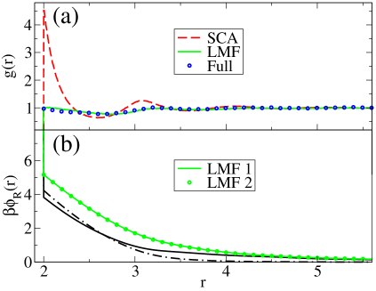
Figure 1: LMF/LR/EXP treatment of the drying transition induced by a hard sphere solute in a LJ fluid for $T=0.85$, $\rho^{B}=0.70$. (a) The RDF around a hard sphere cavity with $R_{c}=2$ for the full LJ fluid, the SCA trial system, and the converged LMF system. (b) Trial fields in the linear regime (solid and dot-dashed curves) and the final self-consistent field (circles and solid line) sim-details .

Strong reduction already is seen for $R_{c}=2$. The circles in Fig. 1a give results of computer simulations sim-details for the radial distribution function (RDF) $g(r;[\phi_{0}])\equiv\rho(r;[\phi_{0}])/\rho^{B}$ induced by the hard sphere solute in the full LJ fluid with bulk density $\rho^{B}$. This exhibits an essentially structureless profile with a contact value of unity. The solid curve in Fig. 1a gives $g_{\rm R}(r;[\phi_{\rm R}])$, the RDF in the mimic system. The excellent agreement between the LMF prediction and the full LJ $g(r;[\phi_{0}])$ shows that LMF theory quantitatively captures the drying effect. This contrasts with the dashed line in Fig. 1a, the density in the truncated system induced by the bare field $\phi_{0}$. The failure of this SCA prediction illustrates the general need in most nonuniform systems for a proper self-consistent solution of the LMF equation.

The self-consistent field $\phi_{\rm R}(r)$ was obtained from solving Eq. (1) using two different trial fields shown in Fig. 1b. Both trial systems are in the linear regime and give the same final result. The solid curve results from a previous trial simulation based on the SCA that used the bare $\phi_{0}(r)$. As Fig. 1a suggests, this represents a very poor initial guess, and the EXP form (3) produced very noisy data, indicating poor overlap between the SCA and final LMF configurations. However Eq. (4) gave much smoother data and its use in the LMF equation gave the solid curve in Fig. 1b as the output field. Using this as a second trial field generates a converged solution of the LMF equation using either Eqs. (4) or (3).

Since $u_{1}$ is slowly-varying, using relatively crude approximations to the asymmetric density in the LMF equation can often give a better trial field than the simple SCA. Thus in Fig. 1b, the dot-dashed trial field was found by approximating the density by a step function that vanishes inside the cavity and equals $\rho^{B}$ outside.

LMF theory proves even more useful Chen et al. (2004); Rodgers and Weeks (2008a) when applied to systems with Coulomb interactions in the presence of an electrostatic potential $\mathcal{V}(\mathbf{r})$ arising from a fixed external charge distribution $\rho^{q}_{\rm ext}(\mathbf{r^{\prime}})$. The basic Coulomb interaction $1/r\equiv v_{0}(r)+v_{1}(r)$ is separated into short- and long-ranged components, where $v_{1}(r)$ is proportional to the electrostatic potential arising from a normalized Gaussian charge distribution with width $\sigma$,

$$v_{1}(r)\equiv\frac{1}{\pi^{3/2}\sigma^{3}}\int e^{-r^{\prime 2}/\sigma^{2}}\frac{1}{\left|\mathbf{r}-\mathbf{r^{\prime}}\right|}\,d\mathbf{r}^{\prime}=\frac{\operatorname{erf}(r/\sigma)}{r}~{}.$$ (6)

An advantage of the Coulomb separation is that $\sigma$ can be chosen specifically in different applications so that condition i) is very well satisfied.

When all charges in the system (both fixed and mobile) are separated using the same $\sigma$ and all other intermolecular interactions remain unchanged, LMF theory then gives a mapping to a Coulomb mimic system where all $1/r$ interactions are replaced by the short-ranged $v_{0}(r)$  and there is a restructured electrostatic potential $\mathcal{V}_{\rm R}$  that satisfies the Coulomb LMF equation

$$\mathcal{V}_{\rm R}(\mathbf{r})=\mathcal{V}_{0}(\mathbf{r})+\int d\mathbf{r}^{\prime}\rho^{q}_{\rm R,tot}(\mathbf{r}^{\prime};[\mathcal{V}_{\rm R}])\,v_{1}(\left|\mathbf{r}-\mathbf{r^{\prime}}\right|)+C.$$ (7)

Here $\mathcal{V}_{0}(\mathbf{r})$ is the short-ranged part of the external potential, given by the convolution of $v_{0}(r)$ with the fixed charge density, and $\rho^{q}_{\rm R,tot}(\mathbf{r}^{\prime};[\mathcal{V}_{\rm R}])$ is the total equilibrium charge density from both fixed and mobile charges. An alternate form of Eq. (7) better relates LMF theory to conventional electrostatics Rodgers and Weeks (2008a). Noting the convolution defining $v_{1}$, we see that the slowly-varying part $\mathcal{V}_{\rm R1}(\mathbf{r})\equiv\mathcal{V}_{\rm R}(\mathbf{r})-\mathcal{V}_{0}(\mathbf{r})$ of the restructured potential in (7) exactly satisfies Poisson’s equation but with a Gaussian-smoothed charge density $\rho^{q\sigma}_{\rm R,tot}$, given by the convolution of $\rho^{q}_{\rm R,tot}$ with the Gaussian in Eq. (6).

We now apply the Coulomb LMF Eq. (7) to the extended simple point charge (SPC/E) model for water Berendsen et al. (1987). As suggested by the SCA, we first consider a Gaussian-truncated (GT) model, where all the $1/r$ interactions from charges in SPC/E water are replaced by $v_{0}(r)$ and we ignore all structural effects from $v_{1}$. Bulk GT water with $\sigma=0.45$ nm gives excellent results for both atom-atom and dipole-angle correlation functions when compared to the full SPC/E model, with Coulomb interactions treated by Ewald sums Rodgers and Weeks (2008a).

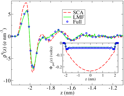
Figure 2: Charge densities for water confined by hydrophobic LJ walls Lee et al. (1984) centered at $z=\pm 2.25$ nm for the SCA (dashed line), mimic system (solid line) and full system (circles). The inset shows the corresponding polarization potentials sim-details .

Moreover, as Fig. 2 shows, when GT water is confined between two hydrophobic LJ walls as defined in Lee et al. (1984), the charge density $\rho^{q}_{0}(z)$ determined by simulations sim-details using bare wall fields with $\mathcal{V}_{0}=0$ seems to capture most qualitative features of the dipole layer, a characteristic property of water near extended hydrophobic interfaces Rodgers and Weeks (2008a); Lee et al. (1984). Only small differences in the peak heights are visible when compared with full SPC/E water, simulated using the slab-corrected Ewald 3D method Yeh and Berkowitz (1999).

Nevertheless, as has long been recognized Feller et al. (1996); Spohr (1997), major errors are seen in the polarization potential felt by a test charge, given by integrating Poisson’s equation:

$$\Phi_{\text{pol}}(z)=-\int_{-L/2}^{z}dz^{\prime}\int_{-L/2}^{z^{\prime}}dz^{\prime\prime}\rho^{q}(z^{\prime\prime}).$$ (8)

As shown in the inset of Fig. 2 for the full SPC/E model, $\Phi_{\text{pol}}$ should reach a plateau in the central bulk region, and GT water fails dramatically in this respect.

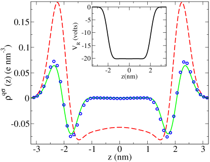
Figure 3: Gaussian-smoothed charge densities with $\sigma=0.45$ nm. Labels are the same as in Fig. 2. The inset gives the effective field ${\cal V}_{\rm R}({\mathbf{r}})$. Note that the bare ${\cal V}({\mathbf{r}})=0$ in this case.

A self-consistent solution of Eq. (7) yields a very accurate charge density that corrects all such failures. The inset in Fig. 3 gives the converged $\mathcal{V}_{\rm R}(z)$. Gaussian smoothing of the bare charge density as dictated by LMF theory averages over the simulation noise and local structure and reveals the much smaller coherent long-wavelength features that control the electrostatics Rodgers and Weeks (2008a). The smoothed charge density quickly decays to a neutral bulk in Fig. 3 for both SPC/E water and LMF theory, while a true bulk never forms in GT water, causing the very poor polarization potential in Fig. 2.

These results highlight the advantages of the new LR-LMF method. It reduced the simulation time by more than an order of magnitude compared to use of the standard iteration method Rodgers and Weeks (2008a) or to use of the slab-corrected Ewald 3D method Yeh and Berkowitz (1999). When using the standard iteration method, it proved very difficult to distinguish between equilibrium charge density fluctuations, present for any given field, and the desired changes in the charge density as the iteration proceeded to self-consistency. To obtain convergence, earlier workers had to use a large value of $\sigma=0.6$ nm and the charge density at each iteration was taken as the average over a set of 10 parallel simulations with different initial conditions Rodgers and Weeks (2008a).

In contrast, the results in Figs. 2 and 3 were obtained from only two very short trial simulations sim-details , starting first with the SCA $\mathcal{V}_{0}=0$, and using the smaller bulk $\sigma=4.5$ nm. As before, the EXP form (3) was very noisy when used with SCA configurations, but the LR form (4) was much better behaved. It generated a second trial field in the linear regime that was virtually identical to the final self-consistent field shown in the inset of Fig. (3). The remaining effects of equilibrium fluctuations in the mimic system show up as small variations (about the size of the circle symbol) in the bulk value of the polarization potential in Fig. 2 or the heights of the charge density peaks in Fig. 3. As shown in the supplementary material, excellent results have also been obtained for ion pairing in ionic solution models using the LR-LMF method sim-details .

Reaction field (RF) truncations of Coulomb interactions have recently been used in massively-parallel simulations of biological systems to permit much faster simulations Schulz2009 . LR-LMF theory may provide a promising linear-scaling alternative in which the effective field corrects known problems like those illustrated in Fig. 2 arising from simple RF or SCA truncations. More generally, we believe the efficient solutions generated by the LR-LMF method establish the full power of the basic mean field picture for both quantitative and qualitative analysis of a wide range of electrostatic and dielectric phenomena in nonuniform liquids.

This work was supported by the National Science Foundation (grants CHE0628178 and CHE0848574). We are grateful to Gerhard Hummer, Chris Jarzynski, and Jocelyn Rodgers for very helpful remarks.

References

- (1) See, e.g., L.P. Kadanoff, Statistical Physics (World Scientific, Singapore, 2000), pp. 209-246.
- Weeks et al. (1998) J.D. Weeks, K. Katsov, and K. Vollmayr, Phys. Rev. Lett. 81, 4400 (1998); K. Katsov and J. D. Weeks, J. Phys. Chem. B 105, 6738 (2001).
- Weeks (2002) J.D. Weeks, Ann. Rev. Phys. Chem. 53, 533 (2002).
- Chen et al. (2004) Y.-G. Chen, C. Kaur, and J.D. Weeks, J. Phys. Chem. B 108, 19874 (2004); J. M. Rodgers, C. Kaur, Y.-G. Chen and J. D. Weeks, Phys. Rev. Lett. 97, 097801 (2006).
- Rodgers and Weeks (2008a) J. M. Rodgers and J. D. Weeks, Proc. Nat. Acad. Sci. USA 105, 19136 (2008a); J. M. Rodgers and J. D. Weeks, J. Phys.: Cond. Matt. 20, 494206 (2008b).
- (6) R. Schulz, B. Lindner, L. Petridis, and J.C. Smith, J. Chem. Theory Comput. 5, 2798 (2009).
- Weeks et al. (1971) J.D. Weeks, D. Chandler, and H.C. Andersen, J. Chem. Phys. 54, 5237 (1971).
- (8) A general field can be used in Eq. (1) as well.
- Chipot and Pohorille (2007) See, e.g., Free Energy Calculations: Theory and Application in Chemistry and Biology, edited by C. Chipot and A. Pohorille (Springer, Berlin, 2007).
- Huang and Chandler (2000) D. M. Huang and D. Chandler, Phys. Rev. E 61, 1501 (2000).
- (11) See EPAPS supplementary material at [URL to be inserted] for simulation details.
- Berendsen et al. (1987) H.J.C. Berendsen, J.R. Grigera, and T.P. Straatsma, J. Phys. Chem. 91, 6269 (1987).
- Lee et al. (1984) C.Y. Lee, J.A. McCammon, and P.J. Rossky, J. Chem. Phys. 80, 4448 (1984).
- Yeh and Berkowitz (1999) I.-C. Yeh and M. L. Berkowitz, J. Chem. Phys. 111, 3155 (1999).
- Feller et al. (1996) S. E. Feller, R. W. Pastor, A. Rojnuckarin, S. Bogusz, and B. R. Brooks, J. Phys. Chem. 100, 17011 (1996).
- Spohr (1997) E. Spohr, J Chem Phys 107, 6342 (1997).