A discontinuous Galerkin method for the Vlasov-Poisson system

Abstract

A discontinuous Galerkin method for approximating the Vlasov-Poisson system of equations describing the time evolution of a collisionless plasma is proposed. The method is mass conservative and, in the case that piecewise constant functions are used as a basis, the method preserves the positivity of the electron distribution function and weakly enforces continuity of the electric field through mesh interfaces and boundary conditions. The performance of the method is investigated by computing several examples and error estimates associated system’s approximation are stated. In particular, computed results are benchmarked against established theoretical results for linear advection and the phenomenon of linear Landau damping for both the Maxwell and Lorentz distributions. Moreover, two nonlinear problems are considered: nonlinear Landau damping and a version of the two-stream instability are computed. For the latter, fine scale details of the resulting long-time BGK-like state are presented. Conservation laws are examined and various comparisons to theory are made. The results obtained demonstrate that the discontinuous Galerkin method is a viable option for integrating the Vlasov-Poisson system.

1 Introduction

The single species Vlasov-Poisson system is a nonlinear kinetic system that models time evolution of a collisionless plasma consisting of electrons and a uniform background of fixed ions under the effects of a self-consistent electrostatic field and possibly an externally supplied field. The Vlasov equation models the transport of the electrons that are coupled to the electrostatic potential through Poisson’s equation.

The unknown electron distribution function, a phase space density, is denoted by $f=f(x,v,t),$ where the independent variables $x,v,t$ are position, velocity, and time, respectively. For a given $t$, the quantity $f(x,v,t)\,dxdv$ denotes the number of electrons contained in the infinitesimal phase space volume element $dxdv$ centered about $(x,v)$ at time $t$. Upon a proper renormalization, $f$ can be interpreted as a probability distribution function for the electrons over the phase space.

The Vlasov-Poisson system has solutions that can exhibit a variety of dynamical phenomena [69, 7, 44]. One of the most well-known effects is filamentation or ‘phase mixing’ as it is sometimes called, which occurs when different characteristics surfaces associated to the nonlinear transport (Vlasov) equation wrap in the phase space. This effect results in stiff gradients, since $f$ generally takes on disparate values along different characteristics.

Related to filamentation is the interesting phenomenon of Landau damping [42]: electrostatic disturbances can be interpreted as the interaction between plasma waves and electrons with a resulting net energy transfer from the wave to electrons leading to an exponential collisionless damping of the electric field modes in time. Because of such phenomena, the Vlasov-Poisson equation can be challenging to simulate numerically.

Existing numerical techniques for solving the Vlasov-Poisson system can be divided into two groups: (i) those that approximate the system in the phase space directly and (ii) those that transform the system into a different coordinate space. The numerical approaches that treat the phase space directly do not, however, usually involve discretizing the Vlasov equation. Rather most of these methods take advantage of the characteristic structure of the Vlasov equation, which implies that the plasma particles evolve along trajectories that satisfy a given set of ordinary differential equations. The most widely used particle scheme is the Particle-in-Cell (PIC) method [9, 38, 27], which represents ensembles micro-particles as a finite number of macro-particles. Each macro-particle is then assumed to evolve along a characteristic trajectory, where the electric field defining the trajectory is computed via any standard scheme. The PIC method seems to give reasonable results in cases where the tail of the distribution is negligible and a large number of particles is not necessary. Otherwise, the method suffers from numerical noise that is proportional to $1/\sqrt{n},$ where $n$ is the number of particles.

Other methods based on the discretization of the phase space have also been proposed. In [11], an operator splitting method was introduced and shown to be both efficient and accurate for solving a wide range of problems. A continuous finite element method was developed in [72, 73] and was shown to achieve results similar to those obtained in [11]. A positive and mass conservative scheme was employed in [33] to solve both linear and nonlinear damping problems in one- and two-dimensional physical space. This method is defined at a given time step by first building a piecewise constant approximation over a mesh of the phase space using the approximation obtained from the previous time step and two correction terms whose values are found by solving two fixed point problems. The piecewise approximation is then used in conjunction with a slope limiter to reconstruct a local polynomial approximation of $f$ for each cell in the mesh.

Transform methods based on Fourier or Hermite series have also been used, e.g. in [36, 3, 29] and more recently in [31]. In [40, 41], the phase space was transformed using a Fourier transform and a splitting method was employed to advance the approximation in time. This method also included a filamentation filtering step for the purpose of smoothening the filaments. The numerical results obtained using this method seem reasonable only for problems in which filamentation is not a dominant effect, where perhaps the nonlinearity either slows down or prevents the onset of filamentation. However, this method may be inadequate for problems where the physics of interest depends upon the filamentary nature of the distribution, such as is the case for Landau damping.

The objective of this paper is to propose a coupled Upwind Penalty Galerkin (UPG) method for the approximation of the Vlasov-Poisson system and to evaluate its numerical efficacy. Our UPG method gives a unified approach for approximating both the hyperbolic and elliptic parts of the Vlasov-Poisson system. Specifically, the Vlasov equation is discretized using the standard Upwind Galerkin (UG) scheme for conservation laws [24, 23, 22] and the Poisson equation is discretized using one of the three Discontinuous Galerkin (DG) interior penalty available schemes [70, 59, 63]. Stability and convergence estimates for the UPG method were presented in [37] for the six-dimensional phase space In the same reference, the method was shown to be both locally and globally mass conservative.

More specifically, the semi-discrete UPG approximation $f_{h}$ to the electron distribution function is defined to be the solution of a first-order, nonlinear, ordinary differential equation (ODE) system. Moreover, it has been shown that the method preserves positivity of $f_{h}$ when piecewise constants basis functions are used to approximate the solution to the Vlasov-Poisson system.

In this manuscript we show the numerical efficacy of the DG method by performing accuracy, convergence, and conservation tests on computed UPG approximate solutions to a variety of linear and nonlinear problems where sufficiently data or information of the true nonlinear solutions has been established. The computed results for these problems are benchmarked against known theoretical results and are compared to results obtained using established methods.

For computing plasma problems the UPG method offers several advantages. In particular, the local nature of the method facilitates adaptive mesh refinements with easy adaptation to parallelization techniques. By taking advantage of these benefits, regions of the phase space where the electron distribution experiences strong filamentation or boundary layer effects can be resolved by local mesh refinements. The discontinuous nature of the method also helps to resolve the stiff gradients associated with filamentation, since requiring the approximation to be continuous in these cases can be too restrictive and typically lead to excessive numerical diffusion and oscillatory behavior. Due to the fact that the method imposes boundary conditions weakly, a variety of boundary conditions can easily be accommodated.

Recently, an alternative DG formulation for the Boltzmann-Poisson system was introduced in [12, 13, 14, 15, 16] for simulations of hot electron transport for one and two space dimensional nanometer scale devices, where kinetic corrections are known to be very significant. In [20] a DG scheme was constructed for the Vlasov-Boltzmann equation by means of a maximum principle satisfying a limiter for conservation laws [74, 75], and it was shown to be high order accurate and positivity-preserving, not only for piecewise constant basis functions but also for higher order polynomial approximations. Consequently a new approximation of the Vlasov system based on a UPG scheme for higher order polynomial basis functions is currently being developed and tested [18, 17]. Thus, the DG method is well-suited to approximate a range of plasmas spanning from the collisionless to the highly collisional regimes.

For completeness of this introduction we include some historical remarks regarding DG methods. The initial development of these numerical approximating schemes for hyperbolic and elliptic equations occurred independently, but nearly simultaneously. In 1973, the first DG scheme for linear hyperbolic equations was introduced by Reed and Hill for approximating a neutron transport equation [57]. This work was followed by Lesaint and Raviart [43] in 1974, where a priori error estimates were proved for the DG method applied to two-dimensional, linear hyperbolic problems. The DG schemes for hyperbolic problems were further studied in the series of papers [24, 23, 22], which culminated in the introduction of the local discontinuous Galerkin (LDG) method [25]. The generality of the LDG method was further extended to the multidimensional setting under more relaxed assumptions on the data in [21]. One of the first DG schemes for approximating the solutions to second-order elliptic equations was introduced in 1971 by Nitsche [55] where Dirichlet boundary conditions were enforced weakly rather than strongly through the use of a penalty term. Shortly thereafter, applications of the penalty method to Laplace’s equation were proposed by Babuška et al.  in [4, 5, 6].

The use of penalty terms across interior faces as a means of enforcing continuity among adjacent elements was introduced in [70] and [71] using a symmetric interior penalty Galerkin (SIPG) finite element method. A non-symmetric interior penalty method (NIPG) similar to the SIPG method was proposed and analyzed in [59]. The incomplete interior penalty method (IIPG) was introduced in [63, 28, 64] and is very similar to the SIPG and NIPG methods.

The outline of this paper is as follows. In Section 2, we describe the Vlasov-Poisson system and give a brief discussion of Landau damping. In Section 3, the UPG method for the approximation of the Vlasov-Poisson system is derived and the error estimates associated to the approximation of the system are stated. In Section 4, several numerical simulation results are presented and analyzed, including a study of the free streaming operator (simple advection), Landau damping for Maxwellian and Lorenztian equilibria, strong nonlinear Landau damping and a careful study of a symmetric two-stream instability, all for the case of repulsive potential forces. In Section 5, we comment on the efficiency of the UPG method, draw some conclusions, and remark on future work. Finally, an Appendix dedicated to the analysis of dispersion relations for the Lorentzian and two-stream equilibria is included.

2 The Vlasov-Poisson System

The Vlasov-Poisson system considered in this work has been scaled by the usual characteristic time and length scales, i.e., time is scaled by the inverse plasma frequency $\omega^{-1}_{p}$, length by the Debye length $\lambda_{D}$, and velocity accordingly by a thermal velocity $v_{th}=\omega_{p}\lambda_{D}$.

Using this nondimensionalization, the Vlasov-Poisson problem is as follows: For the divergence free vector in $(x,v)$ phase space

$$\alpha(x,v,t)=(v,-E(v,t))\,\qquad\mathrm{for}\ (x,v,t)\in\Omega\times[0,T]\,,$$ (1)

find the electron distribution function $f(x,v,t)$ and the electric field $E(x,t)$ with corresponding electrostatic potential $\Phi(x,t)$ such that, for fixed $T>0$,

$$0 \ =\ \partial_{t}f+\mathrm{div}(\alpha\,f)\ =\ \partial_{t}f+v\cdot\nabla_{x}f-E\cdot\nabla_{v}f\,, \ \text{in}\ \Omega\times(0,T]\,,\ \,$$ (2a)

$$E \ =-\nabla_{x}\Phi\,;\ \ \ -\Delta_{x}\Phi\ =\ 1-\int_{\mathbb{R}^{n}}\,f\,dv\,,\ \ \text{in}\ \Omega_{x}\times(0,T]\,,$$ (2b)

subject to an initial condition on $f$ and boundary conditions on $f$ and $\Phi.$ The domain of definition of the initial boundary value problem $\Omega:=\Omega_{x}\times\mathbb{R}^{n}$, where the physical domain $\Omega_{x}\subset\mathbb{R}^{n}$ can either be bounded or all of $\mathbb{R}^{n}$ with $n=1,2,3$. The boundary condition given for $f$ depends on $\Omega_{x}.$ If $\Omega_{x}=\mathbb{R}^{n},$ then the condition $f\rightarrow 0$ must be enforced both as $|x|\rightarrow\infty$ and as $|v|\rightarrow\infty.$ If $\Omega_{x}$ is bounded, then a condition must be imposed on $f$ along the inflow boundary $\Gamma_{{}_{I}},$ defined by

$$\Gamma_{{}_{I}}\ =\ \{(x,v)\in\partial\Omega_{x}\times\mathbb{R}^{n}\,|\,v\cdot\nu_{{}_{x}}<0\}\,,$$ (3)

with $\nu_{{}_{x}}$ being the unit outward normal vector to $\partial\Omega_{x}.$ Often $f_{{}_{I}}$ is given in some parts of the boundary and may be periodic in other parts of the boundary region $\Gamma_{{}_{I}}$. In this manuscript we assume periodic boundary conditions in space and the decaying boundary condition in velocity.

The Poisson equation must also be endowed with spatial boundary conditions, either Dirichlet, Neumann, Robin, or periodic, on different disjoint regions of the boundary $\partial\Omega_{x}$. We denote the Dirichlet portion of the boundary by $\partial\Omega_{x,D}$. If the measure of the Dirichlet boundary is zero, i.e. $|\partial\Omega_{x,D}|=0$, and one has homogeneous or periodic boundary conditions such that $\int_{\partial\Omega_{x}}\nabla\Phi\cdot\nu_{x}=0$, then in order to maintain a well-posed problem that keeps the existence and uniqueness of the corresponding Poisson boundary value problem, one needs to add to the solution space the compatibility (neutrality) condition $\int_{\Omega_{x}}(1-\int_{\mathbb{R}^{n}}\,f\,dv\,)dx=0$, or equivalently $\int_{\Omega_{x}}\int_{\mathbb{R}^{n}}\,f\,dx\,dv=|\Omega_{x}|$ on each connected component of the spatial domain $\Omega$.

Macroscopic fluid quantities of interest are easily computed from $f$. The electron density $\rho=\rho(x,t)$, current density $j=j(x,t)$, kinetic energy density $\mathcal{E}_{k}(x,t)$ and electrostatic energy density $\mathcal{E}_{e}(x,t)$ are defined by

$$\rho(x,t)\ =\ \int\limits_{\mathbb{R}^{n}}f(x,v,t)\,dv\,,$$ (4)

$$j(x,t)\ =\ \int\limits_{\mathbb{R}^{n}}vf(x,v,t)\,dv\,,$$ (5)

$$\mathcal{E}_{k}(x,t)\ =\ \frac{1}{2}\,\int\limits_{\mathbb{R}^{n}}|v|^{2}f(x,v,t)\,dv\,,$$ (6)

$$\mathcal{E}_{e}(x,t)\ =\ \frac{1}{2}\,|E(x,t)|^{2}\,.$$ (7)

These quantities satisfy a number of respective conservation laws (see e.g. [58]). In particular, it is well-known that the Vlasov-Poisson system conserves total particle number, momentum, energy, and the Casimir invariants, which are given, respectively, by

$$N\ =\ \int_{\Omega_{x}\times{\mathbb{R}^{n}}}f(x,v,t)\,dx\,dv=\int_{\Omega_{x}}\,\rho(x,t)\,dx\,,$$ (8)

$$P\ =\ \int_{\Omega_{x}\times{\mathbb{R}^{n}}}vf(x,v,t)\,dx\,dv=\int_{\Omega_{x}}j(x,t)\,dx\,,$$ (9)

$$H\ =\ \frac{1}{2}\int_{\Omega_{x}\times{\mathbb{R}^{n}}}|v|^{2}f(x,v,t)\,dx\,dv+\frac{1}{2}\,\int_{\Omega_{x}}|E(x,t)|^{2}\,dx$$ (10)

$${\ }\ \hskip 18.06749pt=\int_{\Omega_{x}}\big{(}\mathcal{E}_{k}(x,t)+\mathcal{E}_{e}(x,t)\big{)}\,dx\,,$$

$$C\ =\ \int_{\Omega_{x}\times{\mathbb{R}^{n}}}\,\mathcal{C}(f)\,dx\,dv\,,$$ (11)

The notation $\mathcal{C}(f)$ in (11) refers to an arbitrary function of $f$ and includes the ‘enstrophy’ when $\mathcal{C}(f)=f^{2}$, entropy when $\mathcal{C}(f)=-f\ln f$, or particle number, as in (8), when $\mathcal{C}(f)=f$. We will check the invariance of these quantities in our nonlinear computations, particularly in Section 4.2.2.

Interesting properties of the Vlasov-Poisson system result by considering a linear perturbation $\delta f(x,v,t)$ to an equilibrium distribution $f_{eq}(v)$ over the 2D-phase space $[0,L]\times(-\infty,\infty),\ L>0.$ Specifically, suppose that $f=f_{eq}+\delta f$, where $f_{eq}$ is a given equilibrium probability distribution, $\delta f$ and $\Phi$ are $L$-periodic in $x$, and the initial average value of $\delta f$ over $\Omega$ is zero. Equations (2a)-(2b) imply that $\delta f$ satisfies

$$\partial_{t}(\delta f)+v(\delta f)_{x}-E(\delta f)_{v} \ =\ Ef_{eq}^{\prime} [0,L]\times(-\infty,\infty)\times(0,T]\,,$$ (12a)

$$E \ =\ -\Phi_{x} [0,L]\times(0,T]\,,$$ (12b)

$$\Phi_{xx} \ =\ \int_{\mathbb{R}^{n}}\,\delta f\,dv [0,L]\times(0,T]\,.$$ (12c)

Supposing $|E(\delta f)_{v}|<<1$ and dropping this term from (12a) leads to

$$\partial_{t}(\delta f)+v(\delta f)_{x} \ =\ Ef_{eq}^{\prime} [0,L]\times(-\infty,\infty)\times(0,T]\,,$$ (13a)

$$E \ =\ -\Phi_{x} [0,L]\times(0,T]\,,$$ (13b)

$$\Phi_{xx} \ =\ \int_{\mathbb{R}^{n}}\,\delta f\,dv [0,L]\times(0,T]\,.$$ (13c)

The linear system of (13a)-(13c) was analyzed by using the Laplace transform in the famous paper of Landau [42], by expansion in terms of continuum eigenfunctions in [69], and by a tailored integral transform introduced in [51, 52]. Landau showed that an electric field mode $E_{k}(\omega,t)$ decays exponentially in the long-time limit, which we investigate in Section 4.1.2 for two well-known equilibria: the Maxwellian

$$f_{M}=(2\pi T)^{-n/2}\,e^{-v^{2}/2T}\,,$$ (14)

and the Lorentzian,

$$f_{L}(v)=\ \frac{1}{\pi}\,\frac{\gamma}{v^{2}+\gamma^{2}}\,.$$ (15)

3 Method Formulation

In this section, we derive the UPG method for the Vlasov-Poisson system. The derivation proceeds by first discretizing the Vlasov equation using the standard UG discretization for transport equations [21]. Here it is assumed that the electric field is given and hence the divergence-free flow field $\alpha(x,v,t)=(v,-E(x,t))$, defined in (1) for the Vlasov equation (2a), is known. Afterwards, the DG discretization for the Poisson equation is considered.

It is assumed that any mesh for the phase space, where by mesh we mean a partitioning of the phase space into convex sets called elements, is the Cartesian cross product of a mesh for the physical domain and a mesh for the velocity domain. Under this assumption, the physical and velocity domains can be independently refined. Given a mesh for the phase space, the UG method then defines an approximate solution to the true Vlasov solution in such a way that at any given time the approximate solution restricted to each element of the mesh is a polynomial function. However, the approximate solution is not required to be continuous across the intersections of any two adjacent elements, so it is a piecewise defined polynomial function with respect to the mesh at any given time.

In order to compute the approximation to the electrostatic potential from Poisson’s equation (2b), for a given distribution function, one may use one of three interior penalty methods that weakly enforce both approximate continuity across the interior mesh faces and Dirichlet boundary regions. These three alternative methods, symmetric interior penalty Galerkin (SIPG) [70, 71], non-symmetric interior penalty Galerkin (NIPG) [59], and incomplete interior penalty Galerkin (IIPG) [63, 64] are discussed in detail and a priori error estimates for each of them are given in the respective references. The only difference among the three methods is in the value of one specific parameter that arises in the weak formulation that is common to each of them. Thus, for a given space charge function, each penalty Galerkin method defines a piecewise polynomial approximation of the true solution to the Poisson equation using a mesh in the spatial domain.

The spatial domain mesh used in the discretization of Poisson’s equation is required to be the same as that used in the UG discretization of the Vlasov equation. This requirement is a practical one, both in terms of analysis and implementation. However, the polynomial degree of the potential approximation on a given element of the spatial mesh is not required to equal the degree, with respect to $x$, of the polynomial approximation of the distribution $f$.

Thus, the UPG method of approximation to the Vlasov-Poisson system is defined by coupling together the UG method of approximation to the Vlasov equation with interior penalty methods of approximation to the Poisson equation. This nonlinear semi-discrete approximation results in a first-order nonlinear ODE system, the solution of which determines the approximation $f_{h}$ of $f$. The resulting ODE system is readily solved using an explicit conservative time-integrator such as the Runge-Kutta method. Moreover, in the process of computing $f_{h}$, both the approximation $E_{h}$ of the electric field $E$ and the approximation $\Phi_{h}$ of the potential $\Phi$ are computed by one of the penalty methods for the elliptic equation.

3.1 Preliminaries

We assume the computational domain in velocity space is a bounded set $\Omega_{v}$ and that the approximate solution to $f(x,v,t)$ is assumed to vanish in $\partial\Omega_{v}$. It is then, implicitly for our simulation, assumed that the velocity support of the approximation to the true solution $f$ of the Vlasov-Poisson system is contained in $\Omega_{v}$ for all times. This is a reasonable assumption for problems with spatial periodic boundary conditions, as it is expected that most of the density associated with the approximation to $f$ will be contained in a sufficiently large fixed set $\Omega_{v}$. The error due to this assumption only depends on the density of the true solution $f$ computed on the complement of $\Omega_{v}$ in $\mathbb{R}^{n}$.

Further, the conservative nature of the transport equation (2a) with the space dependent divergence-free flow field $\alpha$, motivates us to choose the computational scheme as follows:

Let $\{\mathcal{T}_{h_{x}}\}_{h_{x}>0}$ be a sequence of successively refined meshes of the bounded domain $\Omega_{x}\subset\mathbb{R}^{n}$ and let $\{\mathcal{T}_{h_{v}}\}_{h_{v}>0}$ be a sequence of successively refined meshes of the bounded domain $\Omega_{v}\subset\mathbb{R}^{n}$, where $n=1,2,3.$ Given the meshes $\mathcal{T}_{h_{x}}=\{K_{j_{x}}\}_{j_{x}=1}^{N_{h_{x}}}$ and $\mathcal{T}_{h_{v}}=\{K_{j_{v}}\}_{j_{v}=1}^{N_{h_{v}}}$, the elements $K_{j_{x}}$ and $K_{j_{v}}$ comprising each of the respective meshes are sets of the following types: intervals, if $n=1$; triangles or quadrilaterals, if $n=2$; and tetrahedra, prisms or hexahedra, if $n=3$. The corresponding spatial refinement level $h_{x}$ and velocity refinement level $h_{v}$ are defined by $h_{x}=\max_{j_{x}}\,\{\mathrm{diam}(K_{j_{x}})\}$ and $h_{v}=\max_{j_{v}}\,\{\mathrm{diam}(K_{j_{v}})\}$, respectively.

A sequence of successively refined meshes $\{\mathcal{T}_{h}\}_{h>0}$ of the, now, computational domain $\Omega=\Omega_{x}\times\Omega_{v}$ is generated by defining each mesh $\mathcal{T}_{h}=\{K_{j}\}_{j=1}^{N_{h}}$ to be $\mathcal{T}_{h}=\mathcal{T}_{h_{x}}\times\mathcal{T}_{h_{v}},$ where the refinement level is $h=(h_{x},h_{v})$. Thus, for any given element $K_{j}\in\mathcal{T}_{h}$ there exists a unique pair of elements $K_{j_{x}}\in\mathcal{T}_{h_{x}}$ and $K_{j_{x}}\in\mathcal{T}_{h_{x}}$ such that $K_{j}=K_{j_{v}}\times K_{j_{v}}$, which is equivalent to the existence of an invertible mapping from $j\in\{1,\ldots,N_{h}\}$ to $(j_{x},j_{v})\in\{1,\ldots,N_{h_{x}}\}\times\{1,\ldots,N_{h_{v}}\}$, where $N_{h}=N_{h_{x}}N_{h_{v}}$.

The derivation of the following UPG method requires the use of the broken Sobolev space $H^{s}\{\mathcal{T}_{h}\}$, $s>1/2$, which is defined as follows:

$$H^{s}\{\mathcal{T}_{h}\}\ =\ \{\,w\in L^{2}(\Omega)\ |\ w_{{}_{|K_{j}}}\in H^{s}\{K_{j}\},\ \forall\,K_{j}\in\mathcal{T}_{h}\,\}\,,$$ (16)

i.e., $H^{s}\{\mathcal{T}_{h}\}$ is the space of those functions that have elementwise weak derivatives up to, and including, the order $s$. Then for nonnegative integers $r_{x}$ and $r_{v}$, the discontinuous approximation space $D^{r_{x},r_{v}}(\mathcal{T}_{h})\subset H^{s}\{\mathcal{T}_{h}\}$ is given by

$$D^{r_{x},r_{v}}(\mathcal{T}_{h})\ =\ \{\,w\in H^{s}\{\mathcal{T}_{h}\}\ |\ w_{{}_{|K_{j}}}\in\mathbb{Q}^{r_{x}}\{K_{j_{x}}\}\times\mathbb{Q}^{r_{v}}\{K_{j_{v}}\},\ \forall\,K_{j}\in\mathcal{T}_{h}\,\}\,,$$ (17)

where $\mathbb{Q}^{r}(K)$ denotes the space of polynomials on a set $K$ with degree less than or equal to $r$ in each variable. Thus, $\mathbb{P}^{r}(K)\subset\mathbb{Q}^{r}(K)$, where $\mathbb{P}^{r}(K)$ denotes the space of polynomials satisfying that the sum of the degrees of all the variables is less than or equal to $r$.

The choice of $\mathbb{Q}^{r}(K)$ for basis functions is suitable for Cartesian meshes in both $x$-space and $v$-space, respectively, where trace and inverse inequalities that are derived by mapping to the reference element in the approximating framework are possible, as first introduced in [37].

However, one may use triangles in two-dimensions, and prisms or hexahedra in three-dimensions, for both $x$-space and $v$-space, for which the natural choice of polynomial space would be $\mathbb{P}^{r_{x}}\{K_{j_{x}}\}\times\mathbb{P}^{r_{v}}\{K_{j_{v}}\}$. We point out that these selections of approximating spaces is consistent with the divergence free, linear, and conservation form of the Vlasov equation, and the fact that the choice of the mesh associated with the computational domain $\Omega=\Omega_{x}\times\Omega_{v}$ is a set of product mesh elements $K_{j}=K_{j_{v}}\times K_{j_{v}}$, for $j\in\{1,\ldots,N_{h}\}$, $(j_{x},j_{v})\in\{1,\ldots,N_{h_{x}}\}\times\{1,\ldots,N_{h_{v}}\}$ and $N_{h}=N_{h_{x}}N_{h_{v}}$. Such is clearly preserved by the Vlasov flow and the corresponding approximation results for $\mathbb{P}^{r}(K)$ will be valid. This choice may be preferable in higher dimensions since the number of degrees of freedom of the basis functions in $\mathbb{P}^{r}(K)$ is $rn+1$, while for $\mathbb{Q}^{r}(K)$ is $(r+1)^{n}$, for $n$-dimensional calculations.

The discontinuous nature of the space $H^{s}\{\mathcal{T}_{h}\}$ needs the introduction of mesh faces. If $K_{j}$ is a boundary element, then $F_{k}=\partial K_{j}\cap\partial\Omega$ is called a boundary mesh face. If $K_{1}$ and $K_{2}$ are two intersecting elements whose common intersection lies in the interior of $\Omega$, then $F_{k}=\partial K_{1}\cap\partial K_{2}$ is said to be an interior mesh face. The set of all mesh faces is denoted by $\mathcal{F}_{h}=\{F_{1},\ldots,F_{P_{h}},F_{P_{h}+1},\ldots,F_{M_{h}}\}$, where $F_{k}$ is an interior face if $1\leq k\leq P_{h}$ and a boundary face if $P_{h}+1\leq k\leq M_{h}$. Each face $F_{k}\in\mathcal{F}_{h}$ is associated with a unit normal vector $\nu_{k}$. For $k>P_{h}$, $\nu_{k}$ is chosen to be the outward unit normal to $\partial\Omega$. For $1\leq k\leq P_{h}$, we fix $\nu_{k}$ to be one of the two unit normal vectors to $F_{k}.$ For every interior face $F_{k},$ the elements $K_{1}$ and $K_{2}$ will always be used to denote the two unique elements such that $F_{k}=K_{1}\cap K_{2}.$ Moreover, it is always assumed that $K_{1}$ satisfies $\nu_{{}_{K_{1}}}=\nu_{k}$ on $F_{k}$, where $\nu_{{}_{K_{1}}}$ denotes the outward unit normal to $\partial K_{1}.$ Then $\nu_{{}_{K_{2}}}=-\nu_{k}$ on $F_{k}$.

The fact that each mesh $\mathcal{T}_{h}$ is the product of a spatial mesh $\mathcal{T}_{h_{x}}$ and a velocity mesh $\mathcal{T}_{h_{v}}$ gives a specific structure to the boundaries of the elements and to the set of mesh faces $\mathcal{F}_{h}$. It follows that for $K_{j}=K_{j_{x}}\times K_{j_{v}}$ we have $\partial K_{j}=(\partial K_{j_{x}}\times K_{j_{v}})\cup(K_{j_{x}}\times\partial K_{j_{v}})$. We denote the set of mesh faces for $\mathcal{T}_{h_{x}}$ and $\mathcal{T}_{h_{v}}$ by $\mathcal{F}_{h_{x}}=\{F_{1}^{x},\ldots,F_{P_{h_{x}}}^{x},F_{P_{h_{x}}+1}^{x},\ldots,F_{M_{h_{x}}}^{x}\}$ and $\mathcal{F}_{h_{v}}=\{F_{1}^{v},\ldots,F_{P_{h_{v}}}^{v},F_{P_{h_{v}}+1}^{v},\ldots,F_{M_{h_{v}}}^{v}\}$, respectively, where $F_{k_{x}}^{x}$ is an interior face if $1\leq k_{x}\leq P_{h_{x}}$ and a boundary face if $P_{h_{x}}+1\leq k_{x}\leq M_{h_{x}}$, and $F_{k_{v}}^{v}$ is an interior face if $1\leq k_{v}\leq P_{h_{v}}$ and a boundary face if $P_{h_{v}}+1\leq k_{v}\leq M_{h_{v}}$. Then, given any arbitrary $F_{k}\in\mathcal{F}_{h}$, either there exist an $F_{k_{x}}^{x}\in\mathcal{F}_{h_{x}}$ and a $K_{j_{v}}\in\mathcal{T}_{h_{v}}$ such that $F_{k}=F_{k_{x}}^{x}\cup K_{j_{v}}$ or there exist a $K_{j_{x}}\in\mathcal{T}_{h_{x}}$ and an $F_{k_{v}}^{v}\in\mathcal{F}_{h_{v}}$ such that $F_{k}=K_{j_{x}}\cup F_{k_{v}}^{v}$.

When considering functions in $H^{s}\{\mathcal{T}_{h}\}$, we use the usual average and jump operators, respectively, defined for $w\in H^{s}\{\mathcal{T}_{h}\}$ along an interior face $F_{k}$ by

$$\overline{w}\ =\ \frac{1}{2}\,\left(\,(w_{|K_{1}})_{|F_{k}}\ +\ (w_{|K_{2}})_{|F_{k}}\,\right)\,,\qquad[\,w\,]\ =\ (w_{|K_{1}})_{|F_{k}}\ -\ (w_{|K_{2}})_{|F_{k}}\,.$$ (18)

The above definitions are also valid for vector-valued functions $w\in[H^{s}\{\mathcal{T}_{h}\}]^{2n}$, in which case it follows that $[w]\cdot\nu_{k}=(w_{|K_{1}})_{|F_{k}}\cdot\nu_{K_{1}}+(w_{|K_{2}})_{|F_{k}}\cdot\nu_{K_{2}}$.

3.2 Upwind Galerkin Approximation of the Vlasov Equation

Here we describe the UG scheme for the Vlasov equation in full generality for a $2n$-dimensional ($n=1,2$ or $3$) phase space with inflow boundary conditions and piecewise polynomials of arbitrary degree approximating $f$. The simpler derivation of the method for a two-dimensional phase space with periodic boundary conditions in $x$ and a piecewise constant approximation to $f$ is given explicitly in Section 3.5, since this method was used for the numerics of Section 4. Note, for this simpler version the derivation does not require use of the set of mesh faces $\mathcal{F}_{h}$.

For a given time $T>0$ and data trio $(\alpha,f_{{}_{0}},f_{{}_{I}})$, the Vlasov equation along with the corresponding initial and boundary conditions are

$$\partial_{t}f+\alpha\cdot\nabla f\ =\ 0\qquad \Omega\times(0,T]\,,$$ (19a)

$$f(t=0)\ =\ f_{{}_{0}}\qquad \Omega\,,$$ (19b)

$$f\ =\ f_{{}_{I}}\qquad \Gamma_{{}_{I}}\times(0,T]\,,$$ (19c)

where $\alpha=(v,-E)\in\mathbb{R}^{2n}$, $E\in\mathbb{R}^{n}$ is assumed given, $\nabla=(\nabla_{x},\nabla_{v})$, and $\Omega=\Omega_{x}\times\Omega_{v}$. It is assumed that $\Omega_{x}=\Pi_{i=1}^{n}[0,X_{i}]$ and $\Omega_{v}=[-V_{c},V_{c}]^{n},$ where $X_{1},\ldots,X_{n},V_{c}>0$ are fixed. Following (3), we also define (keeping the same notation without loss of generality) the computational inflow boundary $\Gamma_{{}_{I}}$, associated with the computational domain $\Omega$, by

$$\Gamma_{{}_{I}}\ =\ \{(x,v)\in\partial\Omega\ |\ \alpha\cdot\nu<0\}\,,$$ (20)

where $\nu$ is the outward unit normal to $\partial\Omega$. Then, $\Gamma_{{}_{O}}=\partial\Omega\setminus\Gamma_{{}_{I}}$.

For domains $K\subset\mathbb{R}^{2n}$, let $(\cdot,\cdot)_{K}$ denote the $L^{2}(K)$-inner product. To distinguish integration over domains $K\subset\mathbb{R}^{2n-1}$, we use the notation $\langle\cdot,\cdot\rangle_{{}_{K}}$. A weak formulation for (19a)-(19c) is derived by multiplying equation (19a) by an arbitrary test function $w\in H^{1}(\mathcal{T}_{h})$ and integrating by parts over an arbitrary $K_{j}\in\mathcal{T}_{h}$. This yields

$$(\partial_{t}f,w)_{K_{j}}-(f,\alpha\cdot\nabla w)_{K_{j}}+\langle fw,\alpha\cdot\nu_{K_{j}}\rangle_{\partial K_{j}}\ =\ 0\,,\ \forall\ t\in(0,T]\,,$$ (21)

with $\nu_{K_{j}}$ being the outward unit normal to $\partial K_{j}$ and $w^{-}$ denoting the interior trace of $K_{j}$, i.e., $w^{-}(x,v)=\lim_{s\downarrow 0^{-}}w\left((x,v)+s\nu_{K_{j}}\right)$.

Upon summing equation (21) over all $K_{j}$ and weakly enforcing the inflow boundary condition, we get

$$(\partial_{t}f,w)_{\Omega}-\sum\limits_{{j=1}}^{N_{h}}(f,\alpha\cdot\nabla w)_{K_{j}}+\sum\limits_{k=1}^{P_{h}}\langle f[w],\alpha\cdot\nu_{k}\rangle_{F_{k}}+\sum\limits_{F_{k}\in\Gamma_{{}_{O}}}\langle fw,\alpha\cdot\nu_{k}\rangle_{F_{k}}\\ =\ -\sum\limits_{F_{k}\in\Gamma_{{}_{I}}}\langle f_{{}_{I}}\,w,\alpha\cdot\nu_{k}\rangle_{F_{k}}\,.$$ (22)

Approximating $f$ by a function $f_{h}$, which may be discontinuous across the interior faces, requires the introduction of a numerical flux $f^{u}$. A standard technique is to replace $f$ by its “upwind value” $f^{u}$ on the interior faces [21], where $f^{u}$ along each interior face $F_{k}$ is defined by the given advecting flow field $\alpha(x,v,t)$ according to

$$\begin{split}f^{u}(v,v,t;\alpha)&\ =\lim_{s\downarrow 0}f\left((x,v,t)+s\alpha(x,v,t))\right)\ =\\ &\ =\ \left\{\begin{array}[]{r@{\quad,\quad}l}f_{|K_{1}}(x,v,t)&\mathrm{if\ }\alpha(x,v,t)\cdot\nu_{k}\ \geq\ 0\,,\\ f_{|K_{2}}(x,v,t)&\mathrm{if\ }\alpha(x,v,t)\cdot\nu_{k}\ <\ 0\,.\end{array}\right.\end{split}$$

Consistency follows from condition (3.2), since $f^{u}(\alpha)=f$ on $F_{k}$ whenever $f$ is continuous across each interior face $F_{k}$. We also note that $f^{u}$ depends nonlinearly on $\alpha$ as, in general, if $\alpha_{1}$ and $\alpha_{2}$ are two flow fields having different values on $F_{k}$ and if $g\in H^{s}\{\mathcal{T}_{h}\}$ is discontinuous across $F_{k}$, then $g^{u}(\alpha_{1}+\alpha_{{}_{2}})\neq g^{u}(\alpha_{1})+g^{u}(\alpha_{{}_{2}})$. Replacing $f$ on the interior faces in (22) by its upwind value $f^{u}$ leads to

$$(\partial_{t}f,w)_{\Omega}-\sum\limits_{j=1}^{N_{h}}(f,\alpha\cdot\nabla w)_{K_{j}}+\sum\limits_{k=1}^{P_{h}}\langle f^{u}[w],\alpha\cdot\nu_{k}\rangle_{F_{k}}+\sum\limits_{F_{k}\in\Gamma_{{}_{O}}}\langle fw,\alpha\cdot\nu_{k}\rangle_{F_{k}}\\ =-\sum\limits_{F_{k}\in\Gamma_{{}_{I}}}\langle f_{{}_{I}}\,w,\alpha\cdot\nu_{k}\rangle_{F_{k}}\,,$$

which is the UG scheme for the Vlasov equation. Finally, defining the bilinear operator $\mathcal{A}$ by

$$\mathcal{A}(f,w;\alpha)\ =\ -\sum\limits_{j=1}^{N_{h}}(f,\alpha\cdot\nabla w)_{K_{j}}+\sum\limits_{k=1}^{P_{h}}\langle f^{u}[w],\alpha\cdot\nu_{k}\rangle_{F_{k}}+\sum\limits_{F_{k}\in\Gamma_{{}_{O}}}\langle fw,\alpha\cdot\nu_{k}\rangle_{F_{k}}$$ (23)

and the corresponding linear operator $\mathcal{L}$, depending on the inflow data $f_{I}$, by

$$\mathcal{L}(w;\alpha,f_{{}_{I}})\ =\ -\sum\limits_{F_{k}\in\Gamma_{{}_{I}}}\langle f_{{}_{I}}\,w,\alpha\cdot\nu_{k}\rangle_{F_{k}}\,,$$ (24)

yields a variational formulation for the semi-discrete problem of finding the $f_{h}\in C^{1}([0,T],D^{r_{x},r_{v}}(\mathcal{T}_{h}))$ approximation to $f$, satisfying,

$$\,(\partial_{{}_{t}}\,f_{h},w_{h})_{\Omega}\ +\ \mathcal{A}(f_{h},w_{h};\alpha)=\mathcal{L}(w_{h};\alpha,f_{{}_{I}})\qquad\ \forall\ t\in(0,T]\,,$$

$$\,(f_{h}(x,v,0),w_{h})_{K_{j}}\ =\ (f_{{}_{0}},w_{h})_{K_{j}}\quad \forall\ K_{j}\in\mathcal{T}_{h},$$ (26)

for all $w\in D^{r_{x},r_{v}}(\mathcal{T}_{h})$, with $f_{0}$ and $f_{I}$ approximations of the initial data $f(x,v,0)$ and the inflow boundary data on $\Gamma_{I}$, respectively.

We note that (3.2) produces a first-order ODE system to be described below. Indeed, for each $K_{i}=K_{i_{x}}\times K_{i_{v}}\in\mathcal{T}_{h},$ let $\psi^{i}_{1},\ldots,\psi^{i}_{n_{b}}$ be a basis for $Q^{r_{x}}(K_{i_{x}})\times Q^{r_{v}}(K_{i_{v}})$, where $n_{b}=(r_{x}+1)^{n}\times(r_{v}+1)^{n}$ and then extend the domain of these functions to $\Omega$ by defining each to be identically zero in $\Omega\setminus K_{i}$. If $\beta(t)=(\beta^{1}_{1}(t),\ldots,\beta^{1}_{n_{b}}(t),\ldots,\beta^{N_{h}}_{1}(t),\ldots,\beta^{N_{h}}_{n_{b}}(t))$ denotes the unique vector such that the UG approximation $f_{h}$ satisfies

$$f_{h}(x,v,t)\ =\ \sum\limits_{j=1}^{N_{h}}\sum\limits_{m=1}^{n_{b}}\,\beta^{j}_{m}(t)\,\psi^{j}_{m}(x,v)\,,$$ (27)

then $f_{h_{{|K_{j}}}}=\sum\limits_{m=1}^{n_{b}}\,\beta^{j}_{m}\,\psi^{j}_{m}$. Inserting (27) into (3.2) yields

$$\sum\limits_{j=1}^{N_{h}}\sum\limits_{m=1}^{n_{b}}\,\dot{\beta}^{j}_{m}(t)\,(\psi^{j}_{m},w_{h})_{\Omega}\ +\ \sum\limits_{j=1}^{N_{h}}\sum\limits_{m=1}^{n_{b}}\,\beta^{j}_{m}(t)\,\mathcal{A}(\psi^{j}_{m},w_{h};\alpha)\\ \ =\ \mathcal{L}(w_{h};\alpha,f_{{}_{I}})\,,\qquad\forall\,w_{h}\in D^{r_{x},r_{v}}(\mathcal{T}_{h})\,.$$ (28)

Finally, since $\{\psi^{i}_{p}\}_{p=1,i=1}^{n_{b},N_{h}}$ is a basis for $D^{r_{x},r_{v}}(\mathcal{T}_{h})$, then (28) is equivalent to

$$\sum\limits_{m=1}^{n_{b}}\,\dot{\beta}^{i}_{m}(t)\,(\psi^{i}_{m},\psi^{i}_{p})_{K_{i}}\ +\ \sum\limits_{j\in N(i)}\sum\limits_{m=1}^{n_{b}}\,\beta^{j}_{m}(t)\,\mathcal{A}(\psi^{j}_{m},\psi^{i}_{p};\alpha)\\ \ =\ \mathcal{L}(\psi^{i}_{p};\alpha,f_{{}_{I}})\,,\qquad\forall i\in\{1,\dots,N_{h}\},\ \forall\,p\in\{1,\dots,n_{b}\}\,,$$ (29)

where $N(i)$ contains the indices of all neighboring elements of $K_{i}$.

Equation (29) is seen to generate an equivalent matrix system, where $n_{b}$ rows of the matrix are generated at a time by sequentially taking $i$ to equal $1,\ldots,N_{h}$ and for each $i$ sequentially taking $p$ to equal $1,\ldots,n_{b}$ in Eq. (29). This procedure results in the matrix ODE system

$$A_{1}\dot{\beta}(t)\ +\ A_{{}_{2}}(\alpha)\beta(t)\ =\ L(\alpha,f_{{}_{I}})\,,$$ (30)

where $A_{1}$ is a constant matrix and $A_{{}_{2}}(\alpha)$ is the corresponding sparse matrix, both of which are of dimension $n_{b}N_{h}\times n_{b}N_{h}$, and $L(\alpha,f_{{}_{I}})$ is a vector of length $n_{b}N_{h}$.

Since the support of the functions $\psi^{i}_{1},\ldots,\psi^{i}_{n_{b}}$ is $K_{i}$, $\forall i\in\{1,\ldots,N_{h}\}$, it follows that $A_{1}$ is a block-diagonal matrix, where each block is an $n_{b}\times n_{b}$ matrix. This means that the inverse of $A_{1}$ is easily computed. Thus, the UG approximation $f_{h}$ is equivalently defined to be the unique solution to

$$\dot{\beta}(t)\ =\ -A_{1}^{-1}A_{{}_{2}}(\alpha)\beta(t)\ +\ A_{1}^{-1}L(\alpha,f_{{}_{I}})\,,$$ (31)

where the initial condition $\beta(0)$ is uniquely determined by (26). To solve this system in time, a conservative explicit time stepping method such as the Runge-Kutta method can be used.

3.3 Interior Penalty Approximations of the Poisson Equation

In order to make this manuscript self contained, we also discuss the interior penalty formulations for the Poisson equation that weakly enforces approximate continuity across interior mesh faces and Dirichlet boundary regions. As already noted, the mesh $\mathcal{T}_{h_{x}}$ used to discretize the Poisson equation must be the same as that for the spatial domain used for the Vlasov equation, but the polynomial degree $r_{x}$ for the Poisson equation need not be equal to the degree in $x$ for $f_{h}$.

Hence, for a given i) source $G\in L^{2}(\Omega_{x})$, ii) boundary data $\Phi_{{}_{D}}\in L^{2}(\partial\Omega_{x,D})$ in the portion of the boundary referred as the Dirichlet boundary $\partial\Omega_{x,D}$, and iii) $\nabla\Phi\cdot\nu=0$ (homogeneous Neumann) or periodic boundary conditions on $\partial\Omega_{x}\setminus\partial\Omega_{x,D}$, the boundary complement of the Dirichlet region, then the more general form of Poisson equation with a positive definite permittivity term $a$ discretized using the symmetric interior penalty (SIPG) method [70, 71], incomplete interior penalty (IIPG) method [63, 64, 28], or non-symmetric interior penalty (NIPG) [59] method is

$$-\nabla_{x}\cdot\left(a\nabla_{x}\Phi\right) \ =\ G\qquad\ \Omega_{x}\,,$$ (32a)

$$\mathcal{B}_{x}\Phi \ =\ \Phi_{{}_{D}}\qquad\partial\Omega_{x,D}\,.$$ (32b)

where $a(x)$ is any positive-definite continuous function in $(C^{1}(\Omega_{x}))^{n\times n}$.

For $K\subset\mathbb{R}^{n}$, $n$=1,2, or 3, recall $(\cdot,\cdot)_{K}$ is the $L^{2}(K)$-inner product with integration over $K\subset\mathbb{R}^{n-1}$, while the notation $\langle\cdot,\cdot\rangle_{{}_{K}}$ is for boundary integrals. In addition, we use the identity

$$\sum_{j_{x}=1}^{N_{h_{x}}}\langle a\nabla_{x}\Phi\cdot\nu_{K_{j_{x}}},\theta^{-}\rangle_{\partial K_{j_{x}}} =\sum_{k_{x}=1}^{P_{h_{x}}}\langle\,\overline{a\nabla_{x}\Phi}\,[\theta]+[\nabla_{x}\Phi]\,\overline{a\theta},\nu_{{}_{k_{x}}}\rangle_{F_{k_{x}}}$$

$$\ +\sum_{F_{k_{x}}\in\partial\Omega_{x}}\langle\nabla_{x}\Phi\cdot\nu_{{}_{k_{x}}},\theta\rangle_{F_{k_{x}}}\,,$$ (33)

where $\nu_{K_{j_{x}}}$ is the outward unit normal to $\partial K_{j_{x}}$.

Thus, the corresponding schemes SIPG, IIPG, and NIPG are all derived by multiplying (32a) by an arbitrary test function $\theta\in H^{s}\{\mathcal{T}_{h_{x}}\}$, $s>1/2$, integrating by parts on each $K_{j_{x}}\in\mathcal{T}_{h_{x}},$ and summing each of the resulting local equations. Whence, one obtains the non-symmetric variational formulation given by

$$\sum_{j_{x}=1}^{N_{h_{x}}}(a\nabla_{x}\Phi,\nabla_{x}\theta)_{K_{j_{x}}}-\sum_{k_{x}=1}^{P_{h_{x}}}\langle\,\overline{a\nabla_{x}\Phi}\,[\theta]+[a\nabla_{x}\Phi]\,\overline{\theta},\nu_{{}_{k_{x}}}\rangle_{F_{k_{x}}}\\ -\sum_{F_{k_{x}}\in\partial\Omega_{x}}\langle a\nabla_{x}\Phi\cdot\nu_{{}_{k_{x}}},\theta\rangle_{F_{k_{x}}}=(G,\theta)_{\Omega_{x}}\,,$$ (34)

where the identity (3.3) was used to represent the inner boundary integrals.

In particular, since the true solution for a bounded right-hand-side has at least the regularity $\Phi\in H^{1}(\Omega_{x})\cap H^{2}\{\mathcal{T}_{h_{x}}\}$, it follows that $[\Phi]\equiv 0$ and $[\nabla_{x}\Phi]\equiv 0$ along every interior face $F_{k_{x}}$ [32]. Thus, In order to get a good approximation for a regular solution satisfying these two jump conditions, one adds ‘interior’ penalty terms that vanishes on the true solution $\Phi$. These terms are of the form

$$c_{s}\sum_{k_{x}=1}^{P_{h_{x}}}\langle\,\overline{a\nabla_{x}\theta}\,[\Phi],\nu_{{}_{k_{x}}}\,\rangle_{F_{k_{x}}}\,,$$ (35)

where the values selected for $c_{s}$ for the SIPG, IIPG and NIPG methods are -1, 0 and 1, respectively. Similarly, such penalization is also required for the Dirichlet boundary region $\partial\Omega_{x,D}$ as follows.

Indeed, we add to the bilinear form the interior penalty terms

$$\sum_{k_{x}=1}^{P_{h_{x}}}\frac{\sigma}{(h_{j_{x}})^{n/2}}\,\langle[\Phi],[\theta]\rangle_{F_{k_{x}}}\,,$$ (36)

which are now completed by weakly enforcing both approximate continuity across the interior mesh faces and Dirichlet boundary regions $\partial\Omega_{x.D}$, by including the penalization

$$\sum_{F_{k_{x}}\in\partial\Omega_{x,D}}\frac{\sigma}{(h_{j_{x}})^{n/2}}\,\langle\Phi-\Phi_{{}_{D}},\theta\rangle_{F_{k_{x}}}\,,$$ (37)

where $\sigma>0$ is an arbitrary penalty parameter that is usually set equal to unity. Note that homogeneous or periodic boundary conditions vanish on boundary terms of the corresponding bilinear structure. Consequently, they do not require the boundary penalization term.

Usually the penalization terms are denoted by the following non-symmetric bilinear form

$$J_{\sigma}(\Phi,\theta)=\sum_{k_{x}=1}^{P_{h_{x}}}\frac{\sigma}{(h_{j_{x}})^{n/2}}\,\langle[\Phi],[\theta]\rangle_{F_{k_{x}}}+\sum_{F_{k_{x}}\in\partial\Omega_{x,D}}\frac{\sigma}{(h_{j_{x}})^{n/2}}\,\langle\Phi,\theta\rangle_{F_{k_{x}}}\,.$$ (38)

Adding both penalty terms and (35) to the left-hand-side of (34) results in

$$\sum_{j_{x}=1}^{N_{h_{x}}}(a\nabla_{x}\Phi,\nabla_{x}\theta)_{K_{j_{x}}}-\sum_{k_{x}=1}^{P_{h_{x}}}\langle\,\overline{a\nabla_{x}\Phi}\,[\theta]+c_{s}\overline{a\nabla_{x}\theta}\,[\Phi],\nu_{{}_{k_{x}}}\,\rangle_{F_{k_{x}}}\\ \ -\sum_{F_{k_{x}}\in\partial\Omega_{x}}\langle\,a\nabla_{x}\Phi\cdot\nu_{{}_{k_{x}}},\theta\,\rangle_{F_{k_{x}}}+\sum_{k_{x}=1}^{P_{h_{x}}}\frac{\sigma}{(h_{j_{x}})^{n/2}}\,\langle[\Phi],[\theta]\rangle_{F_{k_{x}}}\\ +\sum_{F_{k_{x}}\in\partial\Omega_{x,D}}\frac{\sigma}{(h_{j_{x}})^{n/2}}\,\langle\Phi,\theta\rangle_{F_{k_{x}}}=(G,\theta)_{\Omega_{x}}+\sum_{F_{k_{x}}\in\partial\Omega_{x,D}}\frac{\sigma}{(h_{j_{x}})^{n/2}}\,\langle\Phi_{{}_{D}},\theta\rangle_{F_{k_{x}}}\,.$$ (39)

Equation (39) completely defines each of the three interior penalty schemes.

Setting $A_{c_{s}}(\Phi,\theta)$ equal to the first four terms on the left-hand-side of (39), where dependence on the parameter $c_{s}$ from (35) is noted as a subscript, we let the bilinear operator $\mathcal{B}_{c_{s}}(\Phi,\theta):=A_{c_{s}}(\Phi,\theta)+J_{\sigma}(\Phi,\theta)$ and the linear operator $\mathcal{H}(\theta;G,\Phi_{{}_{D}})$ be equal to the two terms on the right-hand-side of (39). Then the function $\Phi_{h}\in D^{r_{x}}(\mathcal{T}_{h_{x}})$ is the corresponding interior penalty Galerkin approximation to the Poisson solution $\Phi$, if

$$\mathcal{B}_{{c_{s}}}(\Phi_{h},\theta_{h})\ =\mathcal{H}(\theta_{h};G,\Phi_{{}_{D}})\,,\ \ \ \ \forall\,\theta_{h}\in D^{r_{x}}\{\mathcal{T}_{h_{x}}\}\,.$$ (40)

Note, $\mathcal{B}_{{c_{s}}}$ is positive definite (or coercive) even though each of $A_{c_{s}}(\Phi,\theta)$ and $J_{\sigma}(\Phi,\theta)$ separately are only positive semi-definite [28, 37, 59, 63, 64]. In particular, $\mathcal{B}_{{c_{s}}}$ generates an equivalent norm for the Hilbert space $H^{1}(\mathcal{T}_{h})$,

$$\|\theta\|^{2}_{NIPG}=A_{c_{s}}(\theta,\theta)+J_{\sigma}(\theta,\theta)\,,\qquad\ \ \theta\in H^{1}(\mathcal{T}_{h})\,,$$ (41)

if the measure of the Dirichlet boundary $|\partial\Omega_{x,D}|>0.$ In the case of periodic or homogeneous Neumann boundary conditions we need the compatibility condition $\int_{\Omega_{x}}\int_{\mathbb{R}^{n}}\,f\,dx\,dv=|\Omega_{x}|$, for each connected component $\Omega_{x}$ of the spatial domain. In fact, the approximation to the Vlasov equation is done with a conservative UPG scheme and high order Runge-Kutta schemes, and in particular, for the case of periodic boundary conditions the compatibility condition at the numerical level is satisfied as well.

Finally it is possible to see that the bilinearity and positive definiteness of $\mathcal{B}_{c_{s}}$ for either a portion of Dirichlet or full Neumann or periodic boundary conditions, implies that (40) is equivalent to a uniquely solvable matrix system described next. Let $n_{b}=(r_{x}+1)^{n}$ and $\mu=\{\mu^{1}_{1},\ldots,\mu^{1}_{n_{b}},\ldots,\mu^{N_{h_{x}}}_{1},\ldots,\mu^{N_{h_{x}}}_{n_{b}}\}$ be the unique vector such that

$$\Phi_{h}=\sum\limits_{j_{x}=1}^{N_{h_{x}}}\sum\limits_{m=1}^{n_{b}}\,\mu^{j_{x}}_{m}\,\theta^{j_{x}}_{m}(x)\,.$$ (42)

Upon substituting this representation into (40), we conclude that (40) is equivalent to

$$B\mu=H\,,$$ (43)

where $B$ is an $(n_{b}+1)N_{h_{x}}\times(n_{b}+1)N_{h_{x}}$ invertible sparse matrix and $H(G,\Phi_{D})$ is a vector of length $(n_{b}+1)N_{h_{x}}$. However, B is not block diagonal, as was the case for $A_{1}$ in the Vlasov ODE system. Thus, if the spatial domain is two- or three-dimensional, then using an iterative solver is in general the most efficient means of computing the solution $\mu$ in (43). However, for the one-dimensional spatial domain, $\mu$ can be computed by using an LU-matrix decomposition algorithm to factor B. For convenience, we write $\mu=B^{-1}H$, even though in practice $\mu$ might be computed using an iterative method.

3.4 Discontinuous Galerkin Approximation of the Vlasov-Poisson System

The UPG method for the Vlasov-Poisson system results from combining the UG approximation of the Vlasov equation together with the interior penalty approximation of the Poisson equation. Thus, the approximation $f_{h}(t)$ to the solution $f(x,v,t)$ of the Vlasov-Poisson system (2a)-(2b), at time $t$, results from an iteration as follows.

Let $\tilde{f}_{h}(t)$ be given, where $\tilde{f}_{h}(0)$ is the approximation of the initial distribution function. Then, an approximation $\alpha_{h}(t)=(v,-E_{h}(t))$ to $\alpha(x,v,t)=(v,-E(x,t))$ is determined by computing the corresponding approximation to $-E_{h}(t)$, using one of the interior penalty approximation schemes to compute an approximation $\Phi_{h}(t)$ to the potential $\Phi_{D}(x,t)$ via the formula $\mu=B^{-1}H(G,\Phi_{D})$, where $G$ is defined to be $1-\int\tilde{f}_{h}(t)dv$.

Next, the approximate local field is computed by taking the local spatial potential gradients $(E_{h})_{|K_{j_{x}}}=-\nabla_{x}(\Phi_{h})_{|K_{j_{x}}}$ on each $K_{j_{x}}$, which implies that $E_{h}(t)=E_{h}(\tilde{f}_{h}(t))$ is discontinuous across the interior faces of $\mathcal{T}_{h_{x}}$. Consequently, it follows that the approximate flow field $\alpha_{h}(t)=\alpha_{h}(\tilde{f}_{h}(t))$, or equivalently $\alpha_{h}(t)=\alpha_{h}(\beta(t))$, where $\beta(t)$ is a well defined given function.

Summarizing, for any given $\tilde{f}_{h}(t)$, first compute the approximate $\alpha_{h}(t)$, and then the approximate solution $f_{h}(t)$ to the Vlasov-Poisson system by solving the ODE system (31) with $\alpha(t)$ replaced by $\alpha_{h}(\beta(t))$. This leads to the following definition:

Definition 1

The semi-discrete function $f_{h}(\beta(t))\in C^{1}([0,T],D^{r_{x},r_{v}}(\mathcal{T}_{h}))$ is the UPG approximation to Vlasov-Poisson solution $f$, if $f_{h}(\beta(t)):=f_{h}$ as defined in (27) where $\beta(t)$ satisfies the nonlinear system of ODEs

$$(i)\ \ (f_{h}(\beta(0)),w_{h})_{K_{j}}\ =\ (f_{{}_{0}},w_{h})_{K_{j}}\,,\ \quad\forall\ K_{j}\in\mathcal{T}_{h},\ \forall\,w\in D^{r_{x},r_{v}}(\mathcal{T}_{h})\,,$$ (44)

$$(ii)\ \ \alpha_{h}(\beta(t))=(v,\nabla_{x}\Phi_{h}(\mu(t)))\ \qquad\mathrm{with}\ \ \mu(t)=B^{-1}H(\beta(t))\,,$$

$$(iii) \ \dot{\beta}(t)\ =-A_{1}^{-1}A_{{}_{2}}(\,\alpha_{h}(\beta(t))\,)\,\beta(t)\ +\ A_{1}^{-1}L(\alpha_{h}(\beta(t)),f_{{}_{I}})\,,$$

for all $t\in(0,T]$.

System (44) can be solved for $\beta(t)$ using any explicit time-integrator, following a classical Gummel map type iteration, where at any given approximation $\beta^{n-1}$, the $\beta(t^{n-1})$ step (ii) is first computed since it does not involve time variation. Thus, one obtains $\alpha_{h}(\beta(t^{t-1}))$, which allows for the calculation of $\beta^{n}$, the approximation to $\beta(t^{n})$ by step (iii). In our simulations we use a conservative high order Runge-Kutta time integrator.

This very same iteration scheme was previously proposed in [14] for the calculation of Boltzmann-Poisson solvers for semiconductors, and related work by the same authors cited below. There the calculation of the Poisson equation is done by a LDG scheme.

We also point out that an error estimate for this nonlinear scheme can be found in [37], which we state here in a concise form. Let $(f,\Phi)$ be a solution pair of the Vlasov Poisson system (2b), with boundary and initial conditions as described above, potential $\Phi(t,\cdot)\in H^{\bar{s}}(\Omega_{x})$ for $\Omega_{x}\subset\mathbb{R}^{n}$, and distribution function $f\in C^{1}([0,T],H^{2s}(\mathcal{T}_{h}))$ for $\Omega\subset\mathbb{R}^{2n}$, for both $\bar{s}\,,s>n$. Also, let $F_{k}$ denote the interior faces associated with element $K_{k}$ in $\Omega$, with $F^{x}_{k_{x}}$ denoting the corresponding one associated with the elements in the $x$-space $\Omega_{x}$, as it was defined at the end of Section 3.1.

Further, recall $\mathbb{Q}^{r}(K)$ is the space of polynomials on a set $K$ of degree less than or equal to $r$ (cf.  (16) and (17)), and $r_{x}$ and $r_{v}$ the degrees in $x$-space and $v$-space, respectively. Let the parameter $\lambda$ be the first eigenvalue to the Poisson equation in $\Omega_{x}$, $\tilde{\Phi}_{h}$ be the distributional solution to the perturbed Poisson equation for a source term $\rho_{h}$, the charge density ($v$-average) associated with $f_{h}$, and let $\mu_{x}$ and $\mu_{v}$ be defined by

$$\mu_{x}=\min\{r_{x}+1,\bar{s}\}\quad\ \mathrm{and}\quad\ \mu_{v}=\min\{r_{v}+1,s\}\,.$$ (45)

Then, we obtained the following error estimate for the $2n$-dimensional semi-discrete formulation of the Vlasov Poisson system in terms the difference of suitable norms of potentials $\Phi-\Phi_{h}$, fields $E-E_{h}=-\nabla\Phi+\nabla\Phi_{h}$, and particle distribution functions $f-f_{h}$:

$$\|\Phi-\Phi_{h}\|^{2}_{NIPG}\ \leq\ {\lambda^{-1}}\|\rho-\rho_{h}\|^{2}_{L^{2}(\Omega_{x})}+c\frac{h^{2\mu_{x}-2}}{r_{x}^{2\bar{s}-2}}\|\tilde{\Phi}_{h}\|^{2}_{L^{2}(\Omega_{x})}\,,$$

$$\|\nabla\Phi-\nabla\Phi_{h}\|^{2}_{L^{2}(\Omega_{x})} +\sum_{k_{x}=1}^{P_{h_{x}}}\frac{r_{v}\sigma}{|h_{j_{x}}|^{n/2}}\|\Phi-\Phi_{h}\|^{2}_{L^{2}(F_{k_{x}})}+\sum_{F_{k_{x}}\in\Omega_{x,D}}\frac{r_{x}\sigma}{|h_{j_{x}}|^{n/2}}\|\Phi-\Phi_{h}\|^{2}_{L^{2}(F_{k_{x}})}$$

$$\qquad\leq\ {\lambda^{-1}}\|\rho-\rho_{h}\|^{2}_{L^{2}(\Omega_{x})}+c\frac{h^{2\mu_{x}-2}}{r_{x}^{2\bar{s}-2}}\|\tilde{\Phi}_{h}\|^{2}_{L^{2}(\Omega_{x})}\,,$$

$$\|f(T)-f_{h}(T)\|^{2}_{L^{2}(\Omega)} +\int_{0}^{T}\sum_{k=1}^{P_{h}}\||\overline{\alpha_{h}}\cdot\nu_{k}|^{1/2}[f-f_{h}]\|^{2}_{L^{2}(F_{k})}$$

$$+\int_{0}^{T}\||\alpha_{h}\cdot\nu_{k}|^{1/2} [f-f_{h}]\|^{2}_{0,{\Gamma_{0}}}+\int_{0}^{T}\||\alpha_{h}\cdot\nu_{k}|^{1/2}[f-f_{h}]\|^{2}_{0,\Gamma_{I}}$$

$$\qquad\qquad\qquad\qquad\leq\ Ch^{2\mu_{v}-1}+\mathit{o}_{\{h,\mu_{x},\mu_{v}\}}(h^{2\mu_{v}-1})\,,$$

where $\sigma$ is the penalization parameter of (36) and (37) and the $\|\cdot\|^{2}_{NIPG}$ was defined in the previous subsection at (41). In addition, for a sufficiently smooth potential $\Phi(t,\cdot)\in H^{\bar{s}}(\Omega_{x})$ for $\Omega_{x}\subset\mathbb{R}^{n}$ and distribution function $f(t,\cdot)\in H^{2s}(\Omega)$ for $\Omega\subset\mathbb{R}^{2n}$, where the order of smoothness is given by the parameters $s$ and $\bar{s}$, this estimate is optimal.

We close this subsection by noting that very recently our iteration scheme was reproduced in [1, 2] with a different Poisson solver. These authors perform error estimates for quadratic basis functions that preserve energy, but do not preserve the positivity of $f$. Numerical simulations have yet to be performed for their scheme and the amount of degradation cause by the lack of positivity remains to be ascertained.

3.5 Two-Dimensional Phase Space with Piecewise Constant Approximation

We end this section with a description of the simplified scheme for a two-dimensional phase space using piecewise constant approximations to $f$. As noted above, this is a positivity preserving (monotone) scheme that was used for the plasma simulations presented in Section 4. Such a piecewise constant basis function scheme can be easily extended to higher dimensions. We point out that, in work currently under preparation [18, 19], we extend the positivity condition to higher order basis functions by new limiter techniques inspired by [20, 74, 75], which are maximum principle preserving and can be applied to both the Vlasov-Poisson and Vlasov-Maxwell systems. It remains a challenge to find a proper scheme that would preserved positivity and higher order moments, like momentum and energy. In the future we hope to compare our approach with extensive existing work on Vlasov-Ma xwell system [45, 68, 67].

Here, the simplified spatial and velocity domains are $\Omega_{x}=[0,L]$ and $\Omega_{v}=[-V_{c},V_{c}]$, with mesh points $0=x_{0}<x_{1}<\ldots<x_{N_{h_{x}}-1}<x_{N_{h_{x}}}=L$ and $-V_{c}=v_{0}<v_{1}<\ldots<v_{N_{h_{v}}-1}<v_{N_{h_{v}}}=V_{c}$, where $N_{h_{x}},N_{h_{v}}\in\mathbb{N}$. Then for $j_{x}=1,\ldots,N_{h_{x}}$ and $j_{v}=1,\ldots,N_{h_{v}}$, take $\mathcal{T}_{h_{x}}=\{K_{j_{x}}\}_{j_{x}=1}^{N_{h_{x}}}$ and $\mathcal{T}_{h_{v}}=\{K_{j_{v}}\}_{j_{v}=1}^{N_{h_{v}}}$ by defining each spatial element $K_{j_{x}}=[x_{j_{x}-1},x_{j_{x}}]$ of size $h_{j_{x}}=x_{j_{x}}-x_{j_{x}-1}$, and each velocity element $K_{j_{v}}=[v_{j_{v}-1},v_{j_{v}}]$ of size $h_{j_{x}}=v_{j_{v}}-v_{j_{v}-1}$, respectively. A mesh $\mathcal{T}_{h}=\{K_{j}\}_{j=1}^{N_{h}}$ of the phase space domain $\Omega$ is now generated according to $K_{j}=K_{j_{x}}\times K_{j_{v}}$, where the index $j$ is defined by the element ordering $j=(j_{v}-1)N_{h_{x}}+j_{x}$, for $j_{x}=1,\ldots,N_{h_{x}}$ and $j_{v}=1,\ldots,N_{h_{v}}$, so that $\mathcal{T}_{h}$ contains a total of $N_{h}=N_{h_{x}}N_{h_{v}}$ elements. The corresponding piecewise basis function is then given by setting $\theta^{i_{x}}(x)=1$, for $x\in K_{i_{x}}$, and $\theta^{i_{x}}(x)=0$, otherwise, for $i_{x}=1,\ldots,N_{h_{x}}$. Similar basis is also constructed for $\chi^{i_{v}}(v)$, $i_{v}=1,\ldots,N_{h_{v}}$. Then, taking $\psi^{i}(x,v)=\theta^{i_{x}}(x)\chi^{i_{v}}(v)$, for $i=1,\ldots,N_{h}$, generates the approximating space $D^{0,0}(\mathcal{T}_{h})=\mathrm{span}\{\psi^{1},\ldots,\psi^{N_{h}}\}$.

The corresponding upwind function $f^{u}$ defined in (3.2) on $\partial K_{i}\setminus\Gamma$ is now written in the simpler form

$$f^{u}\,(x,v,t;\alpha)=\left\{\begin{array}[]{r@{\quad,\quad}l}f^{-}(x,v,t)&\mathrm{if\ }\alpha(x,v,t)\cdot\nu_{K_{i}}\ \geq\ 0\,,\\ f^{+}(x,v,t)&\mathrm{if\ }\alpha(x,v,t)\cdot\nu_{K_{i}}\ <\ 0\,,\end{array}\right.$$ (47)

for $f^{\pm}(x,v,t)=\lim_{s\to 0^{\pm}}f\left((x,v)+s\nu_{K_{i}},t\right)$ and the outward unit normal to $K_{j}$ denoted by $\nu_{K_{i}}(x,v)$ is simply defined by $(0,-1)$ for $v=v_{i_{v}-1}$, $(0,1)$ for $v=v_{i_{v}}$, $(1,0)$ for $x=x_{i_{x}}$ and $(-1,0)$ for $x=x_{i_{x}-1}$.

Therefore, the corresponding lowest order UG scheme is

$$(\partial_{t}f,w)_{\Omega}+\sum\limits_{k=1}^{P_{h}}\langle f^{u}[w],\alpha\cdot\nu_{k}\rangle_{F_{k}}+\sum\limits_{F_{k}\in\Gamma_{{}_{O}}}\langle fw,\alpha\cdot\nu_{k}\rangle_{F_{k}}\\ =-\sum\limits_{F_{k}\in\Gamma_{{}_{I}}}\langle f_{{}_{I}}\,w,\alpha\cdot\nu_{k}\rangle_{F_{k}}\,.$$

In particular, for the piecewise constant UG approximation, $f_{h}(x,v,t)\ =\ \sum\limits_{j=1}^{N_{h}}\beta^{j}(t)\,\psi^{j}(x,v)$ to $f(x,v,t)$, clearly one obtains $(f_{h})_{|K_{j}}=\beta^{j}(t)$, which implies

$$\partial_{t}\Big{(}\int_{K_{j}}f_{h}\,dvdx\Big{)}\ =\ h_{j_{x}}h_{j_{v}}\,\dot{\beta}^{j}(t)\,,$$ (48)

and the corresponding semi-discrete UG approximation $f_{h}=\sum_{j=1}^{N_{h}}\beta^{j}(t)\,\psi^{j}$ is the unique function in $C^{1}([0,T],D^{0,0}(\mathcal{T}_{h}))$ satisfying the initial condition $\int_{K_{i}}f_{h}(x,v,0)=\int_{K_{i}}f_{0}$, $\forall\,i\in\{1,\ldots,N_{h}\}$ and $\forall\,t\in(0,T]$, and

$$h_{j_{x}}h_{j_{v}}\,\dot{\beta}^{i}(t) +\int_{\partial K_{i}/\partial\Omega}(f_{h})^{u}(\beta(t))\,\alpha\cdot\nu_{K_{i}}\,dS+\int_{\partial K_{i}\cap\Gamma_{O}}f_{h}(\beta(t))\,\alpha\cdot\nu_{K_{i}}\,dS$$

$$+\int_{\partial K_{i}\cap\Gamma_{I}}(\,f_{h}(\beta(t))\,)_{I}\,\alpha\cdot\nu_{K_{i}}\,dS\ =\ 0\,,\qquad\mathrm{for}\ i=1,\ldots,N_{h}\,.$$ (49)

This last identity is a linear ODE system for any given electric field $E$, where the integration along the interior faces $\partial K_{i}\setminus\Gamma$ in (3.5) ( i.e., $\partial K_{i}\cap\partial\Omega=\emptyset$), is simply

$$\int_{\partial K_{i}/\partial\Omega}f\alpha\cdot\nu_{K_{i}}\,dS\ =\ \int_{x_{i_{x}-1}}^{x_{i_{x}}}E(x,t)\left(f(x,v_{{i_{v}}-1},t)-f(x,v_{i_{v}},t)\right)\,dx$$

$$\hskip 101.17755pt+\int_{v_{i_{v}-1}}^{v_{i_{v}}}v\left(f(x_{{i_{x}}},v,t)-f(x_{i_{x}-1},v,t)\right)\,dv$$ (50)

and the integrations along $\partial K_{i}\cap\Gamma_{O}$ and $\partial K_{i}\cap\Gamma_{I}$ satisfy

$$\int_{\partial K_{i}\cap\Gamma_{O}}f_{h}\,\alpha\cdot\nu_{K_{i}}\,dS\ =\ \int_{\partial K_{i}\cap\Gamma_{I}}(f_{h})_{I}\,\alpha\cdot\nu_{K_{i}}\,dS\ =\ 0\,.$$ (51)

4 Numerical Results

In this section numerical results are presented for six examples chosen to test the accuracy and convergence of the proposed DG method. The examples chosen are typical for testing Vlasov-Poisson algorithms (see e.g.  [11]), but we have also included some atypical, more extensive comparison to theory. Four of the examples test the linear dynamics and its associated fine structure (filamentation) in phase space, while two examine the nonlinear evolution. The linear results are presented in Section 4.1: in Section 4.1.1 the ability of the DG method to solve the advection equation, the Vlasov equation with the electric field set to zero, is considered for both Maxwellian and Lorentzian equilibria, while in Section 4.1.2 the method is applied to the Landau problem and numerical results are extensively compared with the theoretical results of linear Landau damping, also for both Maxwellian and Lorentzian equilibria. The nonlinear results are presented in Section 4.2: in Section 4.2.1 nonlinear Landau damping is considered while in 4.2.2 the nonlinear two-stream instability problem is computed.

For all examples, piecewise constants are used to approximate the distribution $f$, piecewise quadratic polynomials are used to approximate the potential $\Phi$, and time is discretized using a conservative fourth-order Runge-Kutta method. For all but the first two linear advection examples, the NIPG penalty method is used to approximate the Poisson system, and the linear system that results from using the NIPG method is solved using an LU-decomposition algorithm.

Throughout this section, it is assumed that the distribution function $f$ has the form

$$f(x,v,t)=f_{eq}(v)+\delta f(x,v,t)\,,$$ (52)

and the initial and boundary conditions used in all of the examples are of the form

$$\delta f(x,v,0)\ = \ A\,\mathrm{cos}(kx)\,f_{eq}(v)\,,$$ (53a)

$$\delta f(0,v,t)\ = \ \delta f(L,v,t)\,,$$ (53b)

$$\Phi(0,t)\ = \ \Phi(L,t)\,,$$ (53c)

for $(x,v,t)\in[0,L]\times[-V_{c},V_{c}]\times(0,T),$ where $V_{c}>0,$ $L>0,$ and $T>0$ are given. The constant $V_{c}$ is the cutoff velocity and is chosen large enough so that the values of $f$ are negligibly small when $|v|=V_{c}.$ It follows that each example is completely determined by specifying the governing equations along with the parameters $f_{eq}(v),\ A,\ k,\ L,\ V_{c},\ T$. For both linear and nonlinear dynamics the initial condition is denoted by $f_{0}(x,v)=f(x,v,0)=f_{eq}+\delta f(x,v,0)$.

4.1 Linear Results

Both the linear advection example of Section 4.1.1 with the initial condition $f_{0}=f_{eq}+\delta f(x,v,0)$, where $\delta f(x,v,0)$ is given by (53a), and the Landau damping example of Section 4.1.2, governed by (13a)-(13c), require the specification of $f_{eq}$. For both examples, the two choices for $f_{eq}$ introduced in Section 2 are considered: the Maxwellian equilibrium $f_{M}$ of (14) and the Lorentz equilibrium $f_{L}$ of (15).

Because it is most common to consider the Maxwell equilibrium, we explicate here several reasons for considering the Lorentz equilibrium, which to our knowledge has not been numerically tested previously in the literature.

1. Naturally occurring plasmas are sometimes not Maxwellian but posses kappa distributions [39, 47] that have power law tails in $v$. The Lorentz equilibrium is in a sense an extreme case of these in that it has $v^{-2}$ decay at infinity, with the existence of the particle density but not kinetic energy. In any event, distributions with power law tails are of physical interest and thus worth studying in their own right. (See also e.g. [65, 66].)

2. Because of the slow decay in $v$, the effect of truncating the velocity domain is amplified and a greater velocity domain is needed. This makes the Lorentz equilibrium a more stringent test for a numerical algorithm.

3. The linear dynamics of Vlasov theory is dominated by phase mixing, the mechanism that underlies Landau damping (cf. Section 4.1.2). For the advection problem, the Lorentz equilibrium gives decay of the form $\exp{(-kt)}$, as opposed to the Maxwell equilibrium that gives decay of the form $\exp{(-k^{2}t^{2})}$ (cf. Section 4.1.1), and this suggests it might be a better test for getting Landau damping right. In fact, the reason for this exponential decay is that linear advection with the Lorentz equilibrium shares the same analytic structure as that of the Landau damping problem (cf. Section 4.1.2), while linear advection with the Maxwell equilibrium does not. The essence of Landau damping can be traced to the Riemann-Lebesgue lemma [62], which states that charge density integrals of the form

   $$\lim_{t\rightarrow\infty}\int\!dv\,g(v)e^{ivt}=0$$

   provided $g\in L^{1}$, i.e. $\int dv|g(v)|<\infty$. The rate of this temporal decay depends on the nature of the function $g(v)$.

   The underlying reason for exponential decay in both the advection problem with the Lorentz equilibrium and the Landau damping problem with either equilibrium, is that the function $g(v)$ for these problems is analytic in a strip in the complex $v$-space, and the damping rate is determined by the pole closest to the real $v$ axis. Thus, the basic mechanism of Landau damping is tested in the simpler advection problem when $f$ is given by (52) with $\delta f$ given by (53a) and $f_{eq}$ being the Lorentz equilibrium.

4. With the Lorentz equilibrium one can use residue calculus to explicitly obtain expressions for the damping rates (see Appendix A). Although for the advection problem this is also true for the Maxwellian, this is not the case for the Landau damping problem of Section 4.1.2.

4.1.1 Advection Results

The advection equation,

$$f_{{}_{t}}\ +\ vf_{{}_{x}}\ =\ 0\,,$$ (54)

is a natural test for assessing Vlasov algorithms because the Poisson equation is removed from the calculation and the focus is placed on the resolution of phase space. With a Maxwellian equilibrium this example has been treated in many works, for example in [11, 33, 54, 56]. In [56] four standard Vlasov solvers are compared.

After computing $f$, the long time behavior of the solution can be checked by comparing the computational results with the known theoretical damping behavior due to phase mixing. To this end the net charge density $\rho_{tot}$ is given by

$$\rho_{tot}(x,t) = 1-\int_{-\infty}^{\infty}\!dv\,f(x,v,t)$$ (55)

$$= \ 1-\int_{-\infty}^{\infty}\!dv\,f_{0}(x-vt,v)$$

$$= -A\int_{-\infty}^{\infty}\!dv\,\cos{[k(x-vt)]}\,f_{eq}(v)\,,$$

where the second equality follows because the solution to (54) is given by $f(x,v,t)=f_{{}_{0}}(x-vt,v)$, and the third upon substitution of (53a). According to the Riemann-Lebesgue lemma, $\lim_{t\rightarrow\infty}\rho_{tot}=0$ under mild requirements on $f_{eq}$. Below we give explicit forms for the decay for the Maxwell and Lorentz equilibria.

Although it is common to consider the linear advection problem for testing numerical algorithms, it is not so well-known that there is an intimate relationship between the solution of the advection problem and the actual Landau damping problem. In fact, there is a one-to-one correspondence between solutions of the two. In [51, 52] an invertible linear integral transform, a generalization of the Hilbert transform, called the $G$-transform, was explicitly constructed that maps (13a) into the advection equation (54). Thus, given an initial condition for the advection equation, there exists an initial condition for (13a) that transforms into the same solution. For the Lorentz equilibrium one can use residue calculus to obtain explicit expressions. In particular, the $G$-transform of the Lorentz equilibrium $f_{L}$ of (15) is

$$G[f_{L}]=\frac{1}{\pi}\frac{1}{1+v^{2}}\left[1+\frac{1}{k^{2}}\frac{(1-3v^{2})}{(1+v^{2})^{2}}\right]\,,$$ (56)

where the procedure is done mode by mode and $k$ is the mode number. This means that a solution to the linear advection problem with the initial condition

$$f_{0}=A\cos(kx)f_{L}$$ (57)

is equivalent to the solution of the linear Vlasov-Poisson system with the initial condition

$$f_{0}=A\cos(kx)G[f_{L}]\,.$$ (58)

The difference in long time decay between the advection problem and that of Landau damping can be traced to poles that occur in the integral transform. One could use the integral transform to further test the veracity of a numerical algorithm by comparing the solutions of the advection and Landau problems, but we will not do so here. However, given the understanding provided by the integral transform, it is quite natural to examine the advection problem with initial conditions that are meromorphic in velocity like the Lorentz equilibrium.

Linear advection with a Maxwell equilibrium

For our first example (54) is solved for $f_{eq}=f_{M}$ given by (14). We choose $A=0.1,k=0.5,L=4\pi,V_{C}=5$ and $T=40$. For this particular case, it is easily shown by elementary methods that the net charge density of (55) is given by

$$\rho_{tot}(x,t)\ =\ -A\cos{(kx)}\,e^{-k^{2}t^{2}/2}\,.$$ (59)

This implies that $\mathrm{max}_{x}\,|\rho_{tot}(x,t)|=0.1\,e^{-t^{2}/8}$, since $k=0.5$.

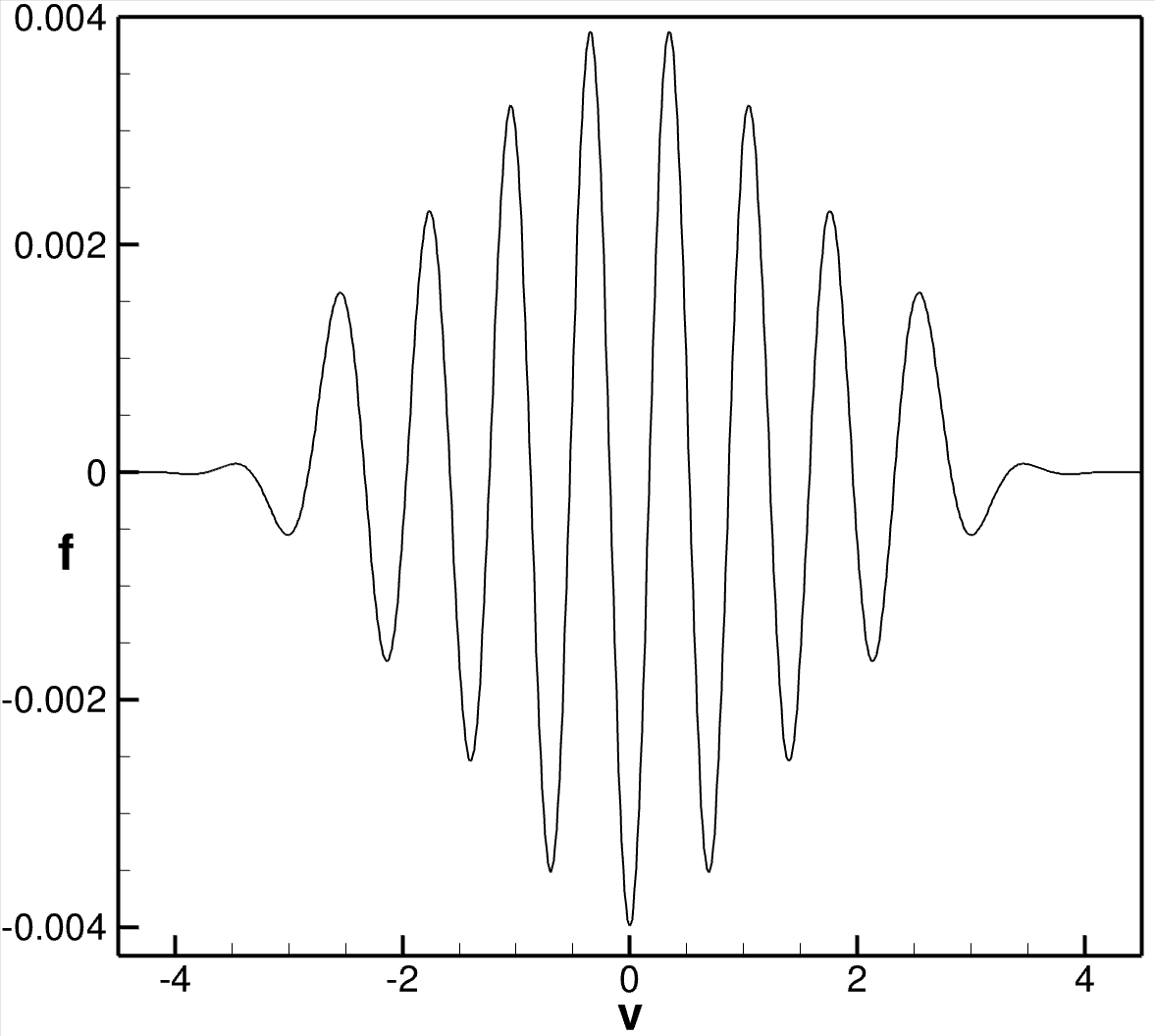
To test the accuracy and convergence of the UG method, $\mathrm{max}_{x}\,|\rho_{tot}(x,t)|$ is computed numerically and the results are plotted in Fig. 1. The numerical results were generated using the five uniform meshes $(N_{h_{x}},N_{h_{v}})=(500,400)$, $(1000,800)$, $(2000,1600)$, $(4000,400)$, $(8000,400)$, where $N_{h_{x}}$ and $N_{h_{v}}$ denote the number of partitions of the $x$-axis and the $v$-axis, respectively.

The first three meshes are such that $h_{x}\approx h_{v}$, whereas the fourth and fifth meshes are such that $h_{x}\approx h_{v}/8$ and $h_{x}\approx h_{v}/16$, respectively. The motivation for using the last two meshes comes from the fact that the problem being approximated involves only advection in the $x$-direction. Hence, it is reasonable to assume that mesh refinements in $x$ will improve the numerical accuracy as much as performing refinements in both $x$ and $v$, provided the refinement level in $v$ is sufficiently small so that the error is almost entirely due to the refinement level in $x$. Figure 1 clearly shows that the UG method is both accurate and numerically convergent under mesh refinements.

Our results compare with those of [11, 33, 54, 56] for early times where solutions are accurate, but unlike the others we do not obtain the later time recurrence that arises from periodicity of $f_{{}_{0}}(x-vt,v)$ in its first argument and the velocity mesh size used in evaluating the integral of (55). This is because of the fineness of our mesh and because of the specific dissipative properties of the DG method give monotonic error. With a mesh of $N_{h_{v}}=400$ the recurrence time is $T_{R}=2\pi k/\Delta v=\pi N_{h_{v}}/(2V_{c})\approx 126$.

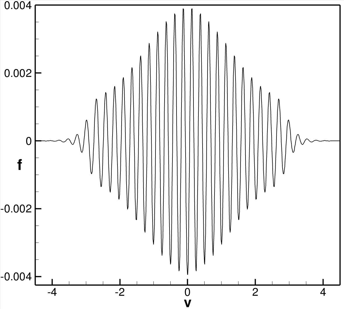
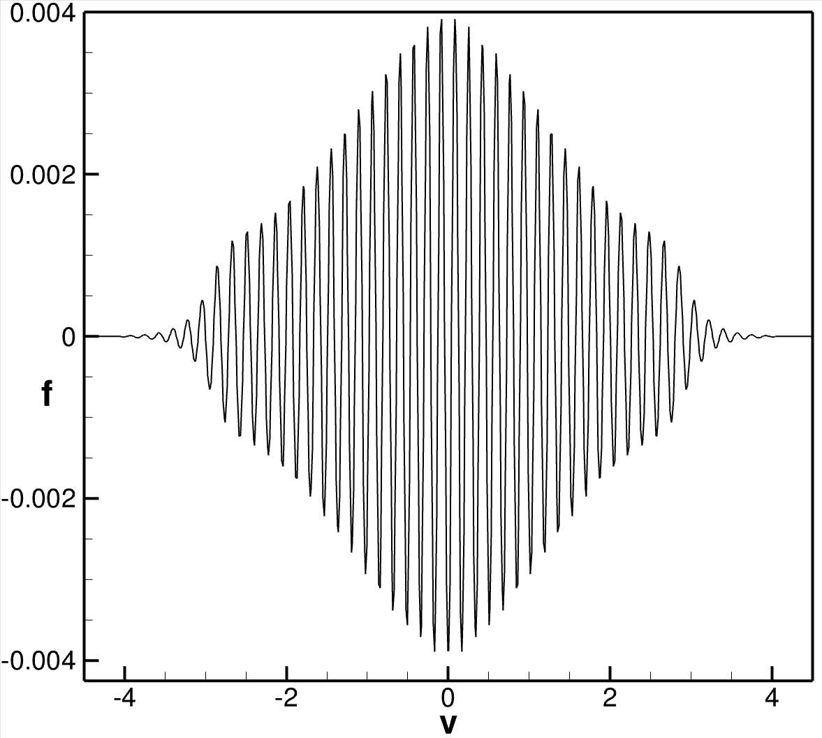
Linear advection with a Lorentz equilibrium

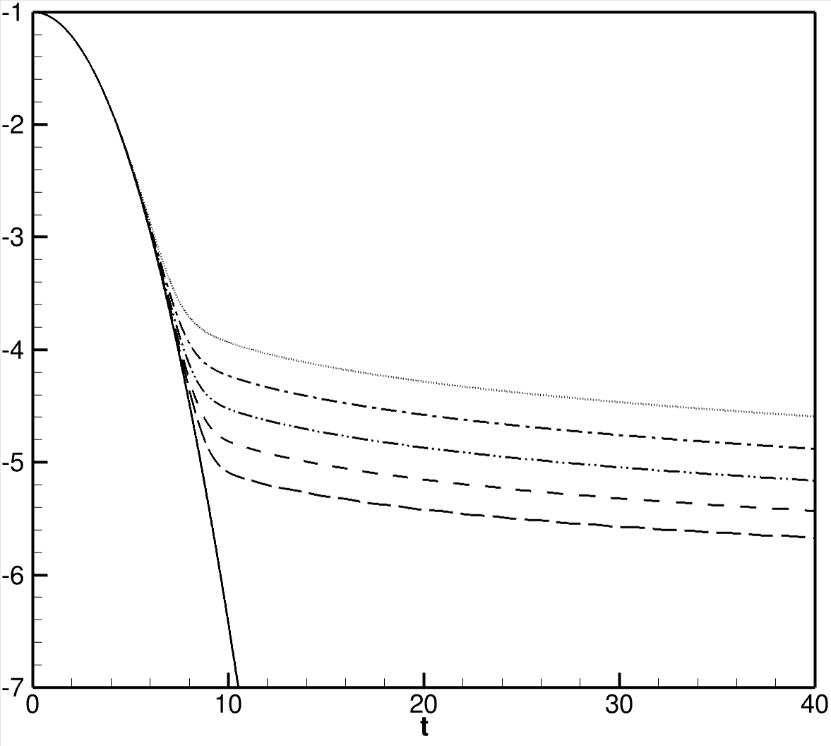
In this second example, we consider the advection problem with the Lorentz equilibrium (15). Numerical results are given for four different values of the wavenumber $k$. We will revisit these cases in Section 4.1.2, where we consider the actual Landau damping problem with the electric field not taken to be zero. Specifically, here Eq. (54) is solved for $f_{eq}=f_{L}=\pi^{-1}/(v^{2}+1)$, $A=0.01$, and the large value $V_{c}=30$ for each of the wavenumbers $k=1/8$, 1/6, 1/4, and 1/2. The corresponding values for $L$ and $T$ for $k=$1/8, 1/6, 1/4, and 1/2 are $L=16\pi$, $12\pi$, $8\pi$ and $4\pi$ and $T=75,$ 75, 50, and 50, respectively. The uniform mesh $(N_{{}_{x}},N_{{}_{v}})=(1000,2000)$ was employed in each of the four cases. For this case, it is easily shown using residue calculus that the charge density of (55) is given by

$$\rho_{tot}(x,t)\ =\ -A\cos{(kx)}\,e^{-kt}\,.$$ (60)

This implies that $\mathrm{max}_{x}\,|\rho_{tot}(x,t)|=0.01\,e^{-kt}$.

The computed results for each of the four wavenumbers $k$ are shown in Fig. 2 along with the exact result of (60). From the figure it is seen that for early times the computations match the theoretical result (60). At late times the computations diverge and, as anticipated, it is more difficult to resolve cases with larger $k$, i.e. with finer spatial structure.

Figure 1: (Linear advection with Maxwell equilibrium) Plot of $\rm{log}_{10}(\mathrm{max}_{x}\,|\rho_{tot}(x,t)|)=$ $-(\rm{log}_{10}e)t^{2}/8+1$ vs. $t$: analytic solution (solid), $(N_{h_{x}},N_{h_{v}})=$ (500,400)(dot), (1000,800)(dash-dot), (2000,1600)(dash-dot-dot), (4000, 400) (short dash), (8000, 400) (long dash).

Figure 2: (Linear advection with Lorentz equilibrium) Plot of $\rm{log}_{10}(\mathrm{max}_{x}\,|\rho_{tot}(x,t)|)=$ $-(\rm{log}_{10}e)kt+2$ vs. $t$: $k$=1/8 (top left), $k$=1/6 (top right), $k$=1/4 (bottom left) and $k$=1/2 (bottom right); analytic solution (dash), numerical solutions (solid).

4.1.2 Linear Landau Damping Results

The next two examples test the ability of the method to reproduce results consistent with the theoretical results of linear Landau damping. We emphasize that it is not enough to merely show exponential decay, but to believe an algorithm one must compare the decay rates and the parametric dependence of the theoretical rates. As above, both Maxwellian and Lorentzian equilibria are considered. For the Maxwellian equilibrium, which were previously treated in [11, 33, 36, 54, 73, 76], results are computed using four successively refined uniform meshes in order to demonstrate that the numerical decay rates converge to the theoretical decay rate under mesh refinement. For the Lorentz equilibrium, we will see that the UG method is robust in the sense that it produces the correct decay rates for different wavenumbers $k$.

As noted in Section 2, Landau showed the electric field decays exponentially in the time-asymptotic limit (for more rigor see [46] for the linear case and the recent nonlinear results of [53], of which Ref. 37 is an early version of the present work). More specifically, if we write the frequency as $\omega(k)=\omega_{R}(k)+i\gamma(k)$, where $\omega_{R}(k)$ and $\gamma(k)$ are real-valued, then in the time-asymptotic limit $E_{k}(\omega,t)$ decays at a rate $\gamma(k)$ and oscillates at a frequency $\omega_{R}(k)$.

Besides the Maxwellian equilibrium of (14), the Lorentzian equilibrium $f_{L}$ of (15) gives rise to exponential damping of the electric field. In this case, the decay rate $\gamma(k)$ for the $n$-th electric field mode with $k=2\pi n/L$ is given by

$$\gamma(k)=-k\,,$$ (61)

where $\gamma<0$ implies damping, and the corresponding frequency of the electric field oscillations satisfies

$$\omega_{R}(k)=1\,.$$ (62)

The derivation of (61)-(62) is described in Appendix A. It is important to note that formulae (61) and (62) are explicit, which directly results from using the Lorentz equilibrium, whereas, as noted above, the formula for $\gamma(k)$ and $\omega_{R}(k)$ when a Maxwell equilibrium is used are implicitly defined [42].

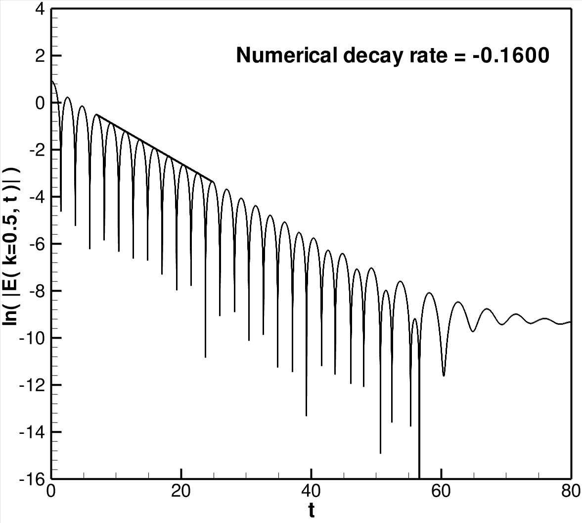
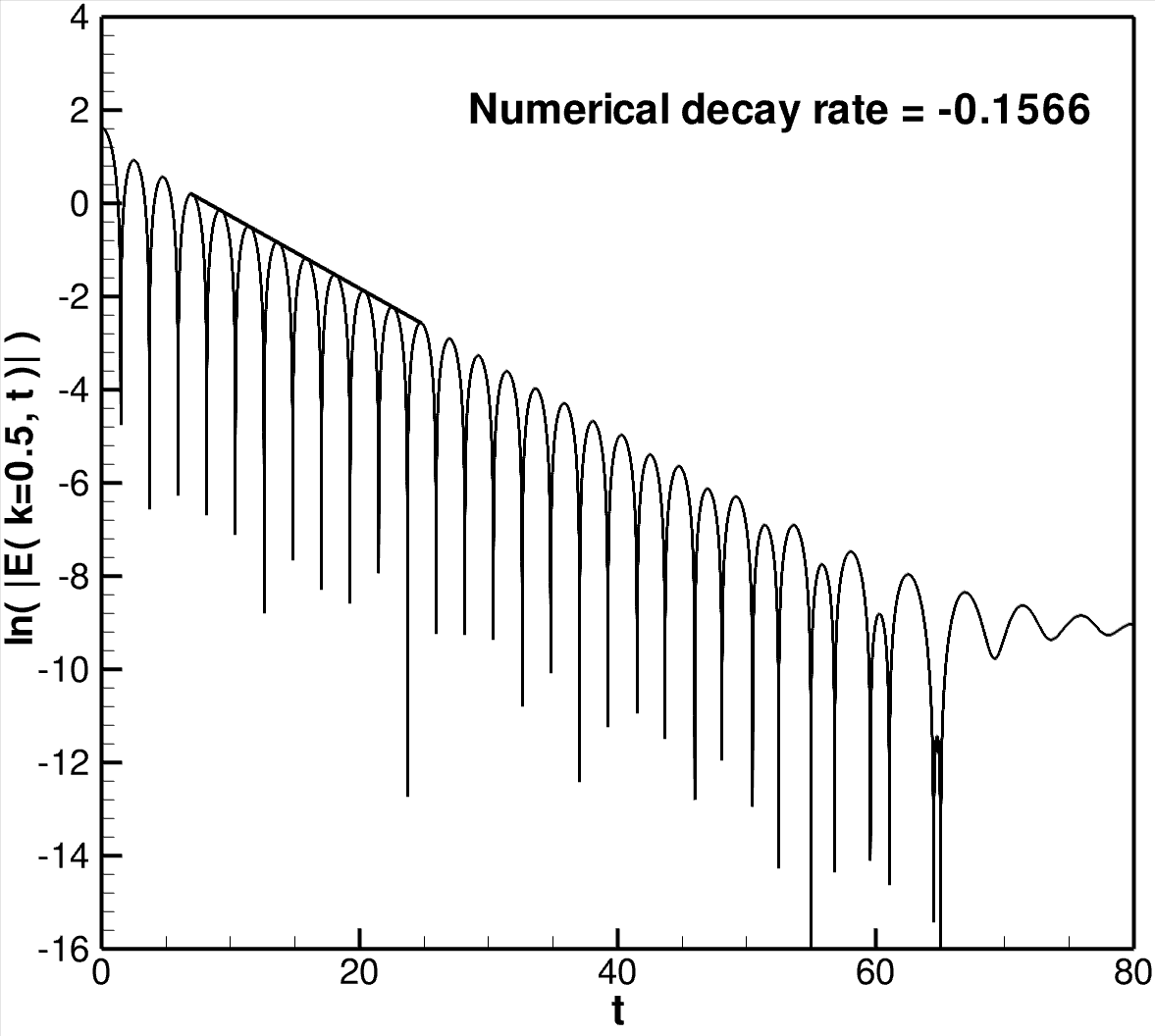
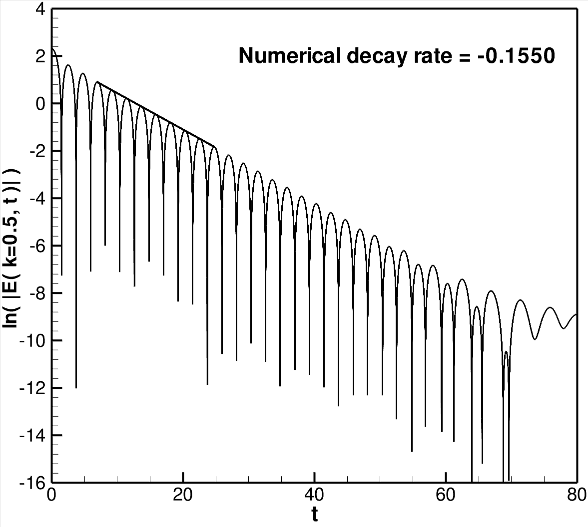
Linear Landau damping with a Maxwell equilibrium

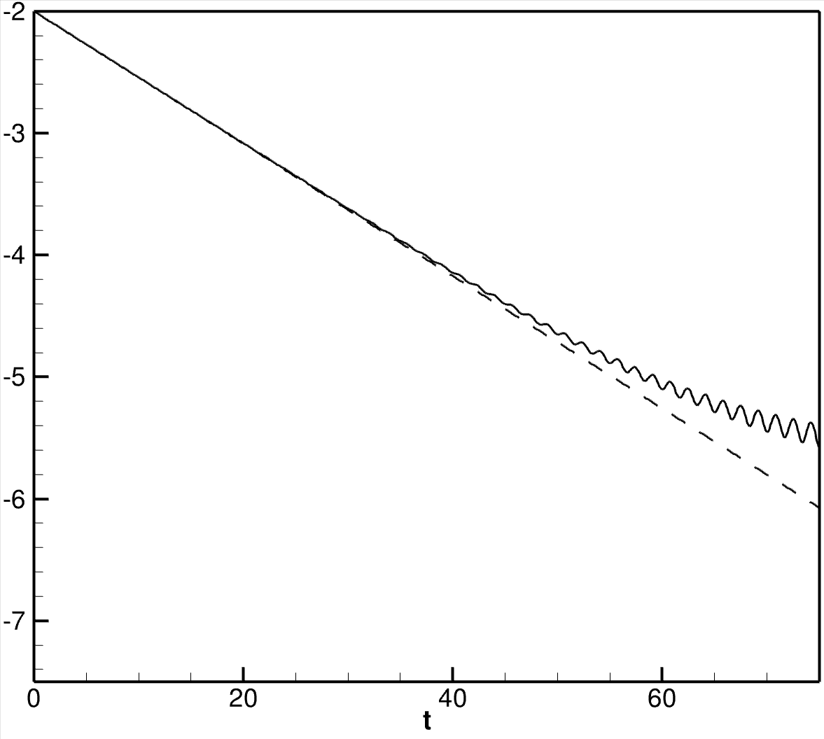
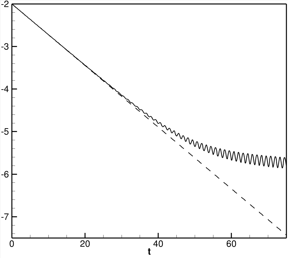
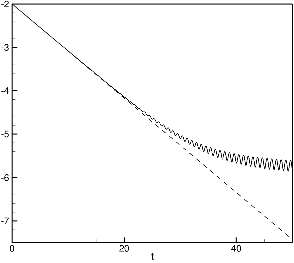
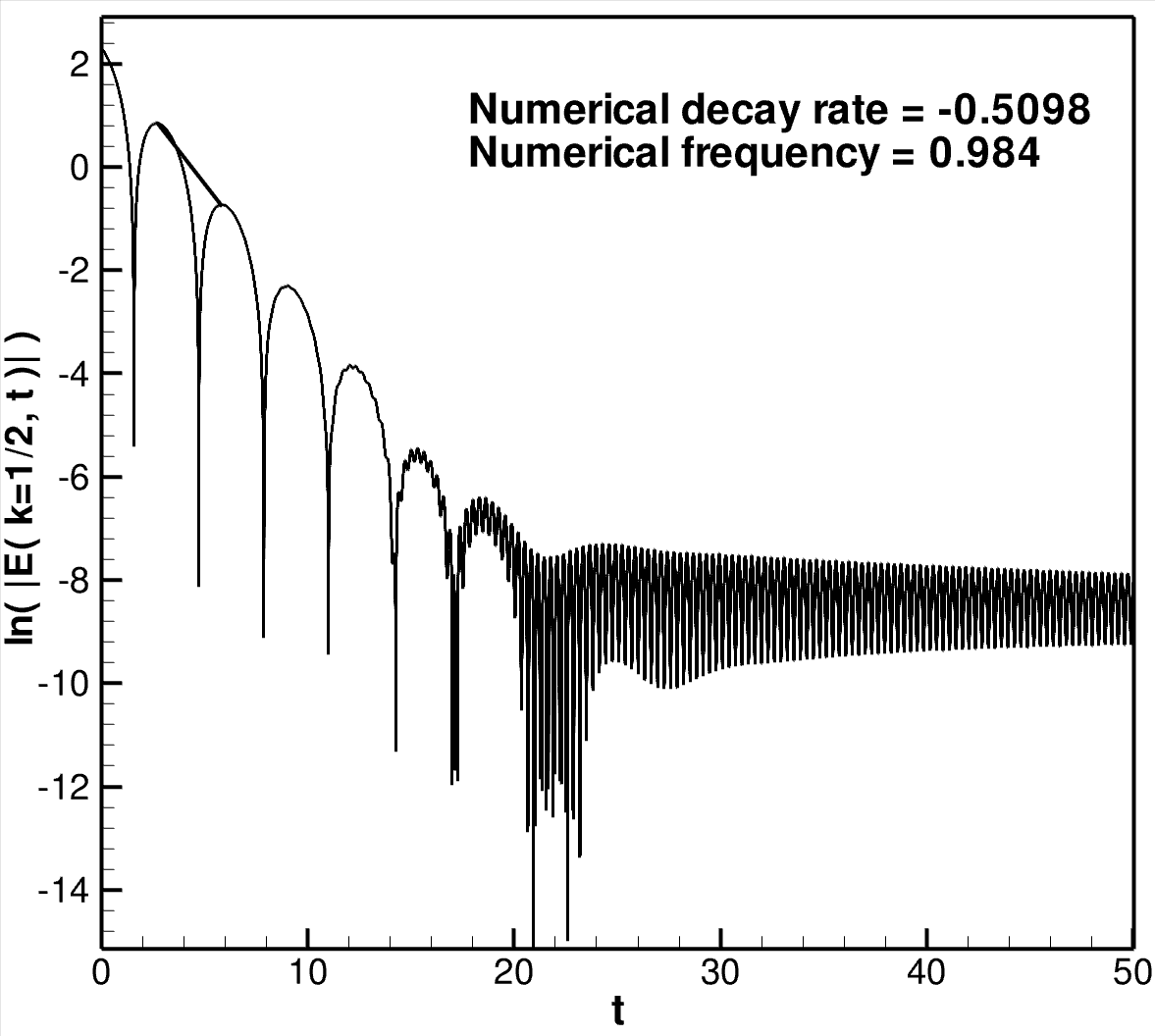
We solved the linear system (13a)-(13c) with $f_{eq}=f_{M}=(2\pi)^{-1/2}e^{-v^{2}/2}$, $A=0.01$, $k=0.5$, $L=4\pi$, $V_{c}=4.5$ and $T=80$. For this problem, the theoretical decay rate and frequency of oscillations to the third decimal digit are respectively equal to $\gamma=-0.153$ and $\omega_{R}=1.415$ [11]. Approximate solutions are computed using the four uniform meshes $(N_{h_{x}},N_{h_{v}})=(250,400)$, $(500,800)$, $(1000,1600)$ and $(2000,1600)$.

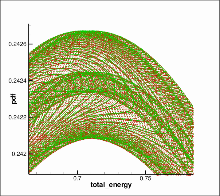
Phase-space contour plots and cross-sectional plots in $v$ of the approximate solution $f_{h}$ for $(N_{h_{x}},N_{h_{v}})=(500,800)$ and $t=0,$ $t=25$, $t=50$, and $t=75$ are displayed in Fig. 3. These sequential plots show the increase in filamentation of $f_{h}$ as time elapses.

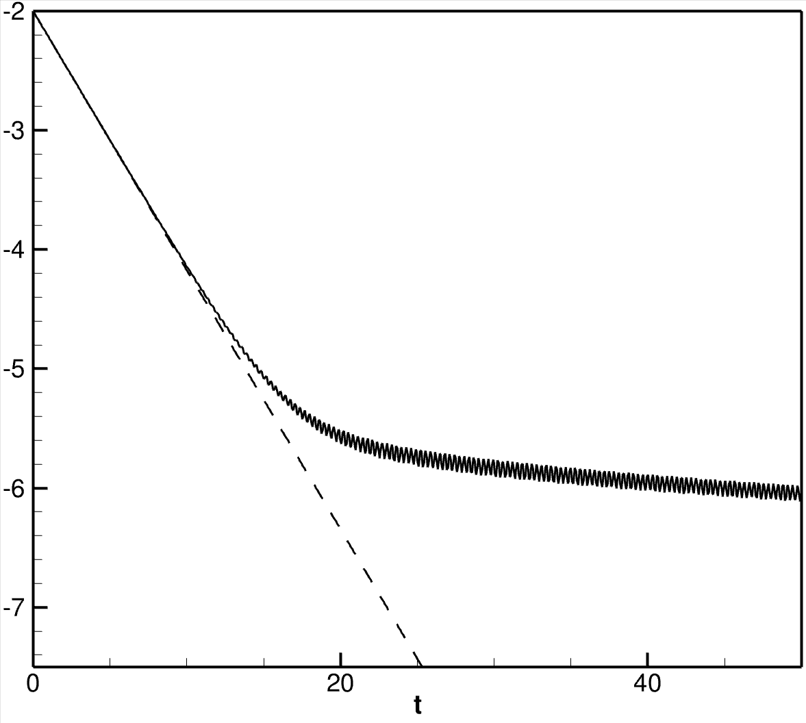
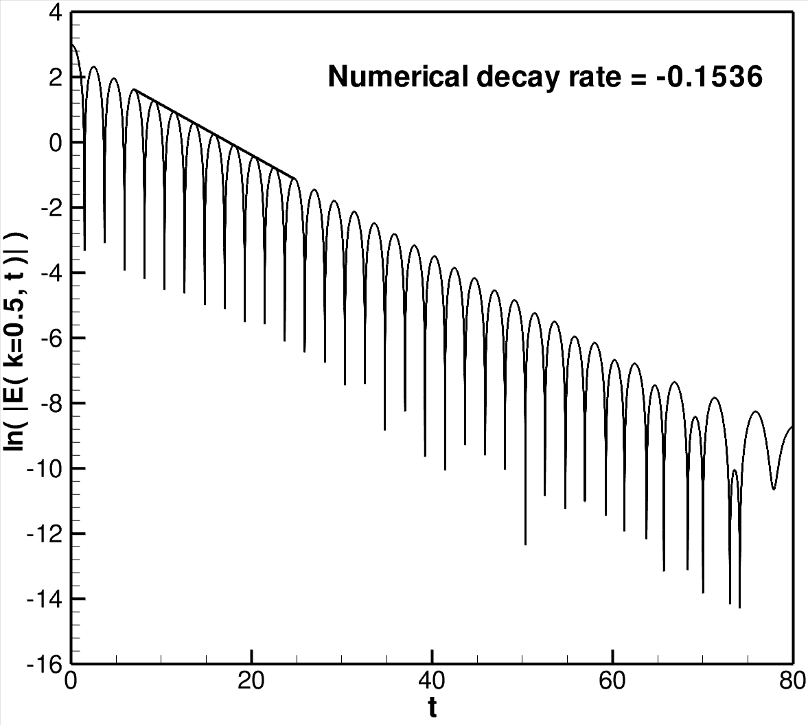
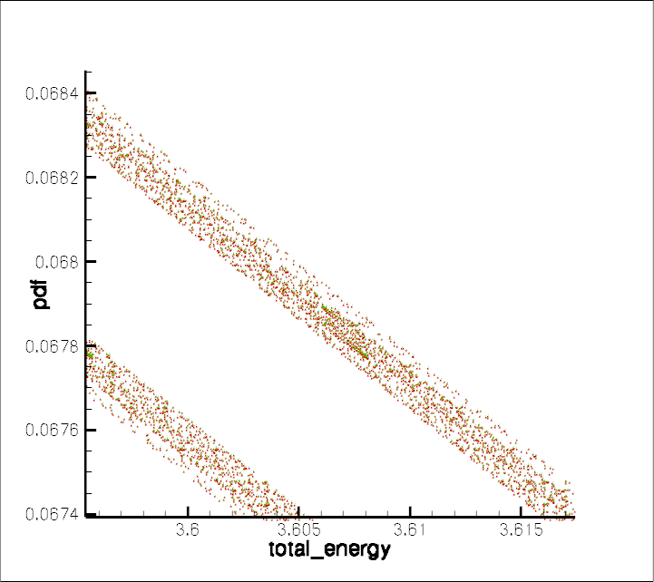
The convergence of numerical decay rates of the dominant electric field Fourier mode is demonstrated in Fig. 4. The decay rate resulting for each mesh was computed by calculating the slope of the straight line plotted in the figure. In each case, the line was defined by the point occurring at the peak of the third oscillation and the point occurring at the peak of the ninth oscillation. A time step of $\Delta t=0.001$ was used in order to ensure that the points defining each of the lines were actual computed data points rather than points that were determined using some interpolation of the data. Under mesh refinement, the numerical decay rate is seen to converge, up to three decimal-digit accuracy, to the theoretical decay rate of -0.153. In all four cases, the numerical frequency is observed to correspond to the theoretical frequency up to three decimal-digit accuracy. We also note that, upon refining the mesh, the decay of the dominant mode is sustained for longer times before leveling off. Our results compare favorably with those of previous works [11, 33, 36, 54, 73, 76], which were obtained by various other methods. Because of the fineness of our mesh we were able to proceed to longer times than all but [76] which achieved machine zero for small perturbations.

As with the advection results above, in contrast to all other works, we do not see recurrence. It is important to note that recurrence is in fact an indication of numerical error. Recurrence is a general phenomenon in finite-dimensional dynamical systems with time advancement maps that are measure preserving, one-one, onto, bicontinuous, and have a bounded phase space. Poincaré proved recurrence for finite-dimensional Hamiltonian systems, although it can hold for other systems as well. The Vlasov-Poisson system is an infinite-dimensional Hamiltonian system [49], and there is no general recurrence theorem for such systems.

Numerical truncation procedures generally are not Hamiltonian, and indeed we have shown this to be the case for the DG method used here. However, it has been shown that the DG method, although not Hamiltonian, does give a finte-dimensional system that preserves phase space volume [18] and has a bounded energy. Thus our semi-discrete system has all the ingredients for making a general estimate for the recurrence time for the distribution function in terms of the number of degrees of freedom, like that done by Boltzmann for gas dynamics. This results is a very long time for meshes with any significant resolution. Note, this approach differs from a result that is often quoted in numerical works that follows for the method of [11]; viz.  for a given Fourier mode and a mesh of size $\Delta v$ the advection equation was shown to have a recurrence time for the electric field of $T_{R}=2\pi k/\Delta v$. Many Vlasov algorithms see recurrence at a value that is close to this advection value $T_{R}$. It is important to note that this does not mean that the distribution function is recurring in phase space on this time scale. In [18] we present detailed recurrence calculations for our DG algorithm with piecewise constant and higher order polynomials.

In any event, recurrence is not physical and the same can be said for the non-recurrent flattening of the electric field decay rate that is seen in our results with the DG algorithm at late times. The lack of recurrence in our results is due to both the very fine mesh size as well as the dissipative nature of DG algorithms, which is monotonic in nature. However, from Fig. 4 (and also Fig. 5 below) we would argue that DG can do a good job.

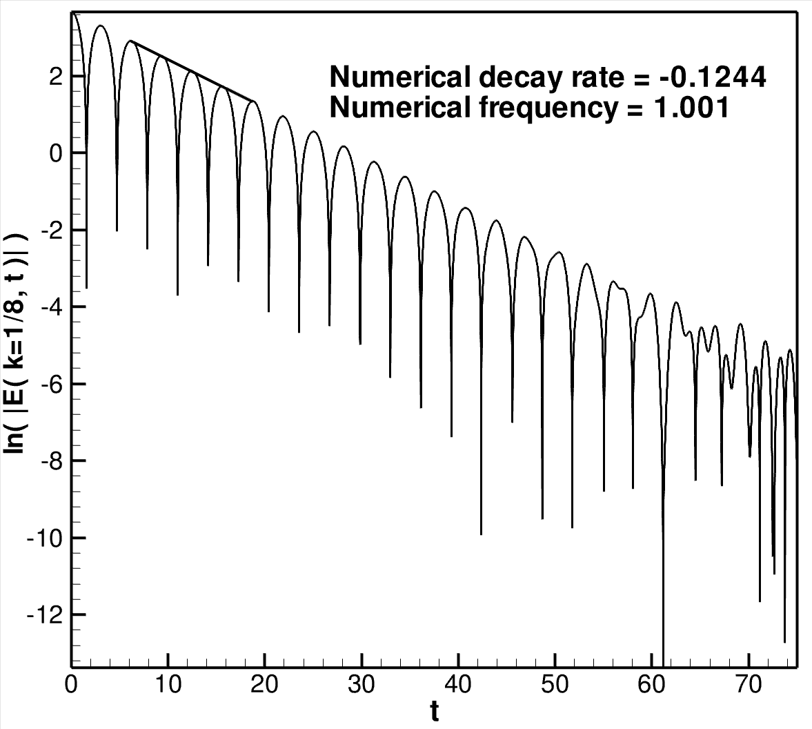
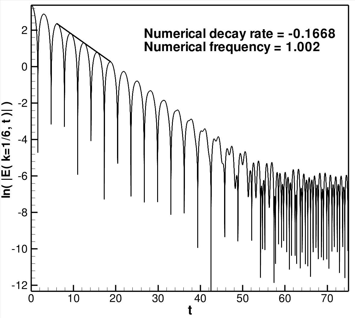
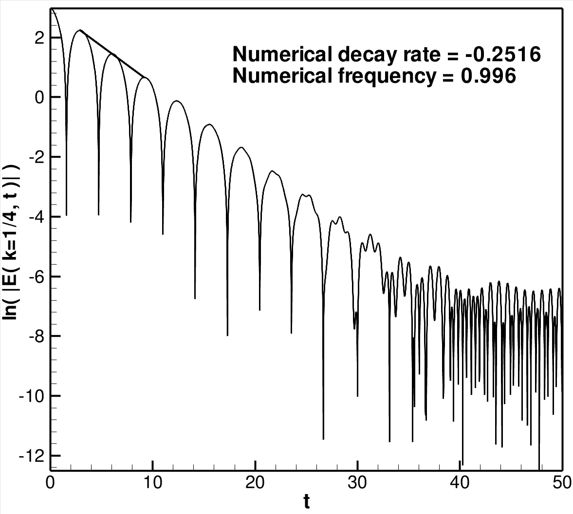
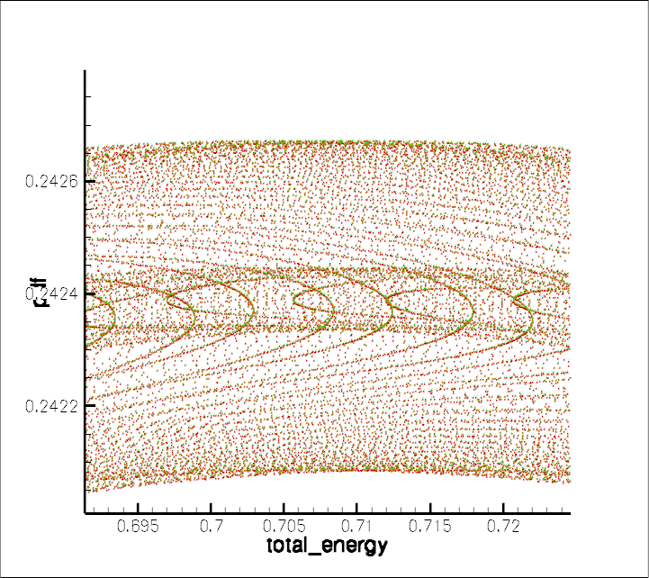
Linear Landau damping with a Lorentz equilibrium

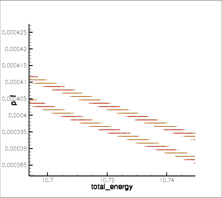
The ability of the UPG method to achieve accurate damping results across different wavenumbers is now investigated. As noted above, the Lorentz equilibrium is used in this example because explicit formula for the electric field damping rates and the frequencies of the damped oscillations are easily obtained (see Appendix A). Moreover, this example also tests the ability of the method to produce accurate results for an equilibrium that has a much heavier tail in $v$ than does the Maxwell equilibrium. The heavy (algebraic) tail of the Lorentz equilibrium leads to a faster rate of filamentation because there are more resonant electrons than for the Maxwell equilibrium.

The linear system (13a)-(13c) is solved with ${f}_{eq}=f_{L}=\pi^{-1}/(v^{2}+1)$, $A=0.01$, and $V_{c}=30.$ for each of the wavenumbers $k=1/8$, 1/6, 1/4, and 1/2. Note, $V_{c}$ needs to be large because of the algebraic tail of $f_{L}$. The corresponding values for $L$ and $T$ for $k=$1/8, 1/6, 1/4, and 1/2, are $L=16\pi$, $12\pi$, $8\pi$ and $4\pi$ and $T=75,$ 75, 50, and 50, respectively. Uniform meshes were employed in all four cases, where in each case $(N_{{}_{x}},N_{{}_{v}})=(1000,2000)$.

In Fig. 5, log plots of $\rho_{tot}$ for the four cases are given. The observed damping for $k=1/2$ lasts for a shorter time duration than does the damping for the other three wavenumbers, even though the mesh for $k=1/2$ has the finest resolution in $x$. This result is due to the fact that the filamentation in the velocity direction develops more rapidly than it does in the other three cases. From (61), obtained in Appendix A, it follows that for a given wavenumber $k$ the fundamental mode of the electric field damps exponentially in time at a rate equal to $\gamma(k)=-k$ and the frequency for all of the damped oscillations is $\omega(k)=1$. Therefore, the theoretical damping rates corresponding to $k=1/8$, 1/6, 1/4, and 1/2 are $\gamma(k)=-1/8$, -1/6, -1/4, and -1/2. In all of the four cases shown in Fig. 5, the numerical damping rates and frequencies of oscillation are equal to the theoretical values up to the first two decimal digits.

Figure 3: (Linear Landau damping with Maxwell equilibrium) Contour plots (left) and cross-sectional plots (right), $x=2\pi$, for $\delta f$ at $t=0$, $t=25$, $t=50$, $t=75$ (descending order).

Figure 4: (Linear Landau damping with Maxwell equilibrium) Time decay plots of fundamental mode (with arbitrary ordinate origin) under mesh refinement: $(N_{h_{x}},N_{h_{v}})=$(250, 200) (top left), (500, 400) (top right), (1000, 800) (bottom left) and (2000, 1600) (bottom right). The numerical decay rate converges to the theoretical value of -0.153 to within three decimal-digit accuracy; similarly, the numerical oscillation frequency agrees with the theoretical frequency of $\omega_{R}=1.415$ to within three decimal digits.

Figure 5: (Linear Landau damping with Lorentz equilibrium) Time decay plots of fundamental modes (with arbitrary ordinate origin): $k$=1/8 (top left), $k$=1/6 (top right), $k$=1/4 (bottom left) and $k$=1/2 (bottom right).

4.2 Nonlinear Results

Two nonlinear calculations are performed, an example of strong nonlinear Landau damping and a version of the two-stream instability that we examine in greater detail. In the former case, in addition to early time damping, we expect to see motions on the bounce time scale due to particle trapping, while in the latter we expect to see trapping and an asymptotic approach to a BGK state.

4.2.1 Nonlinear Landau Damping

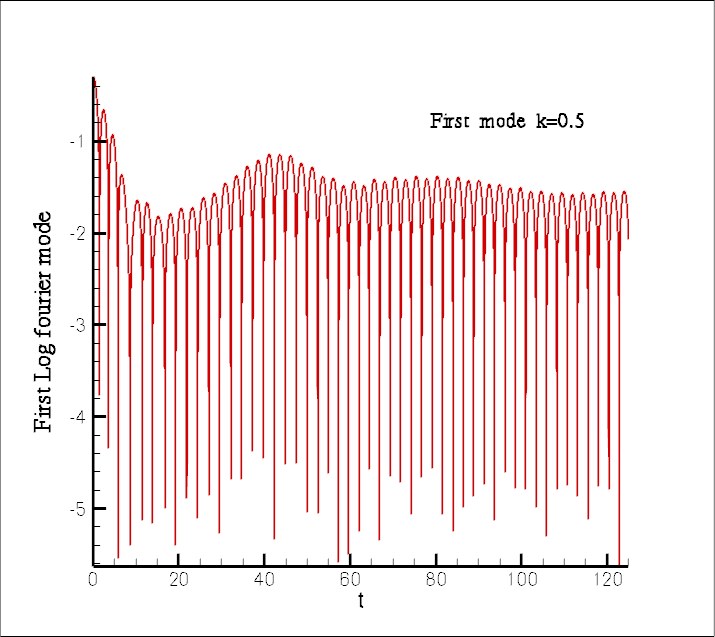
Following [11, 26, 31, 33, 41, 54, 73, 76] we consider an initial condition near a Maxwellian and of the form given by (52) and (53a)–(53c) with $f_{eq}=f_{M}=(2\pi)^{-1/2}e^{-v^{2}/2}$, $A=0.5$, $k=0.5$, $L=4\pi$, $V_{c}=5.0$ and a run time of $T=120$. Unlike the case considered in Section 4.1.2 we evolve under the full nonlinear Vlasov equation. Solutions are computed using a uniform mesh with $(N_{h_{x}},N_{h_{v}})=(1000,750)$.

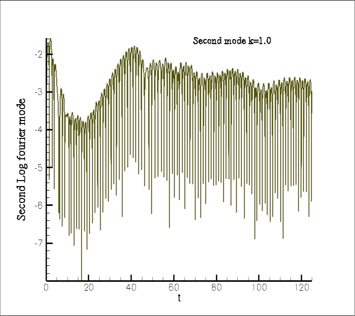
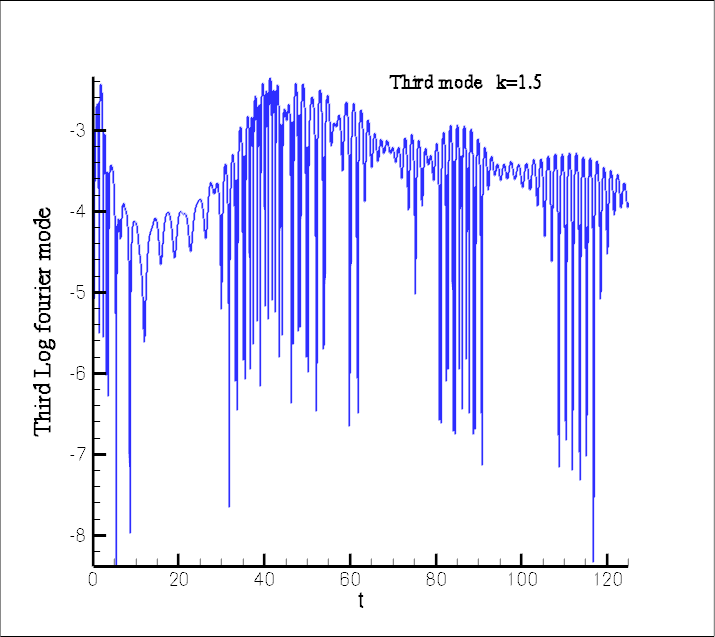
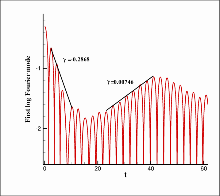
Because $A$ has been increased to $0.5$, higher modes are excited at very early times and the damping rate significantly exceeds the linear rate of $\gamma=-0.153$. This is because energy leaves the first mode as the higher modes get excited; i.e., in addition to the phase mixing process there is an energy transfer process caused by the nonlinear interaction of the modes. Figure 6 shows the amplitudes of the first four modes as a function of time, with a form similar to previous calculations. These plots are obtained from our mesh data by using the following ‘log Fourier Mode’ function:

$$\log FM_{k}(t)=\log_{10}\left(\sqrt{\left|E_{s,k}(t)\right|^{2}+\left|E_{c,k}(t)\right|^{2}}/L\,,\right)$$ (63)

with

$$E_{s,k}(t):=\int_{0}^{L}\!dx\,E(x,t)\sin\left(\frac{2\pi kx}{L}\right)$$ (64)

and

$$\ \ E_{c,k}(t):=\int_{0}^{L}\!dx\,E(x,t)\cos\left(\frac{2\pi kx}{L}\right)\,,$$ (65)

where $k$ is the mode number sought. From Fig. 6 it is seen that mode-one reaches its minimum value at around $t\approx 15$ and then all modes grow until they reach their maxima at $t\approx 40$, consistent with previous calculations. Using the maximum amplitude of mode-one, the bounce time is calculated to be $T_{B}\approx 20$ and this is also in agreement with previous results.

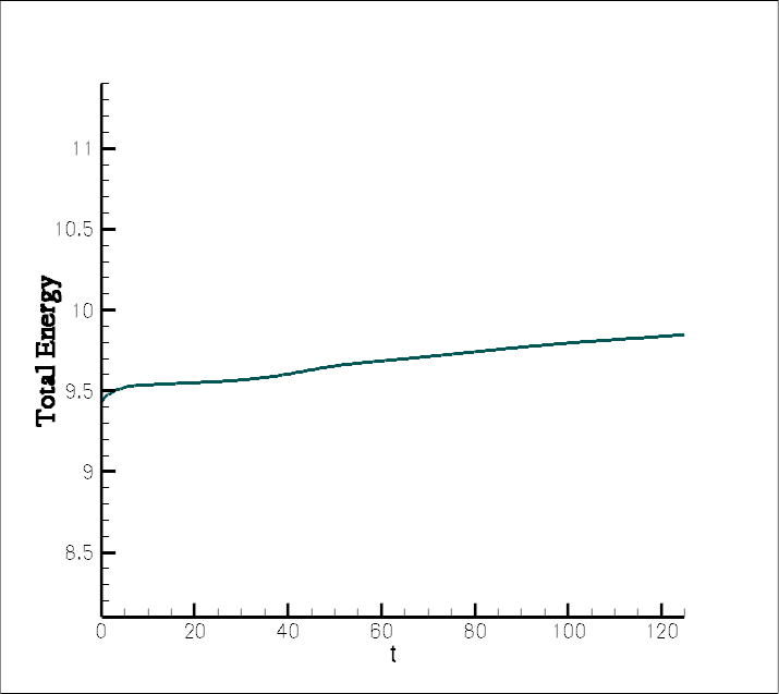
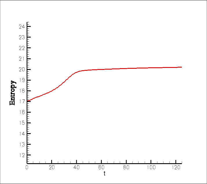
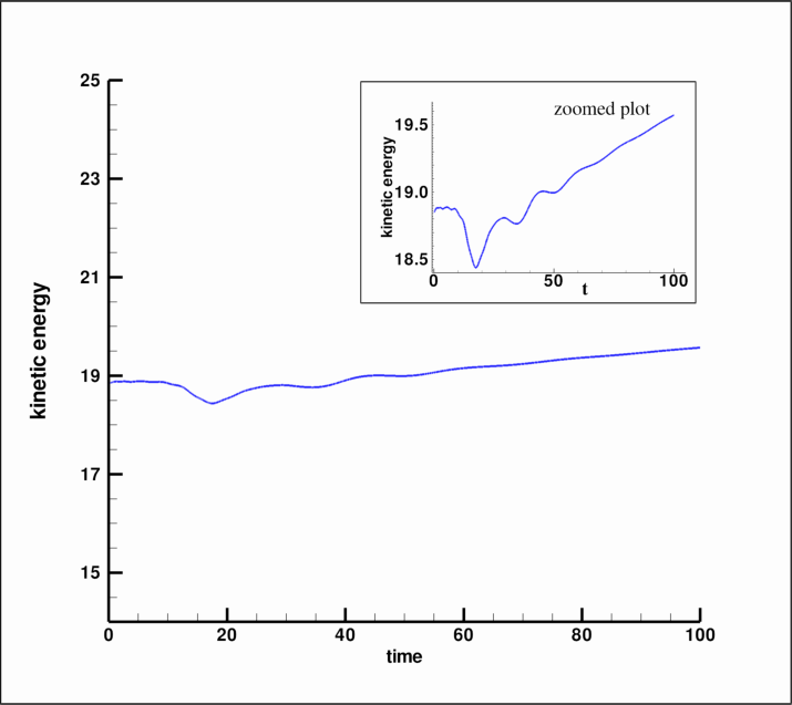
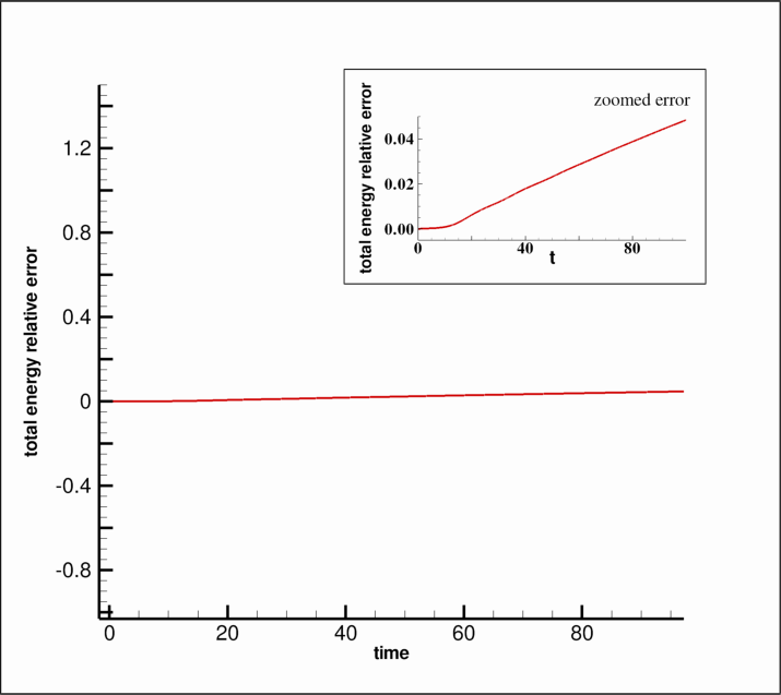
Examination of Fig. 7 reveals that we obtain a damping rate for the first mode of about $\gamma=-0.287$, a value consistent with the $-0.281$ obtained by [11] and $-0.243$ by [73], given the different ways authors have used to make this kind of fit. Also, given that we have a finer mesh, some deviation could be due to our more precise coupling to the higher modes. Examination of Fig. 8 shows there is significant entropy [(11) with $\mathcal{C}=-f\ln f$)] dissipation at short times, as also seen by [33], and this introduces some error. Also note, we have run to $T=120$, which is significantly longer than previous calculations and a small decay in all four of the amplitudes is seen. This could be due to transfer to higher modes, cascading, or due to dissipation in the algorithm. Over the full length of the run the total energy $H$ of (10) is c onserved to within a few percent, and in the later part of the run entropy is well conserved. This is improved in the next section, where we treat the two-stream instability, by decreasing the mesh size.

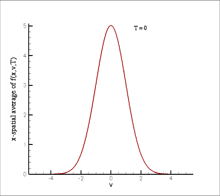
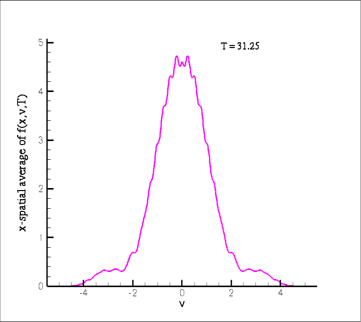
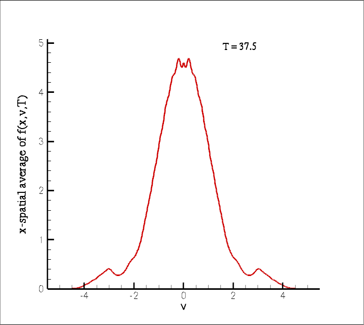
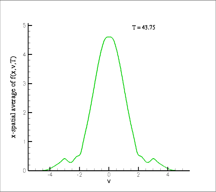
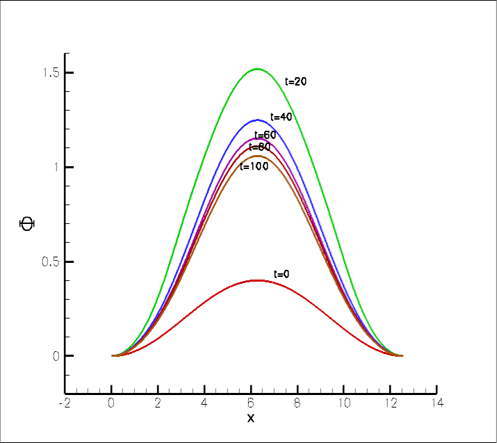
In Fig. 9 we plot the spatial average of the distribution function. Like other authors, we obtain early plateau formation in the vicinity of the phase velocity of the wave, seen in panel (b), which broadens as the higher order modes are excited. At around $t=40$, approximately the time of the first bounce maximum, significant smoothing takes place and the system settles into a nearly constant average state with a persistent electron hole. The smoothing at $t\approx 40$ can also be seen in the results of [11, 33]. Finally, we note the presence a small periodic dimpling behavior at the maximum that persists for late times.

(a) $k=0.5$.

(b) $k=1.0$.

(c) $k=1.5$.

(d) $k=2.0$.

Figure 6: (Nonlinear Landau damping with Maxwell equilibrium) Amplitudes of the first four modes versus time. Mesh size $(N_{x},N_{v})=(1000,750)$.

Figure 7: (Nonlinear Landau damping with Maxwell equilibrium) Initial damping of dominant mode followed by growth due to particle trapping.

(a) Energy.

(b) Entropy.

Figure 8: (Nonlinear Landau damping with Maxwell equilibrium) The total energy $H$ of (10), kinetic plus electrostatic, and entropy, (11) with $\mathcal{C}=-f\ln f$, versus time.

(a) $t=0$.

(b) $t=12.5$.

(c) $t=31.5$.

(d) $t=43.75$.

(e) $t=75$.

(f) $t=112.5$.

Figure 9: (Nonlinear Landau damping with Maxwell equilibrium) Spatial average of the distribution function at the times indicated.

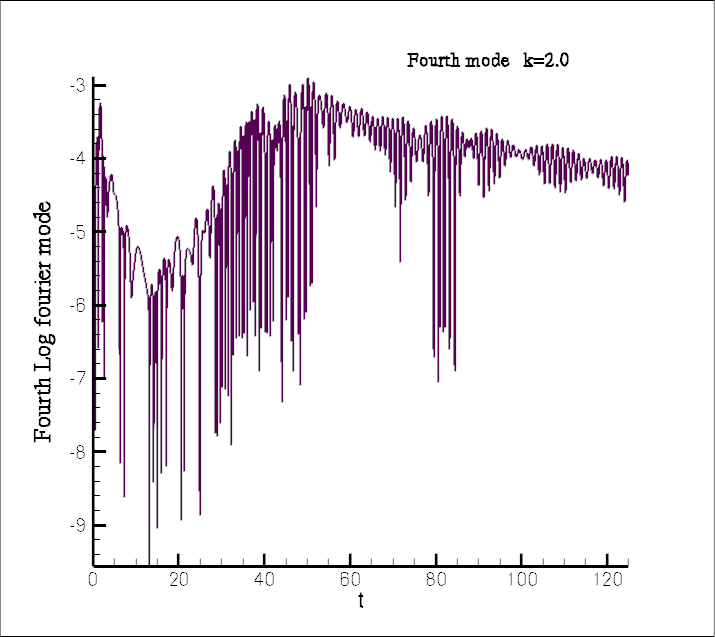
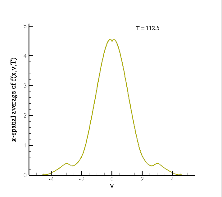
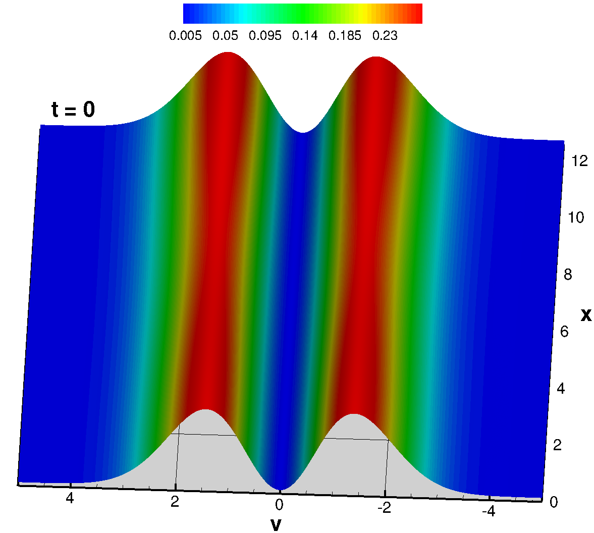
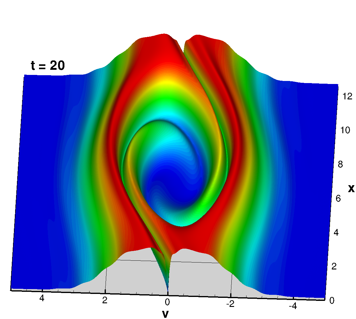
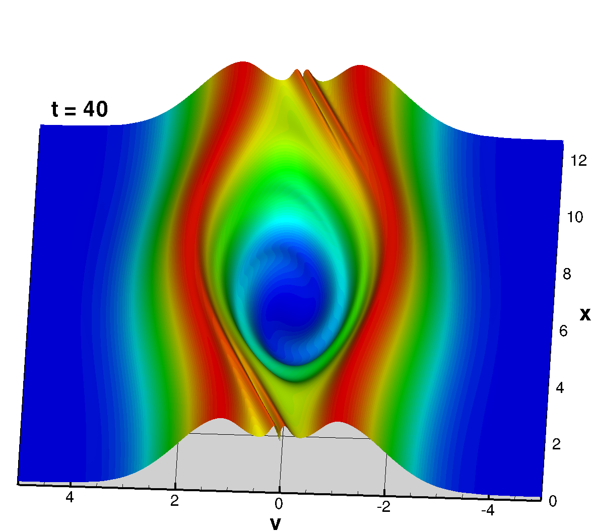
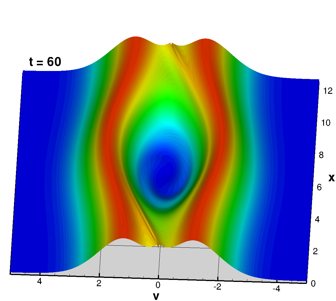
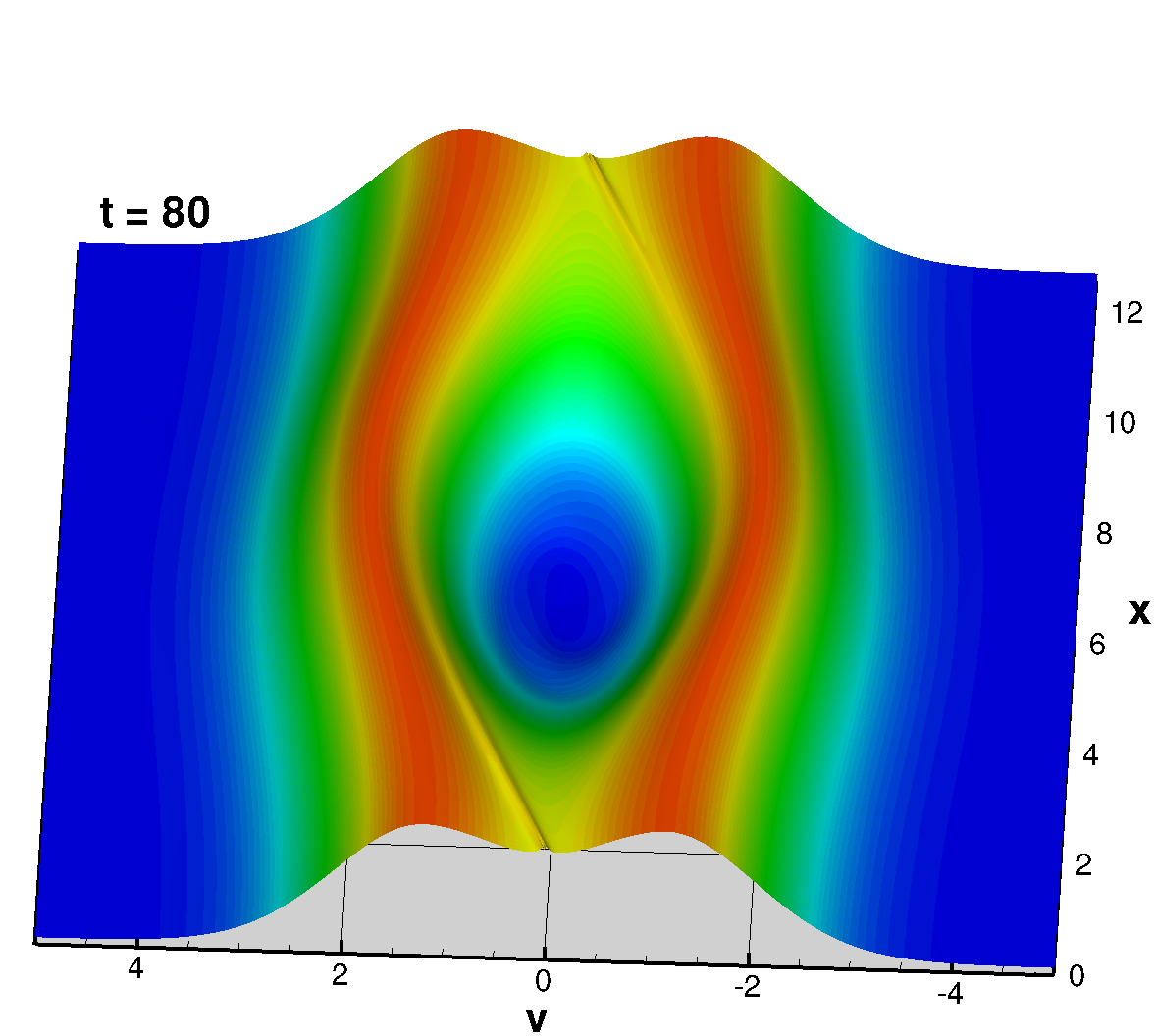
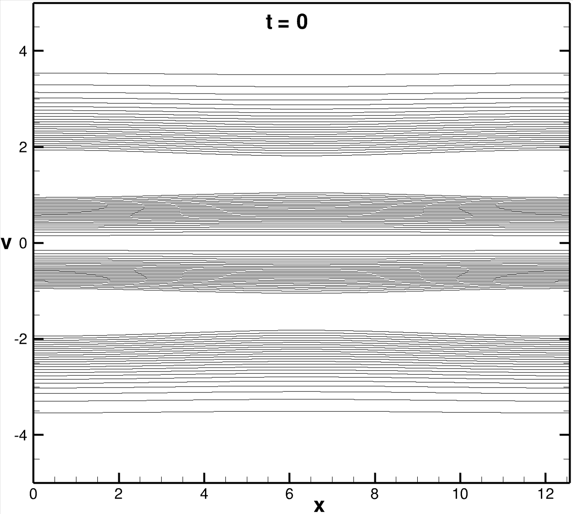
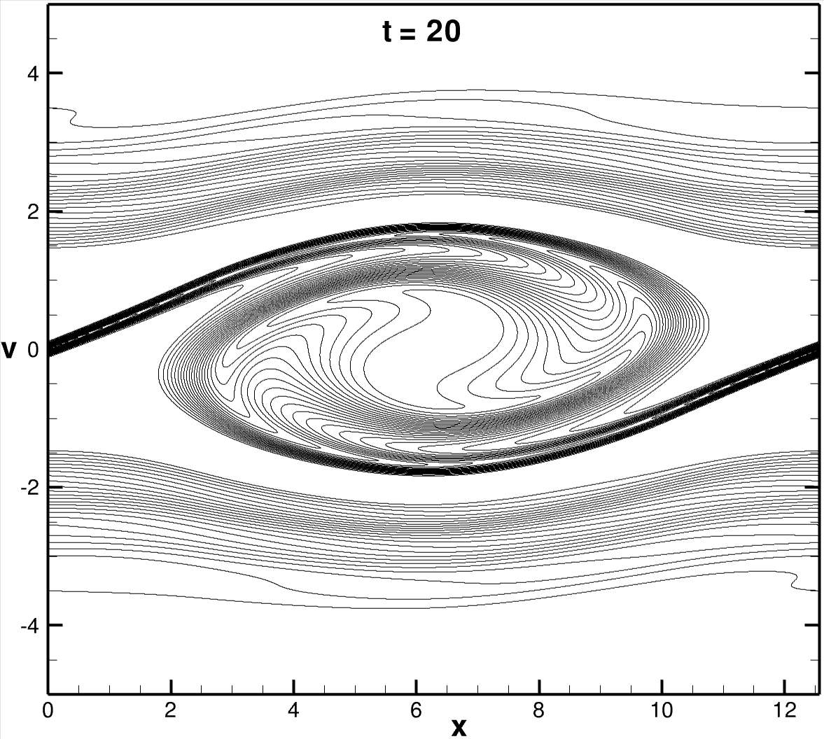
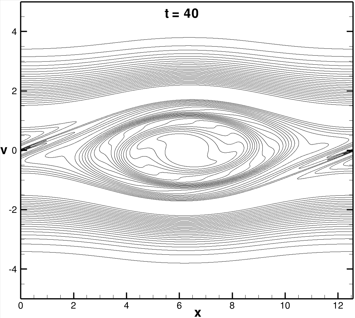
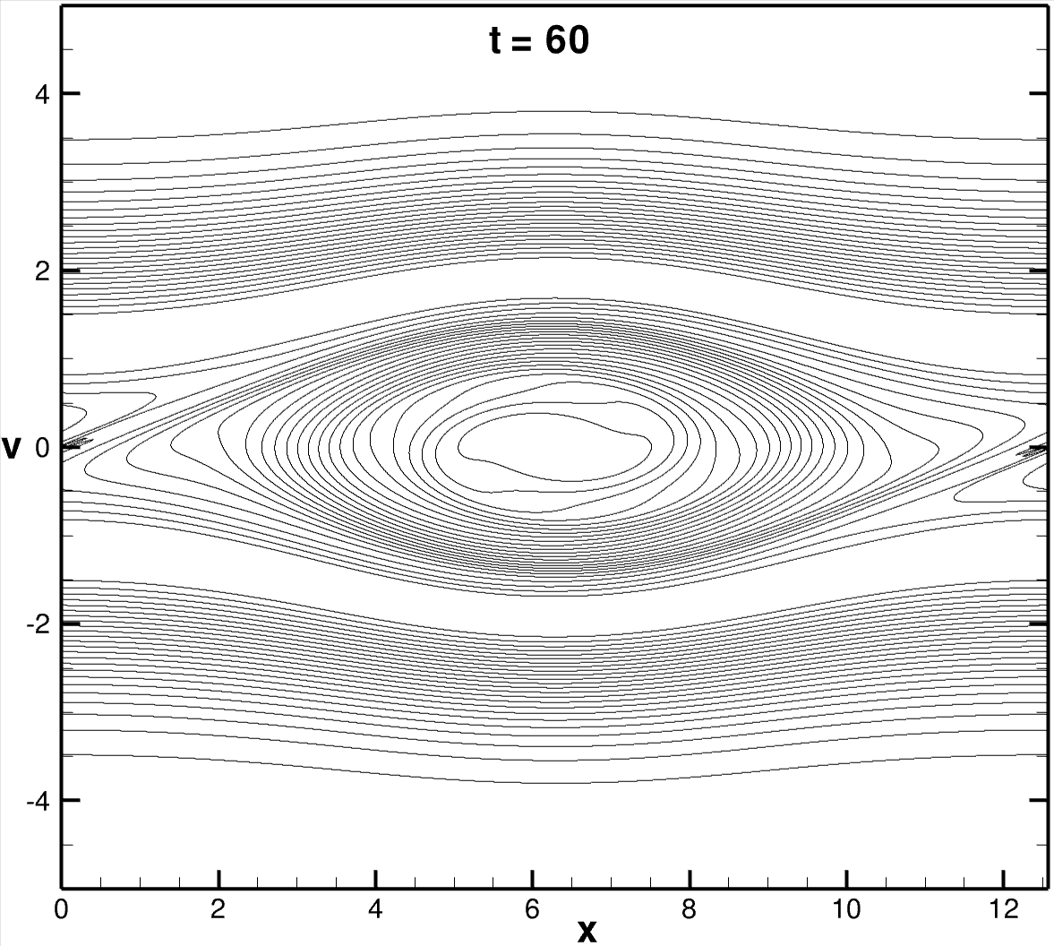
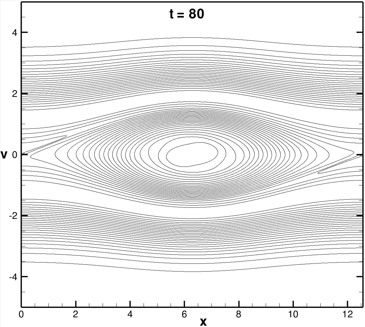
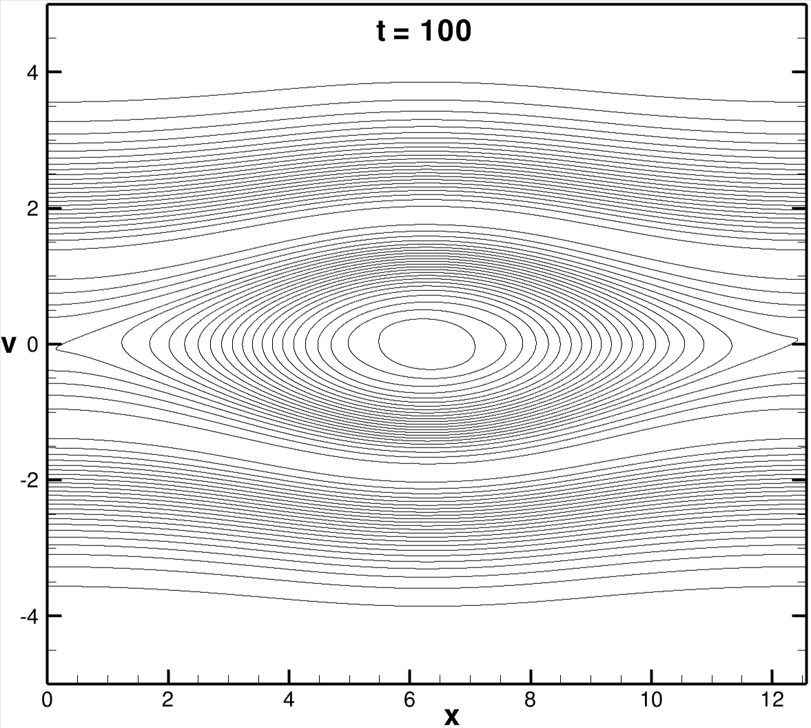
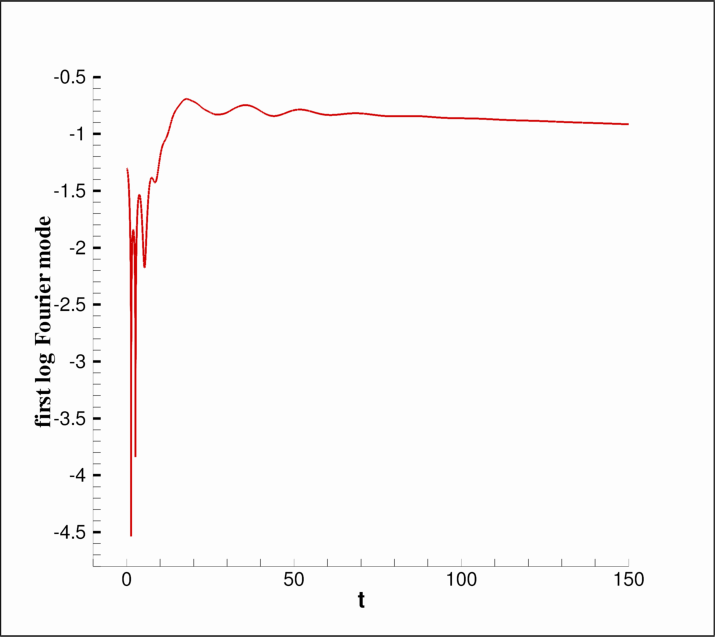
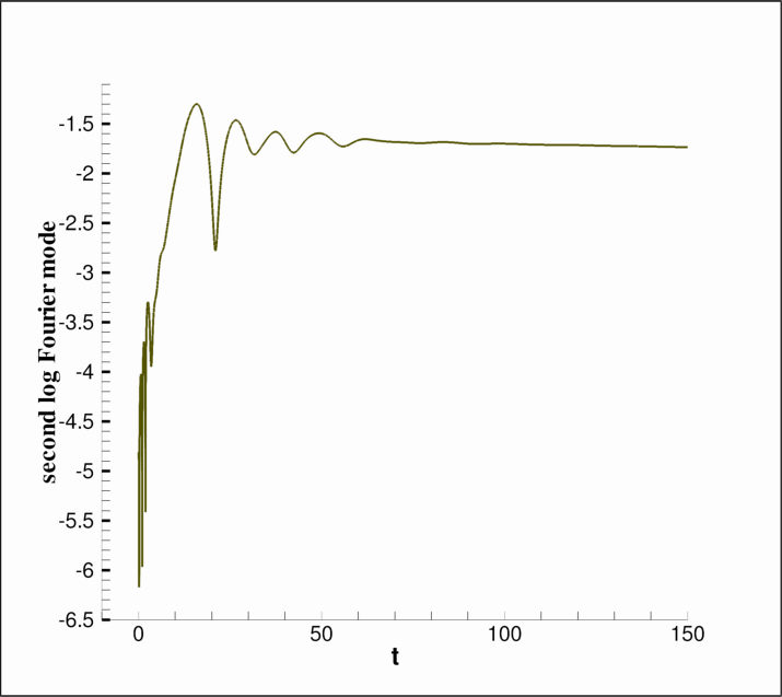
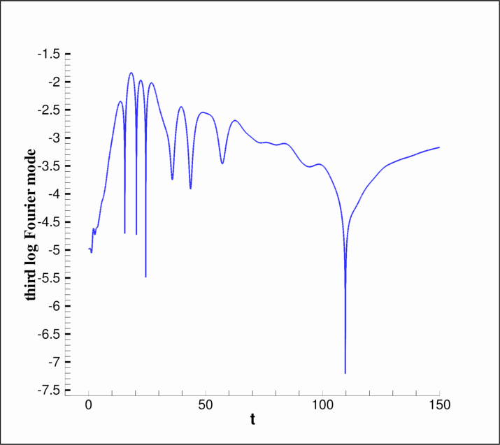
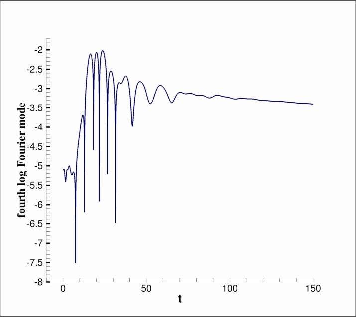
4.2.2 Nonlinear Two-Stream Instability

In this subsection, we numerically study the long-time nonlinear evolution of the two-stream instability, a standard example that has been used for demonstrating the efficacy of a variety of numerical algorithms [11, 29, 36, 41, 54, 56, 73]. Like these previous calculations, we consider the equilibrium state

$$f_{TS}(v)\ =\ \frac{1}{\sqrt{2\pi}}\,v^{2}\,e^{-v^{2}/2}\,$$ (66)

and apply our algorithm to the nonlinear system (12a)-(12c) with data of the form given by (52) and (53a)–(53c). We choose parameters values to be $A=0.05$, $k=0.5$, $L=4\pi$, $V_{c}=5$, and $T=100$, a uniform mesh defined by $(N_{x},N_{v})=(1800,1400)$, and a time step $\Delta t=0.00125$.

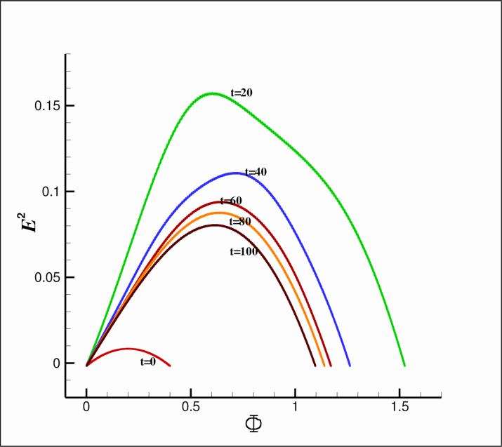
Qualitative Behavior

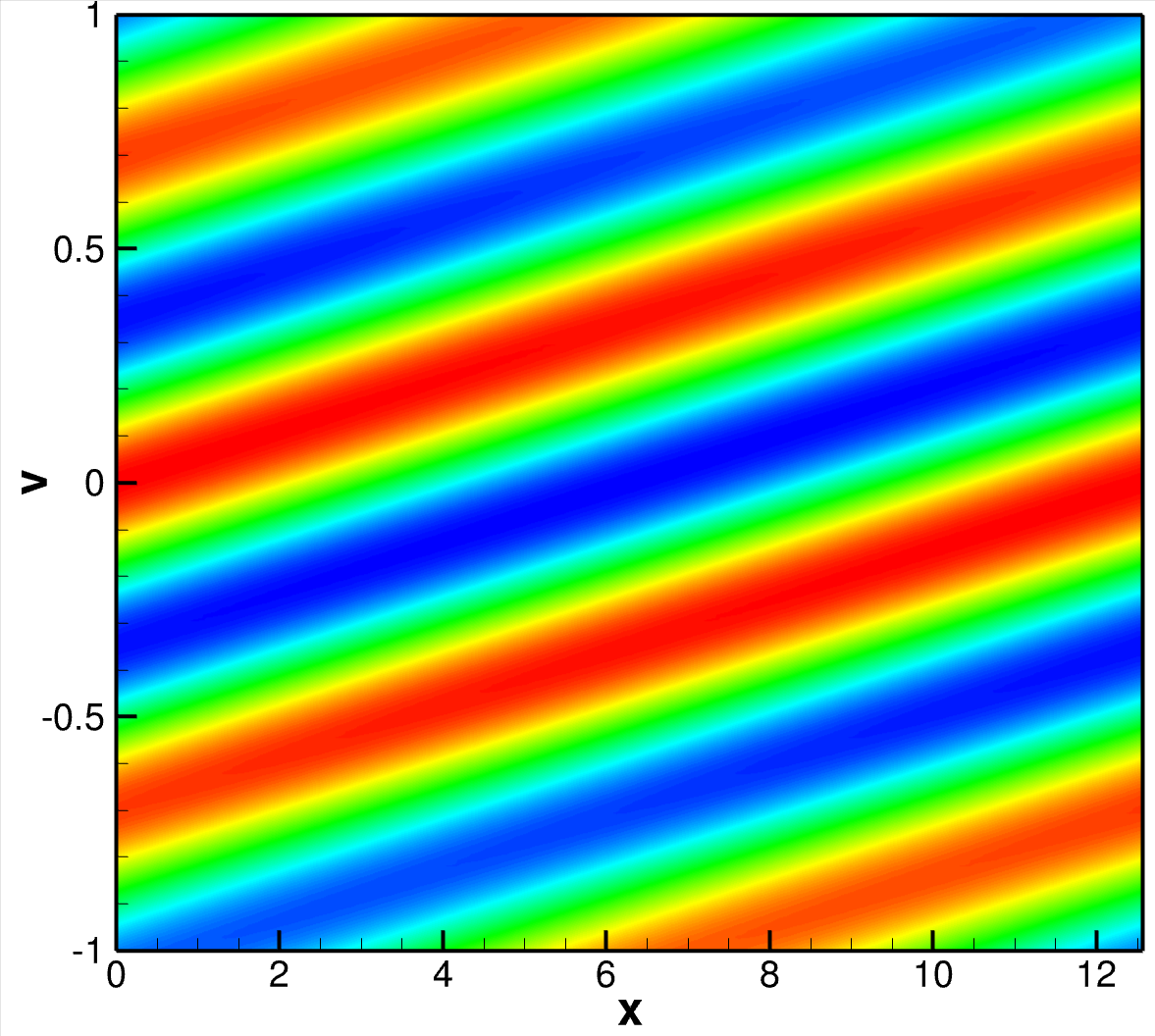
Figures 10 and 11 show 3D and 2D contour plots of the distribution function $f$ in phase space at different instances of time. The initial data consists of two symmetric, counter-streaming, warm beams with the small sinusoidal perturbation superimposed, as described above. We obtain the qualitative behavior expected: the linear two-stream instability grows exponentially until nonlinearity becomes important and trapping occurs, with an eventual long time asymptotic Bernstein-Greene-Kruskal (BGK) state [8] with an apparent electron hole-like structure (cf. e.g.  [60]). As the nonlinear system evolves, linear modes grow and saturate as shown in Fig. 12, the phase space hole forms as a portion of the electron distribution becomes trapped and exhibits filamentation. Over time, the sharp contour variation associated with filamentation is smoothed out, a consequence of nonlinearity and the numerical dissipation of the UPG method. (We note, here for aesthetic reasons some smoothing was also done by the plotting routine.) Our numerical results are indicative of a very stable computational scheme. This is partly due to the fact that our DG method is monotone and mass conservative. The particle number error accumulation in time is due to the nonlinear coupling.

Early Growth

As noted above, Fig. 12 shows the time evolution of the first four modes, which have wavenumber values $k=0.5$, $k=1$, $k=1.5$, and $k=2$, from $t=0$ to $t=T=100$. (Recall, our domain is of size $4\pi$.) At early times, $0\leq t<20$, the behavior illustrated in Fig. 12 is consistent with the results of previous authors where the initialized mode-one with $k=0.5$ dominates the other modes that are not initially excited. All modes reach a maximum at $t\approx 18$ with growth rates on the order of a couple of tenths of $\omega_{p}$ which is typical of linear theory for this problem. During early times, noise in the system and the growth of mode-one excites the other modes as was the case for the nonlinear Landau damping of Section 4.2.1. A comparison was made in the calculations of [29] using results from [36], but we give some further details here.

The plasma dispersion function from Vlasov linear theory is given by

$$\epsilon=1-\frac{1}{k^{2}}\int_{-\infty}^{\infty}f_{0}^{\prime}(v)\frac{dv}{v-\omega/k}\,,$$ (67)

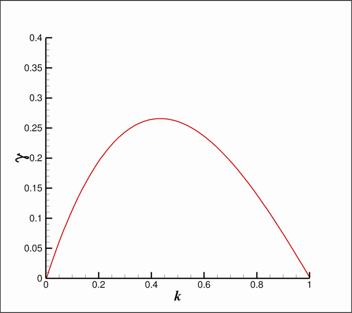
where $\omega$ will be off the real axis as is known for the two-stream instability. We evaluate this $\epsilon$ with the two-stream equilibrium of (66) in order to obtain the linear growth rates. In Appendix A we show that $\epsilon$ can be rewritten in the form

$$\epsilon(z,k)=1-\frac{1}{k^{2}}\left[1-2z^{2}+2Z(z)(z-z^{3})\right]\,,$$ (68)

where $z=\omega/(k\sqrt{2})$ and $Z$ is the usual plasma dispersion function as defined in [34]. Figure 13 is a plot of the growth rate obtained from $\epsilon=0$ adapted to our domain with $L=4\pi$ (cf. [36] Fig. 3) confirming that our early growth is about right.

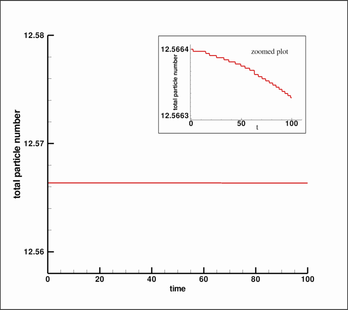
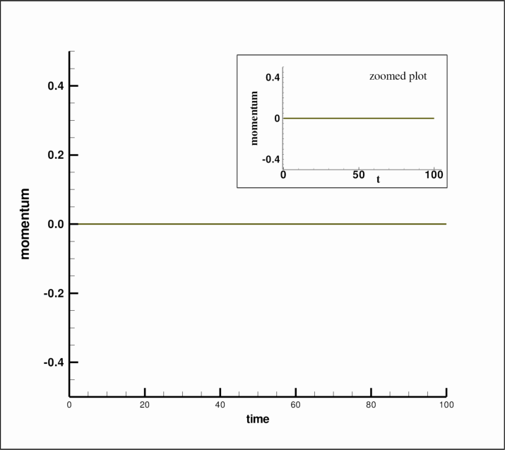
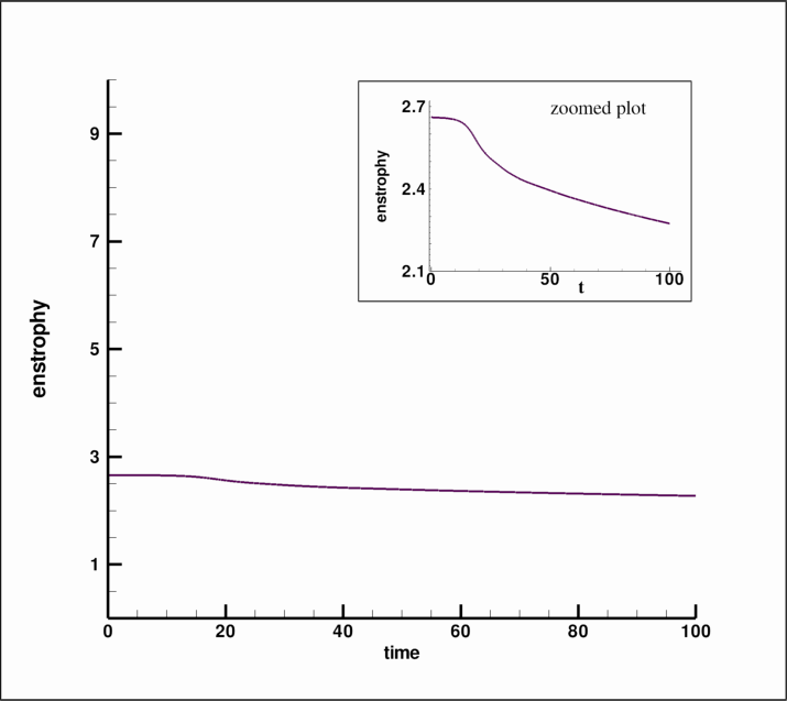
Conservation Properties

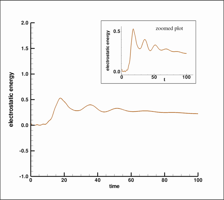
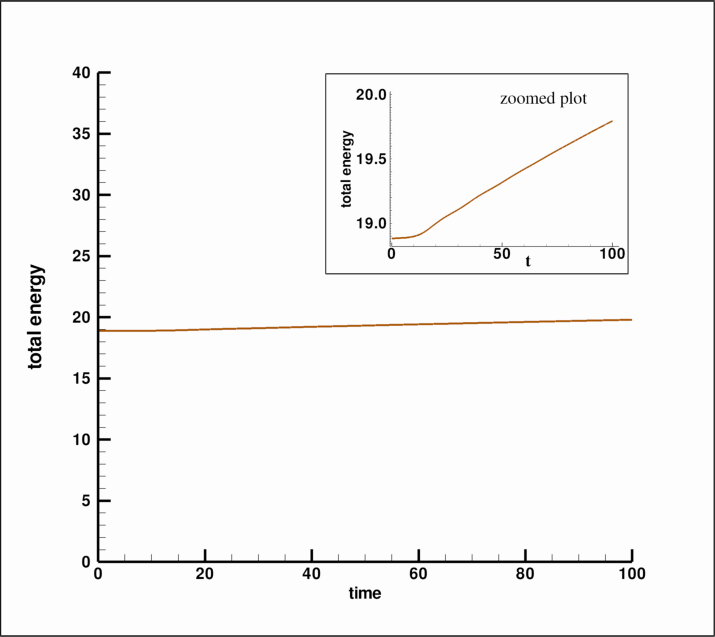
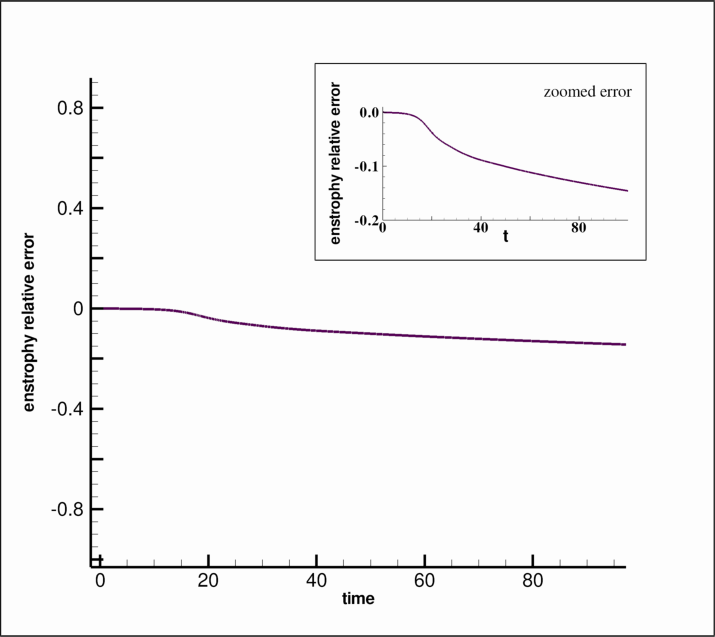
Figure 14 shows plots of the invariants of Section 2 as functions of time, while Fig. 15 depicts the relative error of the total energy, $(H-H_{0})/H_{0}$, and similarly the enstrophy. The top left panel of Fig. 14 shows that the total particle number is conserved quite well, with an error no larger than $0.01\%$ over the full 100 units of time of our simulations. Actually, the DG discretization and Runge-Kutta (RK) method used for time advancement perfectly conserves this quantity for the transport equation. However the nonlinear iteration generates a monotone in time error for the total particle number of order of $10^{-4}$ in 100 time units. The top right panel of Fig. 14 shows the evolution of the total momentum, $P$. This quantity is exactly conserved because the DG method cannot break symmetry, and the same is true for the time advancement algorithm. In fact the method perfectly conserves all odd velocity moments of $f$. The middle left panel of Fig. 14 depicts the evolution of the enstrophy Casimir invariant, $\int dxdvf^{2}$, a q uantity that appears to be seldom-monitored in Vlasov codes ([33] being an exception). From the inset of Fig. 15, it is seen to be conserved to within about 10%, which we suspect is comparatively good, and can be considerably improved by refinement and an increase in polynomial order. Conservation of this quantity arises because the solution of the Vlasov equation is a rearrangement, a property that we discuss below in more detail. It is violated because of small scale error and the diffusive nature of numerical algorithms. Note, like total particle number $N$, the error in the enstrophy is monotonic in time. The middle right and bottom left panels of Fig. 14 show the evolution and error of the kinetic and electrostatic energies (6) and (7), the first and second terms of (10), respectively. Individually these quantitie s are not conserved by the Vlasov equation, as is clearly evident from the figures, but their sum, $H$, shown in the bottom left panel, is conserved with a relative error less than $4\%$ over the entire course of the run. The oscillations in the kinetic and electrostatic energies, indicative of the trapping process, cancel upon addition and give an error that increases monotonically in time. In Fig. 15 the relative error of the enstrophy and total energy are depicted. In other algorithms the error in $H$ is oscillatory in nature, typically with small temporal mean. Even though this mean error could be small, it is important to realize that the oscillations amount, in a sense, to successively reinitializing the code, and the cumulative error of the solution for such a process is hard to assess.

In addition to the conserved quantities of (8), (9), (10), and (11), the Vlasov equation possesses topological conservation. As mentioned above, it is well-known that the solution of the Vlasov equation is a rearrangement [35]. This means that the solution at any time $t$ can be obtained formally from its initial value as follows:

$$f(x,v,t)=f_{0}(x_{0}(x,v,t),v_{0}(x,v,t))=f_{0}\circ z_{0}\,,$$ (69)

where $z_{0}=(x_{0}(x,v,t),v_{0}(x,v,t))$ is obtained upon inverting the solution of the characteristic equations $z=z(z_{0},t)$. Because the characteristic equations have Hamiltonian form they preserve volume (here area), and

$$\frac{\partial(x_{0},v_{0})}{\partial(x,v)}=1\,.$$ (70)

A consequence of this is the family of Casimir invariants of (11), whose invariance follows directly upon effecting the coordinate change $z_{0}\leftrightarrow z$ and making use of (69) and (70):

$$\int dx_{0}\int dv_{0}\,\mathcal{C}(f_{0}(x_{0},v_{0})=\int dx\int dv\,\mathcal{C}(f(x,v,t)\,,$$ (71)

where we have suppressed limits of integration.

Under continuity assumptions, the level sets of $f_{0}$ are topologically equivalent to the composition $f_{0}\circ z_{0}=f$. This is what is meant by topological conservation. It follows that the number and nature of extrema, the values of $f$ at these extrema, and the kinds of separatrices connecting saddle points must correspond to those of $f_{0}$. In addition, although not a topological property, the area between any two contours of $f$ must also be conserved, a consequence of the area preservation property of the characteristics. Since DG is a weak formulation with lack of continuity, the extent to which level sets are actually topologically conserved remains to be seen. Casimir invariants such as enstrophy and entropy may be conserved well and be consistent with rearrangement inequalities such as Jensen’s inequality without the continuity assumption.

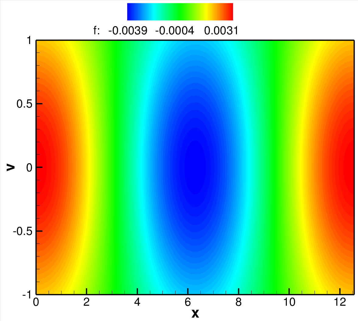
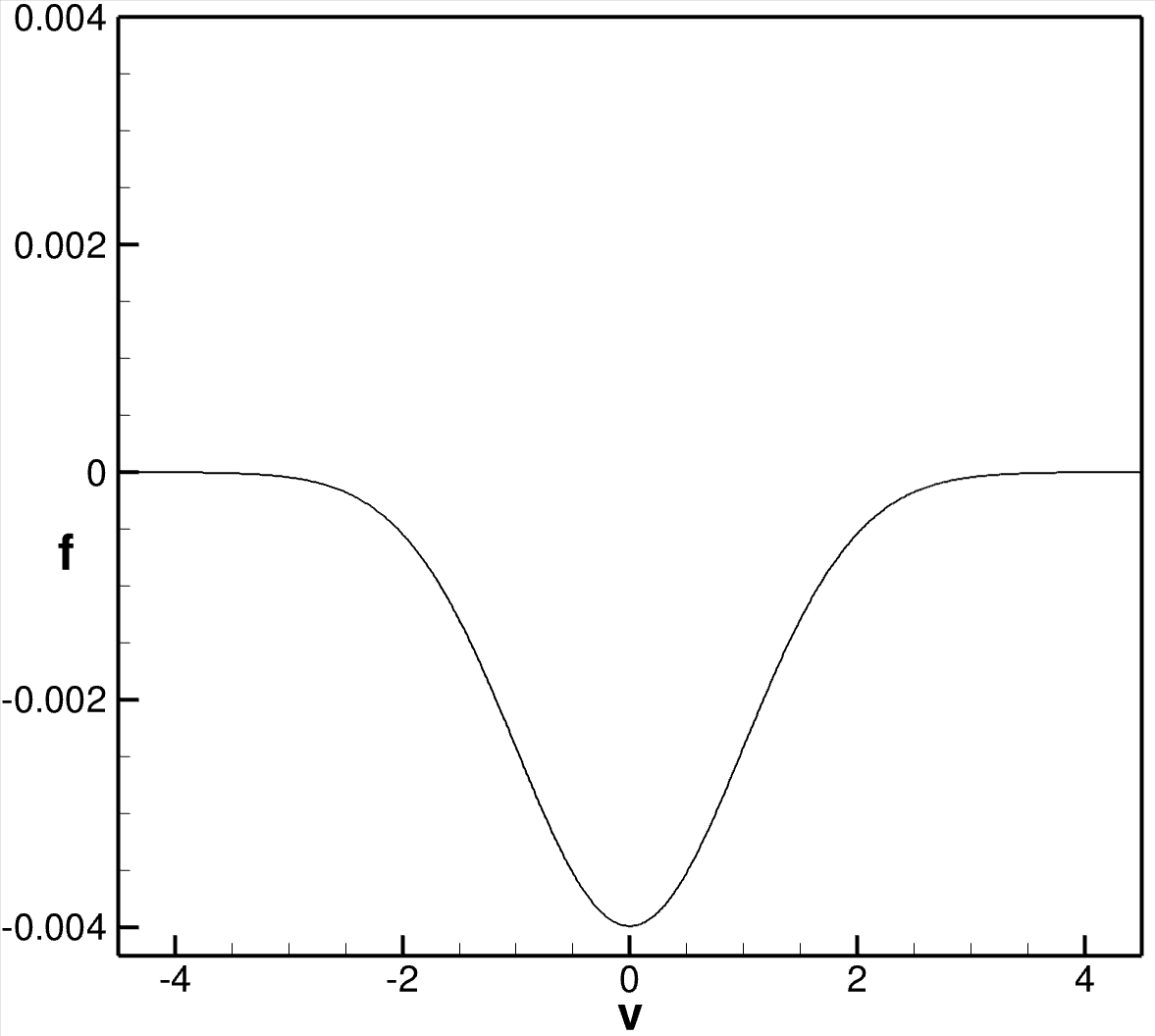
Because the initial condition has the form $f_{0}(x,v)=f_{TS}(v)[1+0.05\cos(x/2)]$, the initial phase space has nearly imperceptible initial ‘tears’ in the first panels of Figs. 10 and 11, that should be consistent with asymptotic state at $t=T=100$. Extrema of $f_{0}(x,v)$ occur at points $(x,v)$: $(x,0)$, for all $x\in\{0,4\pi\}$, $(0,\pm\sqrt{2})$, and $(2\pi,\pm\sqrt{2})$. Thus there is a trough along the line $v=0$. The points $(0,\pm\sqrt{2})=(4\pi,\pm\sqrt{2})$ atop the beams are maxima straddled by thin separatrices entering and emerging from the saddle points located at $(2\pi,\pm\sqrt{2})$. The following extremal values of $f_{0}$ remain fixed in time under Vlasov dynamics, although their locations can change: $f_{0}(0,0)=0$, $f_{0}(2\pi,0)=0$, $f_{0}(0,\pm\sqrt{2})=0.308$, and $f_{0}(2\pi,\pm\sqrt{2})=0.279$. A glance at Fig. 10 shows some degradation of the value of $f$ atop the ridge-like structures, while the vanishing value of $f$ at the points $(0,0)$ and $(2\pi,0)$ is rigorously maintained. A measure of error in an algorithm is the extent to which it fills in the hole, i.e. returns values of $f_{0}(2\pi,0)\neq 0$.

In our simulations the value of $f$ remains zero at the minimum $(2\pi,0)$ and it remains zero to high accuracy at $(0,0)$. The values of $f$ at the extrema and the associated separatrices atop the beams are never very discernible, their existence due to only a few percent in the variation of $f$, and are washed out by numerical dissipation as the contours of the distribution function wrap around and ‘trap particles’ over the course of the simulation. However, the trough at $v=0$ is structurally unstable and separatrices emerge form here and connect the saddle point at $v=0$ and $x=0=4\pi$ that straddles the minimum at $(2\pi,0)$, the center of the electron hole. The eventual boundaries that delineate the trapped and untrapped particle populations, as the potential saturates into what appears to be a final BGK-like state, is what we discuss next.

BGK Saturation

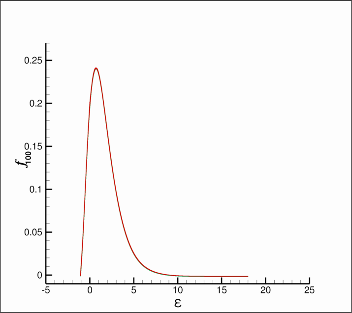
Examination of Figs. 10, 11, and 12 shows the initial linear growth phase, followed by a particle trapping phase, and eventually a strong indication of a saturated state with clean contours of $f$, resulting at least in part from the small scale averaging inherent in any algorithm. It is generally believed that this evolution saturates, in some weak sense, to a BGK mode, although no proof exists. To test this belief we check to see if the contours of $f$ are aligned with contours of the particle energy, $\mathcal{E}=v^{2}/2-\Phi(x,t)$, which is well-known to be the case for an equilibrium state of the Vlasov equation (e.g. [8]).

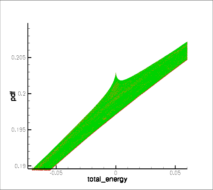
To this end we plot $f_{100}(\mathcal{E}(x,v)):=f(x,v,100)$, where in $\mathcal{E}(x,v)=v^{2}/2-\Phi(x,100)$, the particle energy at $t=100$. (Note, we suppress the time variable.)    Figure 16 clearly indicates that a saturated BGK state has been achieved. Here, in the left panel, we have plotted $f$ versus $\mathcal{E}(x,v)$, at $t=100$, for all 9 million pairs $(x,v)$ of the uniformly distributed mesh over our phase space. Observe that to within the thickness of the line, $f_{100}$ appears as a graph over $\mathcal{E}(x,v)$ and that this is true even for large values of $\mathcal{E}$, where $f_{100}>0$ is maintained. Green and red dots correspond to positive and negative values of the velocity, respectively, and there does not seem to be any systematic directional bias. Because the computation was done for piecewise constant element functions, it is known that DG ensures $f(x,v,t)$ remains positive for all times a nd this is then the case for $f_{100}$. The right panel of Fig. 16 is a plot of the electrostatic potential as a function of position for several instances in time as indicated in the figure. The curve labeled by $t=100$ is taken to be the saturated electrostatic potential that was used in the calculation of $f_{100}$.

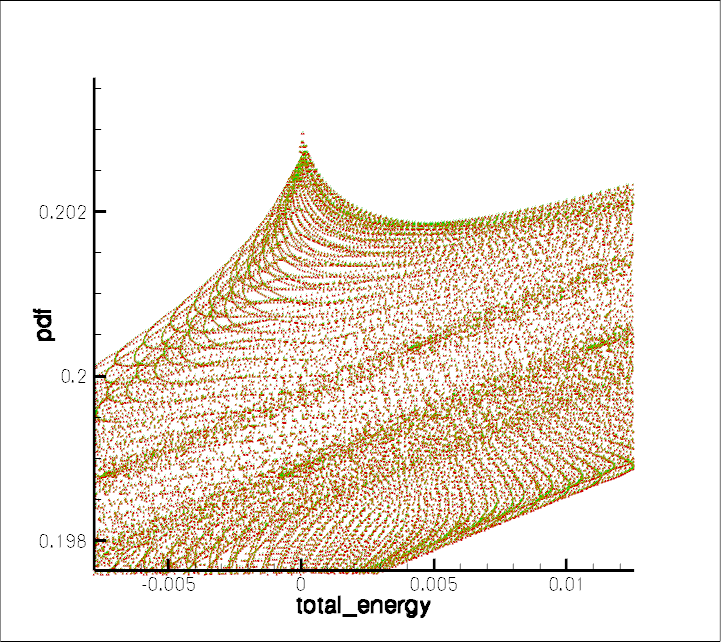
In Figs. 18 and 19 high resolution details of $f_{100}$ are depicted. In Fig. 18 a cusp is seen at the trapping boundary that occurs at $\mathcal{E}=0$. A magnified view of this is shown in Fig. 18. In the course of the evolution the presence of the electrostatic force produces a trapped particle population with $\mathcal{E}<0$. It is conceivable that trapping, like scooping ice cream, is a non-analytic process and that this cusp represents something real about the mathematical nature of the dynamics. However, it also may be attributed to the choice of the numerical scheme, yet discontinuities have previously been proposed at trapping boundaries: in [60] a discontinuity is used in making electron hole models and in [30] two kinds of discontinuities are proposed for adiabatic and sudden trapping. None of these discontinuities match the cusp like feature that we observe, but the traveling wav e state treated in [30] is not the same as that reached by our simulation and it is possible that an analysis similar to that of [30] could produce a cusp. Further studies of this effect are currently being investigated. Figures 18 and 18 examine $f_{100}$ near the minimum value of $\mathcal{E}$. Note the clear steepening of $f_{100}$ as it approaches its minimum value. It is possible that there is a universal nature to both this steepening and to the cusp at the trapping boundary, but we leave an investigation of this to future work. Figures 18 and 18 examine $f_{100}$ near its maximum value. The spread here as well as the other panels of Fig. 18 give a sense of how close the system has relaxed to an equilibrium state.

Figure 19 examines the details of $f_{100}$ for higher values of $\mathcal{E}$. In Fig. 19 a splitting is seen to occur at around $\mathcal{E}=1.3$. In Figs. 19 and 19 we see that this small splitting persists to large values of $\mathcal{E}$. It is interesting to note that because the red and green dots are mixed within each band, the splitting is not an effect of velocity direction. The splitting is within the resolution of the code and is believed to be a real effect, one that seems to indicate that complete saturation has not occurred.

The above tests provide strong indication that the code has relaxed to near a BGK state. As further evidence we test to see if the charge density associated with $f_{100}$ is consistent with that for a final BGK state. To this end we first observe that $f_{100}$ can be fit reasonably well by a model distribution function of the following form:

$$f_{\rm fit}=a(\mathcal{E}+\Phi_{M})(\mathcal{E}+\mathcal{E}^{*})e^{-\beta\mathcal{E}}\,.$$ (72)

Here $\Phi_{M}$ is the maximum value of $\Phi$, and because $\mathcal{E}=v^{2}/2-\Phi$ we see $-\Phi_{M}$ is the smallest possible value of $\mathcal{E}$. This and positivity of $f$ imply $\mathcal{E}^{*}>\Phi_{M}$. Obviously (72) does not account for the fine features discussed above, but it will be sufficient for our purpose.

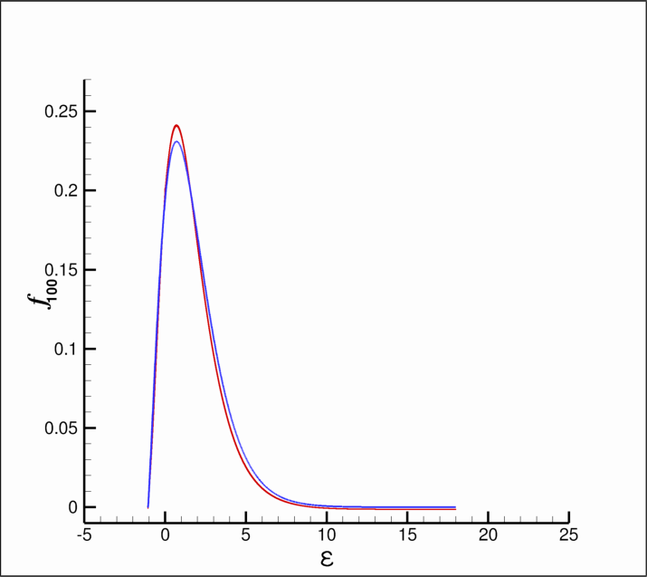
The quantities $a$, $\Phi_{M}$, $\mathcal{E}^{*}$, and $\beta$ are fitting parameters that can be matched to the code output. We obtain a rough idea of the degree of self-consistency, i.e. the degree to which Eq. (72) produces the correct electrostatic potential when substituted into Poisson’s equation, by using the following values extracted from the code output: $\Phi_{M}=1.06$ and $\mathcal{E}^{*}=1.59$. For convenience we choose $\beta=1$. More significant figures in $a$, viz.  $a=0.1148$, are required to ensure that the total net charge is zero. In Fig. 17 we see these choices provide a pretty good fit to the data. However, insufficient charge near the maximum is spread to higher values of $\mathcal{E}$. In a forthcoming publication we will examine this sort of modeling in much greater detail.

We note, there is a relationship between $\mathcal{E}_{M}$, the value at which $f$ obtains its maximum, and the other parameters. That is, $f^{\prime}(\mathcal{E}_{M})=0$ implies

$$\mathcal{E}_{M}=\frac{2-\beta(\Phi_{M}+\mathcal{E}^{*})+\sqrt{4+\beta^{2}(\Phi_{M}-\mathcal{E}^{*})^{2}}}{2\beta}$$ (73)

or

$$\mathcal{E}^{*}=\frac{\Phi_{M}-\beta\mathcal{E}_{M}\Phi_{M}+2\mathcal{E}_{M}-\beta\mathcal{E}_{M}^{2}}{\beta\mathcal{E}_{M}+\beta\Phi_{M}-1}\,,$$ (74)

where the latter is useful when $\mathcal{E}_{M}$ is extracted from data. In fact, the value of $\mathcal{E}^{*}=1.59$ used above follows from $\mathcal{E}_{M}=0.71$ (cf. Fig. 18).

Given $f_{\rm fit}$, the charge density is given by

$$\rho_{\rm fit}(\Phi)=1-\int_{-\infty}^{\infty}\!dv\,f_{\rm fit}=1-\int_{-\Phi}^{\infty}\!\frac{d\mathcal{E}\,f_{\rm fit}(\mathcal{E})}{\sqrt{2(\mathcal{E}+\Phi)}}\,,$$ (75)

where in the second equality the formula $\mathcal{E}=v^{2}/2-\Phi$ is used to change the integration variable from $v$ to $\mathcal{E}$. With the choice (72) this quantity can be explicitly integrated to give

$$\rho_{\rm fit}=1-\frac{\sqrt{2\pi}\,a}{\beta^{5/2}}\left[\frac{3}{4}-\beta^{2}(\Phi_{M}-\Phi)(\Phi-\mathcal{E}^{*})+\frac{\beta}{2}(\Phi_{M}-2\Phi+\mathcal{E}^{*})\right]e^{\beta\Phi}\,.$$ (76)

Defining a pseudopotential $\mathcal{V}$ by $\partial\mathcal{V}/\partial\Phi=\rho_{\rm fit}$, and integrating Poisson’s equation yields

$$\frac{E^{2}}{2}+\mathcal{V}(\Phi)=\mathcal{V}_{0}\,,$$ (77)

where $\mathcal{V}_{0}$ is a constant and

$$\mathcal{V}(\Phi) = \Phi$$

$$- \frac{\sqrt{2\pi}a}{\beta^{7/2}}\left[\frac{15}{4}-\beta^{2}(\Phi_{M}-\Phi)(\Phi-\mathcal{E}^{*})+\frac{3}{2}\beta(\Phi_{M}-2\Phi+\mathcal{E}^{*})\right]\,e^{\beta\Phi}$$

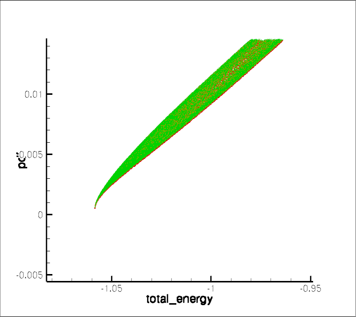
is the expression for the pseudopotential. Here ${E^{2}}/{2}$ acts as a pseudo kinetic energy. Thus we can interpret the BGK state by comparison to a particle dropped in the potential $\mathcal{V}$ at zero kinetic energy. Such a fictitious particle returns to a state of zero kinetic energy as $x$ traverses the spatial domain, which must be the case if there is zero net charge.

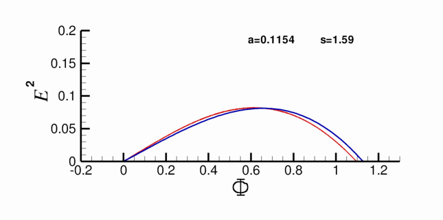
In Fig. 20, $E^{2}$ is plotted against $\Phi$ for our simulation data. In light of (77) and (4.2.2), we expect $E^{2}$ to be a graph over $\Phi$ at time $t=100$, and from the figure this indeed appears to be the case. Also, since at $t=0$, $\Phi^{\prime\prime}=A\cos(x/2)$, it is easy to see that $E^{2}(x,t=0)/2=A\Phi(x,t=0)-\Phi(x,t=0)^{2}/8$. This follows from the choice of ground for $\Phi$ and the absence of net charge which gives via Gauss’ theorem $E(x=4\pi)=E(x=0)$. With our boundary conditions $E(x=0)=0$. Thus we expect the parabolic curve in Fig. 20 labeled by $t=0$ with maximum $\Phi$ occurring $\Phi_{M}=8A=8\times 0.05=0.40$. However, it is remarkable that at intermediate times $E^{2}$ is also a graph over $\Phi$. This can be shown to be true if $\Phi$ maintains symmetry about $x=2\pi$. This suggests that $\Phi$ can serve as a good spatial coordinate, an idea we will discuss further in a forthcoming publication.

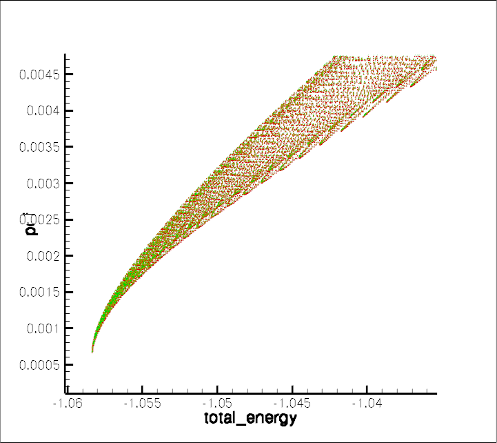
The data of Fig. 20 can be compared to the model of Eq. (77) with (4.2.2). Choosing $\mathcal{V}_{0}$ so that $E^{2}(\Phi=0)=0$ and the parameter values of Fig. 17, yields the plot of Fig.  21. Here we see a reasonable fit to the data at $t=100$. Note, $E^{2}(\Phi_{M})\approx 0$ and the maximum value of $E^{2}$ is a close fit. We note, a certain level of accuracy is needed in the parameters because $E^{2}$ is a sensitive function of $\Phi$. We have not optimized the fit, but the result of Fig. 20 is roughly what one might expect for the expansion of $f_{100}$ with only three terms of a Laguerre series, and thus gives a fair indication of self-consistency which was our goal. As noted above, we will revisit this again in great detail in a future publication.

Figure 10: (Nonlinear two-stream instability) 3D plots of the solution $f$ at $t=0$, $t=20$, $t=40$, $t=60$, $t=80$ and $t=100$.

Figure 11: (Nonlinear two-stream instability) Contour plots of the solution $f$ at $t=0$, $t=20$, $t=40$, $t=60$, $t=80$ and $t=100$.

Figure 12: (Nonlinear two-stream instability) Time series plots of the first four modes: $k=1/2$ (top left), $k=1$ (top right), $k=3/2$ (bottom left), and $k=2$ (bottom right).

Figure 13: Plot of growth rate $\gamma$ vs.  $k$ for the equilibrium distribution function of (66).

Figure 14: (Nonlinear two-stream instability) Temporal evolution of the total particle number $N$ (top left), momentum $P$ (top right), enstrophy (middle left), and kinetic energy (middle right), electrostatic energy (bottom left), and the total energy $H$ (bottom right). See Section 2 for definitions of these quantities.

(a)

(b)

Figure 15: (Nonlinear two-stream instability) Relative error of the enstrophy (left) and the total energy $H$ (right).

.

Figure 16: (Nonlinear two-stream instability) Plot of the distribution function at time $t=100$, $f_{100}$, as a function of the particle energy $\mathcal{E}=v^{2}/2-\Phi(x,t=100)$. Green dots correspond to positive velocities and red dots to negative velocities, $v$ (left). Right panel depicts the potential $\Phi(x,t)$ at the times indicated. $\Phi(x,t=100)$ was used in $\mathcal{E}$ for the plot of $f_{100}$ (right).

Figure 17: (Nonlinear two-stream instability) Model distribution function $f_{\rm fit}$ of Eq. (72) with $\Phi_{M}=1.06$, $\mathcal{E}^{*}=1.59$, $\beta=1$, and $a=0.1148$ (solid blue) compared to code results at $t=100$ (red dots).

Figure 18: (Nonlinear two-stream instability) Fine scale details of the distribution function $f_{100}(\mathcal{E})$, depicting a cusp formation near the trapping boundary at $\mathcal{E}=0$ (top left and right). Near the minimum value of $\mathcal{E}$, $f_{100}$ is observed to greatly steepen (middle left and right). The maximum of $f_{100}$ is achieved at about $\mathcal{E}=0.71$ (bottom left and right). In all plots red dots correspond to negative velocities and green dots to positive velocities, $v$. No asymmetry in the sign of $v$ is evident.

Figure 19: (Nonlinear two-stream instability) Plot of $f_{100}(\mathcal{E})$ near $\mathcal{E}=1.3$ indicating mild splitting (top left), with stronger splitting seen at $\mathcal{E}\approx 1.5$ (top right). The splitting continues to larger values of $\mathcal{E}$ (bottom left and right). Red dots correspond to negative velocities and green dots to positive velocities $v$, with no evident asymmetry in the sign of $v$.

Figure 20: (Nonlinear two-stream instability) Plot of $E^{2}$ versus $\Phi$ for the code output at the times indicated. Note, $E^{2}$ is a graph over $\Phi$ even for the unsaturated states, i.e. times $t\leq 100$.

Figure 21: (Nonlinear two-stream instability) Plot of $E^{2}$ vs. $\Phi$ as given by (77) with (4.2.2) for the model $f_{\rm fit}$ of (72) with the parameters of Fig. 12, and code output (red), both at time $t=100$.

5 Conclusions

In this paper we have demonstrated the viability of the DG method with upwinding for solving the Vlasov-Poisson system. The method was described in detail for general polynomial bases of elements. Several examples were computed to demonstrate the utility of the method using a piecewise uniform basis. A convergence study was performed for the simple advection problem, indicating the degree to which filamentation can be resolved, and high resolution computations of the linearized Vlasov-Poisson system were also performed. For linearization about a Maxwellian equilibrium, computation results were seen to compare very well with theoretical calculations of Landau damping. Computations for Lorentzian equilibria were also presented and the wave number dependence of the Landau damping rate was verified, apparently for the first time in a simulation. The problems of nonlinear Landau damping and the symmetric two-stream instability were then considered, and results were compared to previous calculations. In both cases, constants of motion were monitored and the error was seen to be monotonic, due to nonlinear coupling. Also, reasons for the lack of numerical error in the form of recurrence in our results were discussed. High resolution features of the distribution function were displayed for the long time BGK state that was reached in the two-stream calculations. Comparisons between theory and code results were made, particularly for the end BGK state, in an attempt to provide a high standard for truth in numerical code work.

There are many future directions suggested by this work, some of which are ongoing. In a couple of upcoming publications [18, 17] the authors will report on computations using higher order polynomial bases with an improved temporal integrator and a limiter that maintains positivity of the distribution function, as well as a study of numerical recurrence for these schemes. Indeed, [18] contains a thorough study of dependence of recurrence times and recurrence amplitudes on the mesh size in $x,v$ and the time step $\Delta t$, for Vlasov linear advection, as well as dependence on the order, type, and choice of basis functions for the DG scheme. It is quite remarkable, that for the lowest order polynomial space of piecewice constant functions, one can prove that recurrence occurs, but the recurrence amplitude will decay, thereby suggesting value in choosing lower order functions. This fact significantly improves the performance criteria originally developed in [11].

As noted in the Introduction, the DG method can be run easily on nonuniform meshes, and in work not reported here we have seen this to be the case. This is a first step toward producing an adaptive code. Similarly, parallel implementation awaits. There are many physical applications within reach, such as the treatment of a plasma diode which requires physical boundary conditions and the inclusion of various collision operators of relevance to plasma dynamics. Since the Vlasov-Poisson system serves as a test bed for more sophisticated kinetic theories, it is our opinion that the DG method proposed here is an attractive alternative for many plasma physics computations.

Appendix A Appendix: Dispersion Relations

Here we analyze the dispersion relations for the Lorentzian and two-stream equilibria given by (15) and (66), respectively. With the assumption that $f(x,v,t)=f_{eq}(v)+\delta f(x,v,t)$ and $\delta f(x,v,t)\sim\exp(ikx-i\omega t)$ and the scaling of variables described in Section 2, the plasma ‘dispersion relation’ is given by

$$\epsilon(k,\omega)=1-\frac{1}{k^{2}}\,\int\limits_{-\infty}^{\infty}\frac{f_{eq}^{\prime}(v)}{(v-\omega/k)}\,dv\,,$$ (79)

where $k$ is assumed to be real and positive and for bounded systems $k=2\pi n/L$ with $n$ an integer. Landau damping arises upon analytically continuing this expression into the lower half $\omega$-plane and thus deforming the contour of integration [42]. For integration along the real axis, stable and unstable eigenmodes (and embedded modes if they exist) satisfy

$$\epsilon(k,\omega)=0\,,$$ (80)

and it is this quantity we wish to investigate for both discrete modes and Landau ‘modes’, the latter obtained by analytic continuation into the lower half $\omega$-plane. In the latter case, the solution $\omega(k)$ of (80) characterizes the asymptotic-time behavior of mode $E_{k}(\omega,t)$ of the electric field. Specifically, if $\omega=\omega_{R}+i\gamma$, where $\omega_{R}$ and $\gamma$ are real-valued, then $\gamma<0$ is the time-asymptotic rate of decay of the mode $E_{k}(\omega,t)$ and $\omega_{R}$ is the frequency of oscillation.

For the Lorentz equilibrium distribution function of (15),

$$f_{eq}^{\prime}(v)=-\frac{2}{\pi}\,\frac{v}{(v^{2}+1)}\ .$$ (81)

Upon defining $u=\omega/k$ and substituting (81) into (79), we obtain

$$\epsilon(k,ku)=1+\frac{2}{\pi k^{2}}\,\int_{-\infty}^{\infty}\frac{v}{(v^{2}+1)^{2}(v-u)}\,dv\,,$$ (82)

which expresses $\epsilon$ as a function $u$ and $k$. Evaluation of this integral is a straightforward application of Cauchy’s theorem. Assuming $u$ is in the upper half plane, poles exist at $v=i$ and $v=u$, with corresponding residues of the integrand being $R_{i}=i/[4(u-i)^{2}]$ and $R_{u}=u/(u^{2}+1)^{2}$. Summing over the residues gives the dispersion function

$$\epsilon(k,ku)=1-\frac{1}{k^{2}(u+i)^{2}}\,.$$ (83)

Upon setting $\epsilon=0$, since $\omega=ku$, we obtain

$$\omega=\pm 1-ik=\omega_{R}+i\gamma\,,$$ (84)

which demonstrates, contrary to our assumption, that there are no discrete modes in the upper half $u$-plane. This is consistent with the well-known result that equilibrium distribution functions that are monotonic in $v^{2}$ possess no discrete growing or damped modes. However, continuing (83) into the lower half plane gives Landau damping with $\gamma(k)=-k$ and $|\omega_{R}(k)|=1$ for the time asymptotic behavior.

For the two-stream equilibrium of (66), (79) gives rise to instability, i.e., for this case there is in fact a root with $u$ in the upper half plane. For computational reasons it is convenient to write $\epsilon$ in terms of the plasma $Z$-function which is related to both the Hilbert transform and the error function (see e.g. [34]). Upon inserting (66) and performing some manipulation, (79) can be written as

$$\epsilon=1-\frac{2}{k^{2}}\left[J_{1}(z)+J_{2}(z)\right]\,,$$ (85)

where

$$J_{1}(z)=\frac{1}{\sqrt{\pi}}\int_{-\infty}^{\infty}e^{-w^{2}}\frac{w\,dw}{w-z}\,,\quad\quad J_{2}(z)=\frac{1}{\sqrt{\pi}}\int_{-\infty}^{\infty}e^{-w^{2}}\frac{w^{3}\,dw}{w-z}\,,$$ (86)

and $z=u/\sqrt{2}$. With the standard definition of the plasma $Z$-function,

$$Z(z)=\frac{1}{\sqrt{\pi}}\int_{-\infty}^{\infty}e^{-w^{2}}\frac{dw}{w-z}=2ie^{-z^{2}}\int_{-\infty}^{iz}e^{-t^{2}}dt$$ (87)

where in the first expression $\Im(z)>0$ and the value of $Z$ for $\Im(z)<0$ is obtained by analytic continuation, while the second expression is valid for all complex $z$. The second expression is desirable for computations. Also, sometimes it is convenient to use the derivative formula

$$Z^{\prime}=-2(1+zZ)\,,$$ (88)

which is valid for all $z$. After some more-or-less standard manipulations and making use of (88), we obtain

$$\epsilon=1-\frac{2}{k^{2}}\left[1-2z^{2}+2zZ(z)\left(1-z^{2}\right)\right]\,.$$ (89)

We numerically evaluated this expression and searched for its roots to obtain Fig. 13. Because our system has the size $L=4\pi$, we write $\epsilon(k,\omega)$ with $k$ replaced by $k/2$.

References

- [1] B. Ayuso, J. A. Carrillo, C.-W. Shu, Discontinuous Galerkin methods for the one-dimensional Vlasov-Poisson system, Preprint UAB. (2010).
- [2] B. Ayuso de Dios, J. A. Carrillo, C.-W. Shu, Discontinuous Galerkin methods for the multi-dimensional Vlasov-Poisson problem, Preprint UAB. (2010).
- [3] T. P. Armstrong, R. C. Harding, G. Knorr, and D. Montgomery, Solution of Vlasov’s equation by transform methods, Methods in Computational Physics, 9, 29-86 (1970).
- [4] I. Babuška, The finite element method with Lagrangian multipliers, Numerische Mathematik, 20, 179-192 (1973).
- [5] I. Babuška, The finite element method with penalty, Mathematics of Computation, 27, 221-228 (1973).
- [6] I. Babuška and M. Zlámal, Nonconforming elements in the finite element method with penalty, SIAM Journal on Numerical Analysis, 10, 863-875 (1973).
- [7] R. Balescu Statistical mechanics of charged particles (Wiley-Interscience, New York, 1963).
- [8] I. B. Bernstein, J. M. Greene, and M. D. Kruskal, Exact nonlinear plasma oscillations, Phys. Rev. 108, 546-550 (1957).
- [9] C. K. Birdsall and A. B. Langdon, Plasma physics via computer simulation (Institute of Physics Publishing, Bristol/Philadelphia, 1991).
- [10] F. F. Chen, Introduction to plasma physics and controlled fusion (Plenum Press, New York, 1984).
- [11] C. Z. Cheng and G. Knorr, The integration of the Vlasov equation in configuration space, Journal of Computational Physics, 22, 330-351 (1976).
- [12] Y. Cheng, I. M. Gamba, A. Majorana and C.-W. Shu, Discontinuous Galerkin solver for the semiconductor Boltzmann equation, in Simulations of Semiconductor Processes and Devices, Vol. 12, (Eds. T. Grasser and S. Selberherr) (Springer, Wien, 2007) pp. 257-260.
- [13] Y. Cheng, I. M. Gamba, A. Majorana, and C.-W. Shu, Discontinuous Galerkin solver for Boltzmann-Poisson transients, Journal of Computational Electronics, 7, 119-123 (2008).
- [14] Y. Cheng, I. M. Gamba, A. Majorana, and C.-W. Shu, A discontinuous Galerkin solver for Boltzmann Poisson systems in nano devices, Comput. Methods Appl. Mech. Engrg., 198, 3130-3150 (2009).
- [15] Y. Cheng, I. M. Gamba, A. Majorana, and C.-W. Shu, A discontinuous Galerkin solver for full-band Boltzmann-Poisson models, in 13th International Workshop on Computational Electronics Proceedings, 211-214 (2009).
- [16] Y. Cheng, I. M. Gamba, A. Majorana, and C.-W. Shu, Discontinuous Galerkin methods for the Boltzmann-Poisson systems in semiconductor device simulations AIP Conference Proceedings Volume 1333, ISBN: 978-0-7354-0889-0 , pp 890-895 (2010).
- [17] Y. Cheng, I. M. Gamba, Numerical study of Vlasov-Poisson equations in the simulation for infinite homogeneous stellar systems. To Appear in Communications in Nonlinear Science and Numerical Simulation, (2011).
- [18] Y. Cheng, I. M. Gamba, and P. J. Morrison, On Runge-Kutta discontinuous Galerkin schemes for Vlasov-Poisson systems, preprint (2011).
- [19] Y. Cheng, I. M. Gamba, Fengyan Li and P. J. Morrison, High order positive discontinuous Galerkin schemes for Maxwell-Vlasov systems, in preparation, (2011).
- [20] Y. Cheng, I. M. Gamba and J. Proft, Positive and stable discontinuous Galerkin schemes for linear Vlasov-Boltzmann transport equations, to appear in Mathematics of Computation, (2011).
- [21] B. Cockburn and C. N. Dawson, Some extensions of the local discontinuous Galerkin method for convection-diffusion equations, The Proceedings of the Conference on the Mathematics of Finite Elements and Applications, Elsevier, 225-238 (2000).
- [22] B. Cockburn, S. Hou, and C. W. Shu, The Runge-Kutta local projection discontinuous Galerkin finite element method for conservation laws IV: the multidimensional case, Mathematics of Computation, 54, 545-581 (1990).
- [23] B. Cockburn, S. Y. Lin, and C. W. Shu, TVB Runge-Kutta local projection discontinuous Galerkin finite element method for conservation laws III: one-dimensional systems, Journal of Computational Physics, 84, 90-113 (1989).
- [24] B. Cockburn and C. W. Shu, TVB Runge-Kutta local projection discontinuous Galerkin finite element method for conservation laws II: general framework, Mathematics of Computation, 52, 411-435 (1989).
- [25] B. Cockburn and C. W. Shu, The local discontinuous Galerkin method for time-dependent convection-diffusion systems, SIAM Journal on Numerical Analysis, 35, 2440-2463 (1998).
- [26] J. Canosa, J. Gazdag, and J. E. Fromm, The recurrence of the initial state in the numerical solution of the Vlasov equation, Journal of Computational Physics, 15, 34–45 (1974).
- [27] J. M. Dawson, Particle simulation of plasmas, Reviews of Modern Physics, 55, 403-447 (1983).
- [28] C. Dawson, S. Sun, and M. F. Wheeler, Compatible algorithms for coupled flow and transport, Computer Methods in Applied Mechanics and Engineering, 193, 2565-2580 (2004).
- [29] J. Denavit and W. L. Kruer, Comparison of numerical solutions of the Vlasov equation with particle simulations of collisionless plasmas, Phys. Fluids 14, 1782-1791 (1971).
- [30] R. L. Dewar, Frequency shift due to trapped particles, Phys. Fluids 15, 712-714 (1972).
- [31] B. Eliasson, Outflow boundary conditions for the Fourier transformed one-dimensional Vlasov-Poisson system, Journal of Scientific Computing, 16,1–28 (2001).
- [32] L. C. Evans, Partial differential equations (American Mathematical Society, Providence, Rhode Island, 1998).
- [33] F. Filbet, E. Sonnendrücker, and P. Bertrand, Conservative numerical schemes for the Vlasov equation, Journal of Computational Physics, 172, 166-187 (2001).
- [34] B. D. Fried and S. D. Conte, The plasma dispersion function (Academic, London, 1961).
- [35] C. S. Gardner, Bound on the energy available from a plasma, Phys. Fluids 6, 839–840 (1963).
- [36] F. C. Grant and M. R. Feix, Fourier-Hermite solutions of the Vlasov equations in the linearized limit, Phys. Fluids 10, 696-702 (1967).
- [37] R. E. Heath, Numerical analysis of the discontinuous Galerkin method applied to plasma physics Ph.D. dissertation, The University of Texas at Austin, Austin, 2007. Available at: http://repositories.lib.utexas.edu/ bitstream/handle/2152/3065/heathr64379.pdf. (Note, this thesis contains a few typographical errors, but the intent is clear.)
- [38] R. W. Hockney and J. W. Eastwood, Computer simulation using particles (McGraw-Hill, New York, 1981).
- [39] M. G. Kivelson and C. T. Russel, Introduction to space physics (Cambridge University Press, Cambridge, 1996) pp. 37-38.
- [40] A. J. Klimas, A numerical method based on the Fourier-Fourier transform approach for modeling 1-D electron plasma evolution, Journal of Computational Physics, 50, 270-306 (1983).
- [41] A. J. Klimas and W. M. Farrell, A splitting algorithm for Vlasov simulation with filamentation filtration, Journal of Computational Physics, 110, 150-163 (1994).
- [42] L. D. Landau, On the vibrations of the electronic plasma, Journal of Physics U.S.S.R., 10, 25, 25-34 (1946).
- [43] P. LeSaint and P. A. Raviart, On a finite element method for solving the neutron transport equation, Mathematical Aspects of Finite Elements in Partial Differential Equations, 89-123 (1974).
- [44] E. M. Lifshitz and L. P. Pitaevskii, Physical kinetics: Course of theoretical physics Vol. 10 ( Pergamon Press, Oxford, 1981). Translated from Russian by J. B. Sykes and R. N. Franklin.
- [45] A. Mangeney, F. Califano, C. Cavazzoni, and P. Trávníc̆ek, A numerical scheme for the integration of the Vlasov-Maxwell system of equations, J. Comp. Phys., 179, 495-538 (2002).
- [46] V. P. Maslov and M. V. Fedoryuk, The linear theory of Landau damping, Mathematics of the USSR-Sbornik, 55, 2, 437-465 (1986).
- [47] N. P. Meredith, R. B. Horne, R. H. A. Iles, R. M. Thorne, D. Heynderickx, and R. R. Anderson, Outer zone relativistic electron acceleration associated with substorm-enhanced whistler mode chorus, J. Geophys. Res., 107, A7, 1144 (2001).
- [48] D. C. Montgomery and D. A. Tidman, Plasma kinetic theory (McGraw-Hill, New York, 1964).
- [49] P. J. Morrison, The Maxwell-Vlasov equations as a continuous Hamiltonian system, Phys. Lett. 80A, 383-386 (1980).
- [50] P. J. Morrison, Poisson brackets for fluids and plasmas, in Mathematical Methods in Hydrodynamics and Integrability in Dynamical Systems, eds. M. Tabor and Y. Treve, American Institute of Physics Conference Proceedings No. 88, New York (1982) pp. 13–46.
- [51] P. J. Morrison and D. Pfirsch, Dielectric energy versus plasma energy, and Hamiltonian action-angle variables for the Vlasov equation, Phys. Fluids 4B, 3038–3057 (1992).
- [52] P. J. Morrison, Hamiltonian description of Vlasov dynamics: action-angle variables for the continuous spectrum, Transport Theory and Statistical Physics 29, 397–414 (2000).
- [53] C. Mouhot and C. Villani, On Landau damping, arXiv:0904.2760. To appear in Acta Mathematica (2011).
- [54] T. Nakamura and T. Yabe, Cubic interpolated propagation scheme for solving the hyper-dimensional Vlasov-Poisson equation in phase space, Computer Physics Communications, 120, 122-154 (1999).
- [55] J. A. Nitsche, Über ein Variationsprinzip zur Lösung von Dirichletproblemen bei Verwendung von Teilräumen, die keinen Randbedingun-gen unterworfen sind, Anh. Math. Sem. Universität Hamburg, 36, 9-15 (1971).
- [56] E. Pohn, M. Shoucri, and G. Kamelander, Eulerian Vlasov codes, Computer Physics Communications, 166, 181-93 (2005).
- [57] T. R. Reed and W. H. Hill, Triangular mesh methods for the neutron transport equation, LA-UR-73-479, Los Alamos Scientific Laboratory, Los Alamos, NM (1973).
- [58] G. Rein, Collisionless kinetic equations from astrophysics - the Vlasov-Poisson system, in Handbook of Differential Equations, Evolutionary Equations, Vol. 3, (Eds. C. M. Dafermos and E. Feireisl), (Elsevier, 2007).
- [59] B. Riviere, M. F. Wheeler, and V. Girault, A priori error estimates for finite elements based on discontinuous approximation spaces for elliptic problems, SIAM Journal on Numerical Analysis, 39, 902-931 (2001).
- [60] H. Schamel, Electron holes, ion holes and double layers, Phys. Repts. 140, 161-191 (1986).
- [61] M. Shoucri, The method of characteristics for the solution of hyperbolic differential equations, Computer Physics Research Trends, (Nova Science, 2007), 1-82.
- [62] E. M. Stein and G. Weiss, Introduction to Fourier analysis on Euclidean spaces (Princeton University Press, Princeton, NJ, 1971).
- [63] S. Sun, Discontinuous Galerkin methods for reactive transport in porous media (Ph.D. dissertation, The University of Texas at Austin, Austin, 2003).
- [64] S. Sun and M. F. Wheeler, Symmetric and nonsymmetric discontinuous Galerkin methods for reactive transport in porous media, SIAM Journal on Numerical Analysis, 43, 195-219 (2005).
- [65] F. Valentini, Nonlinear Landau damping in nonextensive statistics, Phys. Plasmas, 12, 072106 (2005).
- [66] F. Valentini, and R. D’Agnosta, Electrostatic Landau pole for -velocity distributions, Phys. Plasmas, 14, 092111 (2007).
- [67] F. Valentini, P. Trávníc̆ek, F. Califano, P. Hellinger, and A. Mangeney, A hybrid-Vlasov model based on the current advance method for the simulation of collisionless magnetized plasma, J. Comp. Phys., 225, 753-770 (2007).
- [68] F. Valentini, P. Veltri, and A. Mangeney, A numerical scheme for the integration of the Vlasov-Poisson system of equations, in the magnetized case, J. Comp. Phys., 210, 730-751 (2005).
- [69] N. G. Van Kampen, On the theory of stationary waves in plasmas, Physica, 21, 949-963 (1955).
- [70] M. F. Wheeler, An elliptic collocation-finite element method with interior penalties, SIAM Journal on Numerical Analysis, 15, 152-161 (1978).
- [71] M. F. Wheeler and P. Percell, A local residual finite element procedure for elliptic equations, SIAM Journal on Numerical Analysis, 15, 705-714 (1978).
- [72] S. I. Zaki, L. R. T. Gardner, and T. J. .M. Boyd, A finite element code for the simulation of one-dimensional Vlasov plasmas. I. Theory, Journal of Computational Physics, 79, 184-199 (1988).
- [73] S. I. Zaki, L. R. T. Gardner, and T. J. .M. Boyd, A finite element code for the simulation of one-dimensional Vlasov plasmas. II. Applications, Journal of Computational Physics, 79, 200-208 (1988).
- [74] Q. Zhang and C. W. Shu, Stability analysis and a priori error estimates to the third order explicit Runge-Kutta discontinuous Galerkin Method for scalar conservation laws, SIAM J. Numer. Anal. 48 (2), 772-795 (2010).
- [75] Q. Zhang and C. W. Shu, On maximum-principle-satisfying high order schemes for scalar conservation laws, J. Comput. Phys.229 3091-3120, (2010).
- [76] T. Zhou, Y. Guo, and C. W. Shu, Numerical study on Landau damping, Physica D, 157, 322-333 (2001).