Power Euclidean metrics for covariance matrices with application to diffusion tensor imaging
Abstract
Various metrics for comparing diffusion tensors have been recently proposed in the literature. We consider a broad family of metrics which is indexed by a single power parameter. A likelihood-based procedure is developed for choosing the most appropriate metric from the family for a given dataset at hand. The approach is analogous to using the Box-Cox transformation that is frequently investigated in regression analysis. The methodology is illustrated with a simulation study and an application to a real dataset of diffusion tensor images of canine hearts.
Keywords: Box-Cox transformation, diffusion tensor, Euclidean, Fréchet mean, likelihood, log-Euclidean, positive demi-definite, Procrustes analysis.
1 Introduction
In many applications it is of interest to consider statistical analysis of covariance matrices. In particular, typical tasks might be to estimate a mean covariance matrix, describe the structure of the variability in the matrices, and interpolate between covariance matrices. A key aspect of such analysis is the choice of metric for comparing covariance matrices.
In medical imaging a particular type of data structure commonly arises when analysing diffusion weighted images, called the diffusion tensor (Basser et al., 1994; Alexander, 2005). The diffusion tensor (DT) is simply a positive semi-definite symmetric matrix which is related to the covariance matrix of the diffusion of water molecules at a particular voxel in the brain. In diffusion tensor imaging a number of different metrics have been proposed for comparing two tensors , which are symmetric positive semi-definite covariance matrices. Metrics include the Euclidean metric, Riemannian metric (Pennec et al., 2006), log-Euclidean metric (Arsigny et al., 2007), Cholesky metric (Wang et al., 2004), and the Procrustes size-and-shape metric (Dryden et al., 2009), among many others. In several of these papers it has been demonstrated how the choice of metric makes a substantial difference to estimation and interpolation. However, for a particular application at hand, which is the preferred choice of metric?
Statistical approaches to the analysis of DT data include Schwartzman et al. (2010), Whitcher et al. (2007), Zhu et al. (2007, 2009), and, for example, hypothesis tests for group means and extensions of regression models are considered. However, the choice of statistical model or metric on the space of diffusion tensors is problem specific.
The aim of this paper is to consider a family of metrics indexed by a single power parameter. We will develop likelihood-based methods for estimation of the power parameter, which will enable us to select the most appropriate metric from the family. The methodology is applied to simulated data and a real dataset of diffusion tensors from a sample of canine hearts. The procedure that is developed is directly analogous to the use of variance stabilizing Box-Cox transformations that are very commonly used in regression analysis in statistics (Box and Cox, 1964). The general idea is that a suitable metric for a problem will be based on a power transformation that makes the data “as Gaussian as possible”.
2 Power Euclidean metrics
2.1 Metrics and the sample Fréchet mean
Let be the usual spectral decomposition with an orthogonal matrix and diagonal with strictly positive entries. Let be a diagonal matrix with logarithm of the diagonal elements of on the diagonal. The logarithm of is given by and likewise the exponential of the matrix is . The log-Euclidean metric (Arsigny et al., 2007) is given by
| (1) |
A broad family of covariance matrix metrics is the set of power Euclidean metrics
| (2) |
where (see Dryden et al., 2009). As the metric approaches the log-Euclidean metric of (1). We could consider any depending on the situation, and we use the log-Euclidean metric if . Note that all these metrics are Euclidean metrics, with curvature of the space being zero. Tangent space co-ordinates are also therefore very simple. If the covariance matrices must be strictly positive definite, but if then we can compare positive semi-definite matrices.
Consider a random sample available from a population. The sample Fréchet mean based on metric is calculated by finding
In our case with all the power metrics, the manifold is isomorphic to a convex subset of , and the existence and uniqueness of the mean follows immediately (Karcher, 1977; Le, 1995).
The sample Fréchet mean of the powered covariance matrices provides an estimate of the population covariance matrix, and is given by
For the estimators become more resistant to outliers for smaller , and for larger the the estimators become less resistant to outliers. For one is working with powers of the inverse covariance matrix. The resulting fractional anisotropy measure using the power metric (2) is given by
and . A practical visualisation tool is to vary in order for a neurologist to help interpret the white fibre tracts in the images (Dryden et al., 2009).
A question of interest is what should we take in practice? We develop a criterion which involves choosing to make the data as multivariate Gaussian as possible, as statistical inference should be more straightforward in such cases. Such a criterion is similar to the Box-Cox transformation used in regression analysis, except in our case we are working with matrix powers of symmetric positive definite matrices.
2.2 Likelihood
First of all we write down the probability density function for , , which is assumed to be multivariate Gaussian in the distinct elements of . The density of is
where the parameters are (a vector) and (a symmetric positive definite matrix). Note that is a vector of the elements in the upper triangle of .
Our data though are given as , so we transform from to using , to give the density of . The transformation can be carried out in three stages. We first transform from to , where is the usual spectral decomposition with and is diagonal with positive, distinct diagonal values. We then transform from to and then finally we transform to . Using Fang and Zhang (1990, p24) the Jacobian of the first transformation is given by
where and is the first -dimensional principal minor of . The second transformation has Jacobian
and finally the third transformation has Jacobian
Putting these togther the density of given is:
Hence, given a random sample of diffusion tensors the log-likelihood of the parameters is given by
| (3) |
2.3 Statistical Inference
Maximum likelihood estimation of the parameters in the model is straightforward if is known, in which case and are given by the usual Gaussian m.l.e.s of the sample mean and sample covariance matrices of , where .
Hence, a method for estimation is to evaluate the profile log-likelihood for a range of (substituting in the maximum likelihood estimators (m.l.e.’s) of given ). The Jacobian term is straightforward to evaluate if the eigenvalues of are sufficiently distinct. However, if some of them are close to each other then a Taylor series expansion is used for numerical evaluation. Also, a Taylor series expansion is used for close to zero. In particular, writing then we have the Taylor Series expansion
which can be used for computation when the eigenvalues become close. Also, the Taylor series expansion in terms of is
which is useful for small .
In order to obtain confidence intervals for we use Wilks’ Theorem which states that, for large samples,
where is the likelihood ratio for testing versus . In practice, an approximate 95% confidence interval is obtained by the values of which have log-likelihood within from the maximum.
3 Applications
3.1 Simulation study
We initially consider a simulation study with and are simulated from a multivariate Gaussian
and then the symmetric matrix is transformed to the matrix . A random sample of matrices are simulated for voxels, with samples at each voxel. Each of the simulated tensors are independent and identically distributed. We consider an example simulation where the true mean matrix is , the true and is the noise variance.
For each simulated sample of size the m.l.e. and confidence intervals for are obtained, by evaluating the log-likelihood over a range of values for . In our example the range of values for evaluation is in steps of . The m.l.e. of maximizes the log-likelihood (3), and the confidence interval is taken as the range of within of the maximum of the log-likelihood.
From Monte Carlo simulations we count the number of times that the true lies inside the estimated confidence interval. The results are given in Table 1. We see that the coverage is low for small samples, with the confidence intervals being conservative. However, coverage is very good for here.
INSERT TABLE 1 ABOUT HERE
3.2 Canine Hearts
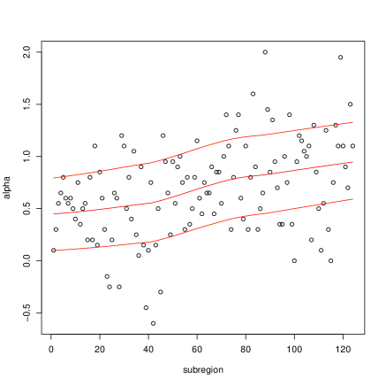
The estimation of and confidence intervals are also carried out for data on a subset of registered DT images of canine hearts. The dataset consists of nine registered hearts, and is described by Peyrat et al. (2007). There are DT images which have been registered and then a mask is extracted. We take an equally spaced grid at intervals of mm in the mask and consider a neighbourhood of voxels within a ball of radius mm. We consider interior points where the sub-region contains at neighbourhood voxels in addition to the voxel itself (where ). Hence, we have voxels contributing to the likelihood of (3), with a common and . The parameter is estimated by maximum likelihood using the voxels in each local sub-region. Hence, we are able to estimate in different regions of the heart.
We consider analysis of the DT data using a global normalization (as the data have been measured at different temperatures) and also without normalization. The DTs have been normalised for each heart by taking an overall mean tensor (using Euclidean mean ) and then dividing by the norm of this average matrix.
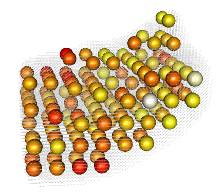
The results of the canine hearts analysis for the normalized data are displayed in Figures 1 and 2. We see that is generally lower on the left of this region and higher on the right. Values are particularly high at the upper right in the view in Figure 2. In practice one would wish to use the procedure to choose a single value of suitable for the whole image, perhaps rounded to the nearest half for ease of explanation. Regarding the smoother estimates of Figure 1 values of in the range would not be unreasonable for this dataset, hence a suitable rounded choice would be , corresponding to the matrix square root.
INSERT FIGURES 1 AND 2 ABOUT HERE
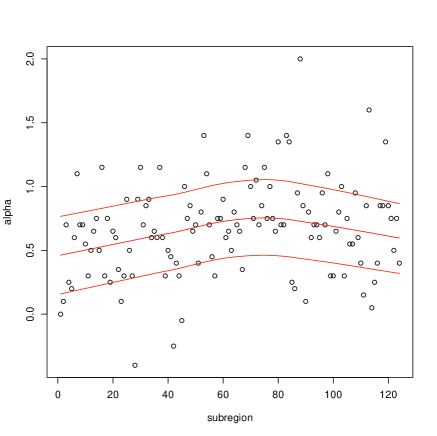
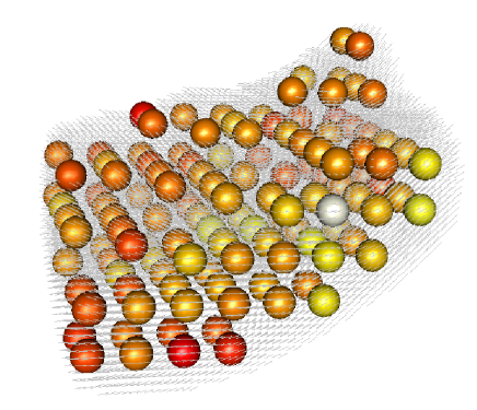
In Figures 3-4 we see the equivalent plots for the non-normalized data. Again values in the range seem reasonable, although there is no longer a pattern of general increase from left to right. Rather the larger values are at the front/middle of the subregion. On average the estimates are a little lower than for the normalized data, but an overall rounded value of would be reasonable for these data as well.
INSERT FIGURES 3 AND 4 ABOUT HERE
Once a suitable value of has been estimated then statistical analysis of the diffusion tensors can proceed. For example, we may wish to consider mean diffusion tensors in a region using the Fréchet mean, we might want to carry out interpolation in space between tensors or alternatively consider fibre tracking using the metric corresponding to the estimated .
4 Further work
Rather than working with the symmetric power matrices, we could match two power matrices closer by post multiplying by an orthogonal matrix:
| (4) |
Note that is symmetric, but is not symmetric in general. The motivation for carrying out this additional matching is that we can decompose as
where , and so the covariance matrix is invariant to the choice of . The Euclidean power metric involves fixing , with symmetric. The Procrustes solution for matching to is , where are obtained from a singular value decomposition:
and is a diagonal matrix of singular values. The resulting metric is equivalent to Kendall’s Riemannian size-and-shape metric in the size-and-shape space of points in dimensions (see Dryden et al., 2009, when ). This non-Euclidean space has positive curvature, and is a cone with a warped product metric (Kendall, 1989; Dryden and Mardia, 1998). However, for practical use and in some simulation studies the Proctustes metric and the Euclidean power metric often perform similarly (see Dryden et al., 2009 in the case). Further properties and practical usage of the Procrustes power metric will be investigated in further work.
From the application point of view, more experimental data would be need to clearly establish what is the best metric for inter-subject comparison. It would also be very interesting to compare with the optimal metric for the intra-subject measurement noise. This last metric could be estimated from repeated scan of the same subject.
Acknowledgements
Funding for this work was provided in part by the Leverhulme Trust.
References
- [Alexander, 2005] Alexander, D. C. (2005). Multiple-fiber reconstruction algorithms for diffusion MRI. Ann NY Acad Sci, 1064:113–133.
- [Arsigny et al., 2007] Arsigny, V., Fillard, P., Pennec, X., and Ayache, N. (2007). Geometric means in a novel vector space structure on symmetric positive-definite matrices. SIAM Journal on Matrix Analysis and Applications, 29(1):328–347.
- [Basser et al., 1994] Basser, P. J., Mattiello, J., and Le Bihan, D. (1994). Estimation of the effective self-diffusion tensor from the NMR spin echo. J Magn Reson B., 103:247–254.
- [Box and Cox, 1964] Box, G. E. P. and Cox, D. R. (1964). An analysis of transformations. (With discussion). J. Roy. Statist. Soc. Ser. B, 26:211–252.
- [Dryden et al., 2009] Dryden, I. L., Koloydenko, A., and Zhou, D. (2009). Non-euclidean statistics for covariance matrices, with applications to diffusion tensor imaging. Annals of Applied Statistics, 3:1102–1123.
- [Dryden and Mardia, 1998] Dryden, I. L. and Mardia, K. V. (1998). Statistical Shape Analysis. Wiley, Chichester.
- [Fang and Zhang, 1990] Fang, K.-T. and Zhang, Y.-T. (1990). Generalized multivariate analysis. Springer, Berlin.
- [Karcher, 1977] Karcher, H. (1977). Riemannian center of mass and mollifier smoothing. Comm. Pure Appl. Math., 30(5):509–541.
- [Kendall, 1989] Kendall, D. G. (1989). A survey of the statistical theory of shape (with discussion). Statistical Science, 4:87–120.
- [Le, 1995] Le, H.-L. (1995). Mean size-and-shapes and mean shapes: a geometric point of view. Advances in Applied Probability, 27:44–55.
- [Pennec et al., 2006] Pennec, X., Fillard, P., and Ayache, N. (2006). A Riemannian framework for tensor computing. Int. J. Comput. Vision, 66(1):41–66.
- [Peyrat et al., 2007] Peyrat, J.-M., Sermesant, M., Pennec, X., Delingette, H., Xu, C., McVeigh, E. R., and Ayache, N. (2007). A computational framework for the statistical analysis of cardiac diffusion tensors: Application to a small database of canine hearts. IEEE Transactions on Medical Imaging, 26(11):1500–1514.
- [Schwartzman et al., 2010] Schwartzman, A., Dougherty, R. F., and Taylor, J. E. (2010). Group comparison of eigenvalues and eigenvectors of diffusion tensors. Journal of the American Statistical Association, 105:588–599.
- [Wang et al., 2004] Wang, Z., Vemuri, B., Chen, Y., and Mareci, T. (2004). A constrained variational principle for direct estimation and smoothing of the diffusion tensor field from complex DWI. IEEE Trans. on Medical Imaging, 23(8):930–939.
- [Whitcher et al., 2007] Whitcher, B., Wisco, J. J., Hadjikhani, N., and Tuch, D. S. (2007). Statistical group comparison of diffusion tensors via multivariate hypothesis testing. Magn. Reson. Med., 57:1065–1074.
- [Zhu et al., 2009] Zhu, H., Cheng, Y., Ibrahim, J. G., Li, Y., Hall, C., and Lin, W. (2009). Intrinsic regression models for positive-definite matrices with applications to diffusion tensor imaging. Journal of the American Statistical Association, 104:1203–1212.
- [Zhu et al., 2007] Zhu, H., Zhang, H., Ibrahim, J. G., and Peterson, B. S. (2007). Statistical analysis of diffusion tensors in diffusion-weighted magnetic resonance imaging data. Journal of the American Statistical Association, 102:1085–1102.
| Monte Carlo Coverage () | ||
|---|---|---|