Abstract

We imaged comet 10P/Tempel 2 on 32 nights from 1999 April through 2000 March. R-band lightcurves were obtained on 11 of these nights from 1999 April through 1999 June, prior to both the onset of significant coma activity and perihelion. Phasing of the data yields a double-peaked lightcurve and indicates a nucleus rotational period of 8.941 $\pm$ 0.002 hr with a peak-to-peak amplitude of $\sim$0.75 mag. Our data are sufficient to rule out all other possible double-peaked solutions as well as the single- and triple- peaked solutions. This rotation period agrees with one of five possible solutions found in post-perihelion data from 1994 by Mueller and Ferrin (1996, Icarus, 123, 463–477), and unambiguously eliminates their remaining four solutions. We applied our same techniques to published lightcurves from 1988 which were obtained at an equivalent orbital position and viewing geometry as in 1999. We found a rotation period of 8.932 $\pm$ 0.001 hr in 1988, consistent with the findings of previous authors and incompatible with our 1999 solution. This reveals that Tempel 2 spun-down by $\sim$32 s between 1988 and 1999 (two intervening perihelion passages). If the spin-down is due to a systematic torque, then the rotation period prior to perihelion during the 2010 apparition is expected to be an additional 32 s longer than in 1999.

Keywords: comets: general – comets: individual (10P/Tempel 2) – methods: data analysis – techniques: photometric

1 Introduction

Comet 10P/Tempel 2 was discovered by E.W.L. Tempel on 1873 July 4. It was recovered in 1878, but not during the 1883 or 1889 apparitions. It has been observed on every return since 1894 except three (1910, 1935, and 1941) when it was particularly poorly placed for observing (Kronk, 2003, 2007, 2009). While telescopic improvements now allow it to be observed at every apparition, the roughly 5.5 year period results in apparitions which alternate between favorable and unfavorable viewing geometries. Consequently, Tempel 2 was well placed for observing in 1978, 1988, and 1999, but poorly placed in 1983, 1994, and 2004 when it reached perihelion on the far side of the Sun.

Tempel 2 was extensively observed during its favorable 1988 return. Because it is only weakly active until shortly before perihelion (Sekanina (1979) and references therein), a nucleus lightcurve can be measured. This allowed a number of investigators to measure the rotation period. The earliest results came from Jewitt & Meech (1988) who found likely periods of 8.9 $\pm$ 0.1 hr or 7.5 $\pm$ 0.1 hr. Jewitt & Luu (1989) extended these observations to near perihelion, concluding that the rotation period was 8.95 $\pm$ 0.01 hr. Comparable periods were determined by A’Hearn et al. (1989) (8.9 hr) and Wisniewski (1990) (8.93 hr). Sekanina (1991) combined these data to determine a sidereal period of 8.93200 $\pm$ 0.00006 hr.

Mueller & Ferrin (1996) observed Tempel 2 for three nights 7–9 months after perihelion in 1994, after coma activity had subsided. Their rotation coverage was insufficient to determine a unique period solution, and they found five possible periods due to aliasing: 8.877 hr, 8.908 hr, 8.939 hr, 8.971 hr, and 9.002 hr. All of these periods were incompatible with the 1988 data, and they concluded that “the period is definitely different between the 1988 and the 1994 apparitions.” Because of aliasing, it was not known if Tempel 2 had spun-up or spun-down since 1988, merely that its rotation period had changed.

The idea of comet rotation periods changing due to outgassing dates to Whipple (1950) and his icy conglomerate model of the nucleus, with various authors since then arguing for spin-up or spin-down (see Samarasinha et al. (2004) for a thorough review). Numerical modeling has shown that, depending on the initial conditions, either spin-up or spin-down is possible, with sustained outgassing over many orbits leading to spin-up and ultimately nucleus splitting (Samarasinha & Belton, 1995; Neishtadt et al., 2002; Gutiérrez et al., 2003). Measurement of a change in the rotation period of a comet, combined with detailed knowledge of the spin axis orientation, nucleus size and shape, and the outgassing rate can constrain the bulk density and internal structure. Due to the difficulty of studying comet nuclei directly, these properties are only well known for a handful of comets, mostly the result of spacecraft visits.

While simulations have shown that changes in rotation period should be common, a strong case can be made for a changing rotation period in only a few comets: 10P/Tempel 2 (sign of the change unknown prior to this work; Mueller & Ferrin (1996)), 2P/Encke (spin-up; Fernández et al. (2005)), 9P/Tempel 1 (spin-up; Belton & Drahus (2007); Chesley et al. (2010)), and Comet Levy (1990c = C/1990 K1; spin-up; Schleicher et al. (1991); Feldman et al. (1992)). The paucity of clear detections of this phenomenon is probably due to the difficulty of obtaining high quality datasets of the same comet over multiple apparitions. By combining our extensive data obtained during the 1999 apparition with those of previous authors from 1987–1988 and 1994, this work will show that 10P/Tempel 2 is the first comet known to spin-down.

We observed Tempel 2 from 1999 April until 2000 March, obtaining images in broadband and narrowband optical wavelengths. Observations prior to perihelion (1999 September 8) were primarily obtained with a broadband R filter to measure the nucleus lightcurve. Once activity began in earnest, observations were primarily obtained with narrowband comet filters (Farnham et al., 2000) to study coma morphology. In this paper, we consider only the pre-perihelion nucleus lightcurve in order to resolve the ambiguity about the sign of the change in rotation period and to conclusively demonstrate that Tempel 2 has spun-down since 1988. A second paper (Paper 2) is planned and will utilize data obtained during 2010 in concert with data obtained during the active phase of the 1999 apparition to determine the pole orientation and the location of any active areas.

The layout of the paper is as follows. We summarize our observing campaign and data reductions in Section 2. In Section 3 we analyze the data, determine the rotation period, compare it with earlier datasets, and consider the effects of viewing geometry, coma contamination, and the lightcurve asymmetry. Finally, in Section 4 we discuss the implications of our results and make predictions for the 2010 apparition.

2 Observations and Reductions

2.1 Observing Overview

We obtained images of Tempel 2 on a total of 32 nights between 1999 April and 2000 March, with sampling at monthly or shorter intervals. For the study presented here, we use only the data obtained from 1999 April through 1999 June, with the dates and observing circumstances listed in Table 1. Additional pre-perihelion data were obtained on 1999 July 10, July 16, August 4, August 5, and September 2. However, these nights all had poor weather and the data were unusable for the present study. By 1999 October, the observing window was very short and the comet had extensive coma contamination, making a period determination challenging.

The April and May observations were obtained at the Lowell Observatory Perkins 1.8-m telescope with the SITe 2K CCD. On-chip 4$\times$4 binning of the images produced a pixel scale of 0.61 arcsec. The June observations were obtained at the Hall 1.1-m telescope with the TI 800 CCD. On-chip 2$\times$2 binning produced images with a pixel scale of 0.71 arcsec. At various times during these runs, we used broadband Kron-Cousins V and R filters and the HB narrowband comet filters (Farnham et al., 2000). However, as planned, only the R filter measurements are extensive enough for the lightcurve analysis discussed here, so we limit this study to those data. Comet images were guided at the comet’s rate of motion. The comet showed evidence of a coma throughout the apparition, progressively increasing with time (see Section 2.4).

2.2 Reductions

The data were reduced using standard bias and flat field techniques. Landolt standard stars (Landolt, 1992) were observed to determine the instrumental magnitude and extinction coefficients on 1999 June 8–11. We observed HB narrowband standard stars (Farnham et al., 2000) on all photometric nights, and used these stars as a bootstrap to estimate absolute R-band calibrations for the photometric nights on which Landolt standard stars were not observed.

Fluxes were extracted by centroiding on the nucleus and integrating inside circular apertures, with the median sky calculated in an annulus centered on the nucleus with inner and outer radii $\sim$33 and $\sim$40 arcsec, respectively. By extracting fluxes through a series of circular apertures (3, 6, 9,…30 arcsec radius), we monitored the lightcurve for incursion from passing stars which show up in the larger apertures earlier than the smaller apertures. The 6 arcsec radius aperture gave the most coherent lightcurve and was used for photometric analysis; this was selected to be large enough to include most of the light from the nucleus even when the seeing was poor and the nucleus PSF was large, while avoiding as much contamination from passing stars as possible.

In order to produce usable lightcurves from non-photometric nights, we applied extinction corrections and the absolute calibrations from photometric nights with the same telescope and instrument configuration. Thus, we applied the absolute calibrations from April 19 to April 17–18 and May 26–27, and the calibrations from June 23 to June 22. The deviation of the brightness from photometric nights helps give an estimate of how much obscuration was affecting the non-photometric nights. Field stars on each image were monitored on non-photometric nights to adjust the comet’s magnitude for varying obscuration during the night (discussed in the following subsection).

2.3 Comparison Star Corrections

Relative photometry of the comet with respect to field stars was carried out. However, not enough of the same field stars were available during the entire night and we therefore replaced stars which left the field of view with new ones as they entered. When possible we used only stars brighter than m_R = 15, but if fewer than three were available, we used fainter stars, going as faint as m_R = 16. Typically between three and six comparison stars were available at a given time.

Reliable catalog magnitudes were not available for enough comparison stars to use comparison stars for absolute calibrations. Therefore, we first used the median of the seven brightest measurements for a given star during the night as its least obscured brightness and determined the adjustment necessary to bring all fainter measurements into agreement. The comparison star correction for an image was the median offset from each star’s least obscured brightness during the night for all comparison stars on a given image. Magnitude corrections derived from comparison stars were applied on the nights specified as non-photometric in Table 1. No comparison star corrections were applied for the photometric nights after first using the comparison stars to confirm that the nights were indeed photometric. Nightly median comparison star corrections were 0.1–0.4 mag, although some corrections exceeded 1.0 mag on 1999 April 18.

Since the least obscured brightness of the field stars will be fainter than their ideal brightness if it had been photometric, this technique will introduce a systematic nightly magnitude offset from night to night. Therefore, after correcting the relative photometry with field stars, the entire lightcurve for each night was adjusted so that the peaks for all nights of data were at the same magnitude ($\Delta$m₂, discussed in Section 2.5). If the conditions varied during a night such that there was less obscuration while certain stars were observed but more obscuration while other stars were observed, the uncertainty in the comparison star correction will increase. Hence, the lightcurves on non-photometric nights may exhibit more scatter.

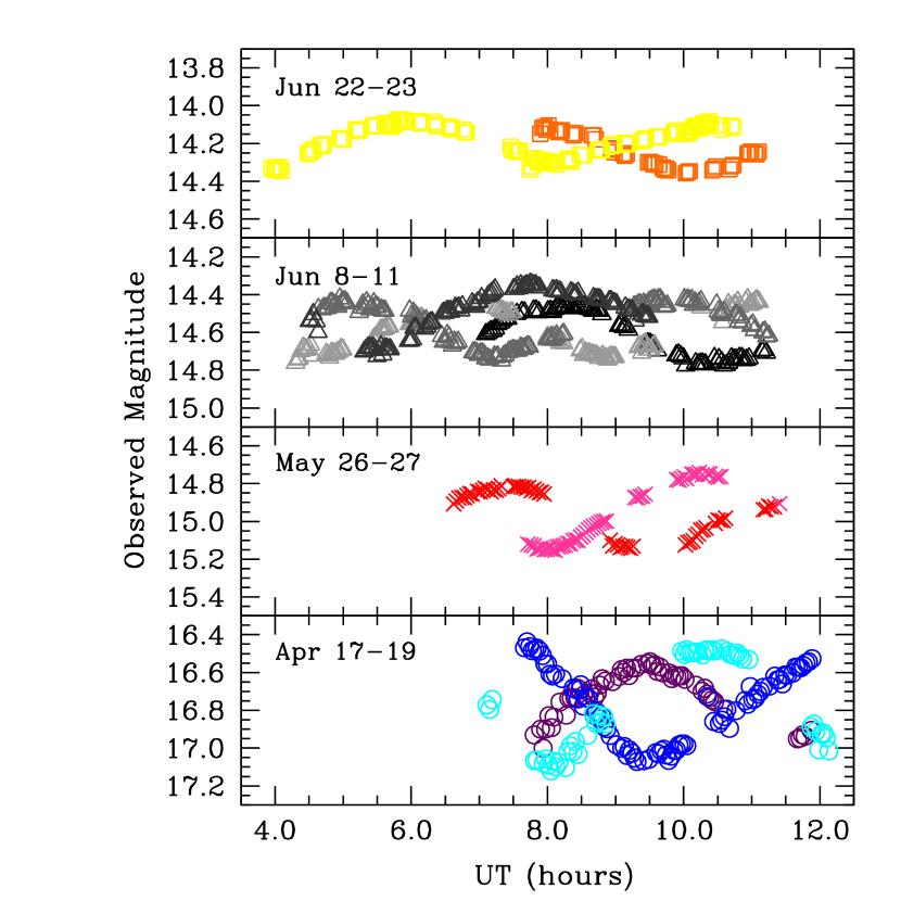
Figure 1: Observed R-band magnitudes (m_R) for our 1999 data plotted as a function of UT on each night. The magnitudes have had absolute calibrations, extinction corrections, and comparison star corrections applied and are given in column (3) of Table LABEL:t:photometry. Starting with the bottom panel and moving up, the first panel (circles) displays April 17 (purple), April 18 (blue), and April 19 (cyan). The second panel (crosses) displays May 26 (red) and May 27 (pink). The third panel (triangles) displays June 8 (black), June 9 (light gray), June 10 (medium gray), and June 11 (dark gray). The top panel (squares) displays June 22 (orange) and June 23 (yellow). Note that throughout the time of interest, decreasing $r$ and $\Delta$ caused the comet to brighten while at the same time increasing coma damped out the amplitude variations of the nucleus. Thus the range of magnitudes is different in each panel, although the vertical scale is held constant at 1 mag to emphasize the decreased amplitude.

The calibrated, extinction corrected, and comparison star corrected R magnitudes (m_R) are plotted in Figure 1 as a function of UT. This indicates how much nightly coverage was obtained. In April and May, Tempel 2 was observed for about five hours, while in June it was observed for about seven hours, with the observing window moving earlier each night. Because the comet brightened during the apparition and the coma increased, the median magnitude is different in each figure and later nights have smaller amplitudes (the vertical scale is held fixed in all panels but the range of magnitudes varies from panel to panel). In order to create a uniform dataset for period analysis and to study the lightcurve amplitudes, we removed the coma, corrected for changing $r$, $\Delta$, and $\phi$, and adjusted for nightly offsets. These adjustments will be discussed in the next two sections.

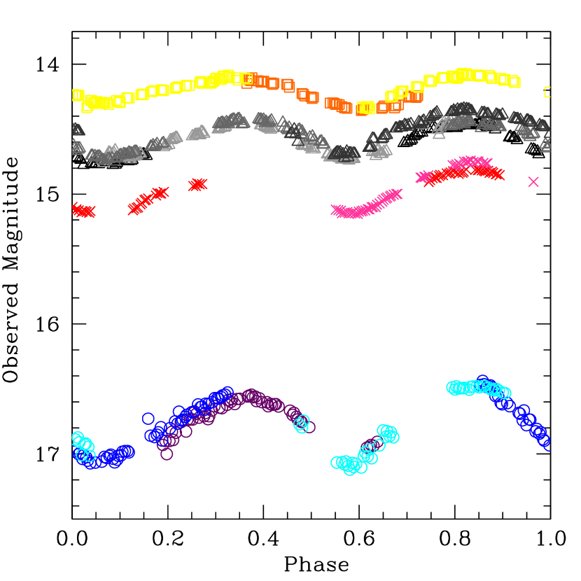
Figure 2: Observed R-band magnitudes (m_R) for our 1999 data phased to our best period of 8.941 hr (discussed in Section 3.1). The magnitudes have had absolute calibrations, extinction corrections, and comparison star corrections applied and are given in column (3) of Table LABEL:t:photometry. Zero phase was set at perihelion (1999 September 8.424). The points are as given in Figure 1. Note that throughout the time of interest, decreasing $r$ and $\Delta$ caused the comet to brighten while at the same time increasing coma damped out the amplitude variations of the nucleus. This figure illustrates the phase coverage obtained during each run, and shows that the lightcurves could be phased even without removing coma contamination.

In Figure 2 we show the same data as in Figure 1 but phased to 8.941 hr (our best period which will be discussed in Section 3.1). This figure emphasizes the increase in brightness and decrease in amplitude throughout the run, as later nights are higher in the figure and have smaller amplitudes. It also demonstrates the phase coverage obtained during each run, making it possible to determine the rotation period even without removing the coma contamination.

2.4 Removal of Coma Contamination

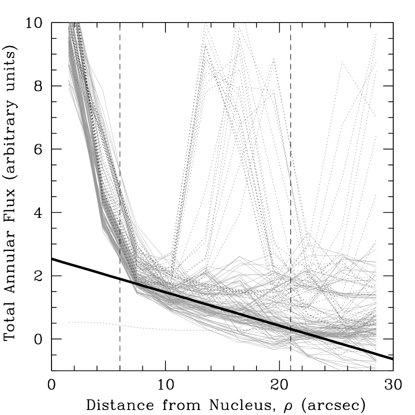
Figure 3: Representative nightly radial profile (1999 June 9). Each curve is composed of the total annular flux (in arbitrary units) in 3 arcsec wide annuli. The solid light gray curves are the radial profiles for images which were used to estimate a nightly median coma profile. The dotted dark gray curves are the radial profiles for images which had contamination by background stars and were not used to determine the nightly median coma profile. The heavy black curve is the nightly median coma profile. This was determined by taking the median of all the light gray curves at the midpoint of each annulus, then fitting a straight line to this nightly radial profile for annuli between 6–21 arcsec (the vertical dashed lines), and extrapolating the fit in to the nucleus and out to 30 arcsec. If the coma decreased as $\rho$^-1 the coma profile would be a horizontal line. The coma profile was never a horizontal line due to the wings of the nucleus PSF, contamination from background stars, and possibly a non-$\rho$^-1 fall off of the coma. We fit a straight line as a first order approximation. Higher order fits varied more from image to image. See the text for further discussion.

While Tempel 2 is not strongly active, some coma was visible throughout the apparition. The coma contamination is, in general, not large and the rotation period can be determined without coma removal. However, to ensure that it was not affecting our results and to compare the amplitude of the lightcurve with those obtained by other authors, we removed the coma inside the monitoring aperture. For unchanging grains flowing radially outward from the nucleus at a constant velocity, the coma flux per pixel decreases as $\rho$^-1, where $\rho$ is the projected distance from the nucleus. Since the area of equally spaced annuli increases as $\rho$, the total coma flux in each annulus should be constant. In reality, the coma often does not fall off as $\rho$^-1 and there are factors which may cause further deviation from a constant total flux per annulus such as contamination by background stars or cosmic rays, wings of the nucleus PSF, and imperfect background removal. However, we found that a linear fit to the total annular flux as a function of annular distance from the nucleus ($\rho$) provides a reasonable first order approximation of the coma. This is illustrated in Figure 3 using 1999 June 9 as a representative night.

We calculated the total flux in 3 arcsec wide annuli centered on the nucleus (e.g., 0–3 arcsec, 3–6 arcsec,…27–30 arcsec) to create radial profiles (total annular flux as a function of $\rho$) for each image. These are plotted as solid light gray curves (images without significant contamination from background stars) and dotted dark gray curves (images with significant contamination from background stars) in Figure 3. We then computed the median total flux in each annulus for the night, ignoring images with obvious contamination from background stars. Next, we fit a straight line to the total annular flux as a function of distance from the nucleus, $\rho$, (the heavy black line in Figure 3) from $\rho$ = 7.5–19.5 arcsec for each image (where $\rho$ = 7.5 arcsec was the center of the 6–9 arcsec annulus and $\rho$ = 19.5 arcsec was the center of the 18–21 arcsec annulus). This range was chosen to exclude as much of the signal from the nucleus ($\rho<$ 6 arcsec) as possible and to minimize contamination from passing stars ($\rho>$ 21 arcsec). We extrapolated the fit in to the nucleus ($\rho$ = 0 arcsec) and out to $\rho$ = 30 arcsec. The total coma annular flux was removed from the total annular flux to give the coma corrected total annular flux (i.e. the total nucleus annular flux), which was integrated and converted back to magnitudes. Since the monitoring aperture was 6 arcsec in radius, the total coma which was removed for a night was the sum of the total coma annular flux in the 0–3 and 3–6 arcsec radius annuli.

When determining the nightly coma, we excluded images with stars which obviously altered the fit. Stars that contaminate the larger annuli tend to result in an under-removal of coma in the monitoring aperture, while stars closer to the nucleus tend to result in an over-removal of the coma in the monitoring aperture. While we excluded the images with obvious contamination from background stars, fainter stars undoubtedly remain. Since more background stars pass through the larger annuli than the smaller annuli, this results in a systematic under-removal of the coma.

As shown in Figure 3, typical profiles appear to have some curvature. This implies that more coma should be removed than is accomplished with a linear fit. A significant contributor to the curvature at small $\rho$ is likely the wings of the nucleus PSF, while at large $\rho$, the coma signal may simply be too small and is swamped by uncertainty in the background removal. We considered higher order fits to better match the curvature; a quadratic fit removed 20–60% more coma while an exponential fit was poor as it often implied negative nucleus counts. Although these fits removed more coma than the linear fit, they varied more from image to image, resulting in wider variance in the estimated coma. Also, small fluctuations in the larger annuli, where there is very little coma, have a large effect on the estimate of the coma contamination for these fits. Therefore, we concluded that a simple linear fit provided the best compromise for approximating the coma profile. We note that if a different fit to the coma were used, it would somewhat alter the amplitude of the lightcurve but would not change the location of its extrema. Thus, the coma removal technique does not affect the key result of this paper, the period determination (Section 3.1).

To test that our use of a single nightly coma correction was appropriate, we determined linear coma fits for each usable image on a night. We saw no systematic variation in the estimated coma flux within the photometric aperture as a function of rotational phase throughout the entire campaign, confirming that the use of a single nightly median correction was reasonable. As another test of the coma removal technique, we investigated the total annular nucleus flux remaining after coma removal. The median fraction for all nights of the nucleus flux contained in the 3 arcsec radius aperture relative to the 9 arcsec radius aperture was 85%. The median for the 6 arcsec radius aperture relative to the 9 arcsec radius aperture was 99%. Apertures larger than 9 arcsec in radius were within $\pm$1% of the 9 arcsec radius aperture flux before deviating at $\rho$ $>$ 21 arcsec (which was beyond the range of the coma fit). These ratios were relatively constant throughout the apparition. The ratio of the 3 arcsec radius aperture relative to the 9 arcsec radius aperture varied with seeing changes, but the 6 arcsec radius aperture did not change appreciably. This confirms that the 6 arcsec radius aperture is appropriate for photometric monitoring, and that the light lost by not going to larger apertures should be minimal and roughly the same fraction in all images, causing no effect on the amplitude of the lightcurve, regardless of seeing.

2.5 Magnitude Adjustments

The viewing circumstances changed significantly during our observations. Therefore, we adjusted the nucleus magnitudes using the standard asteroidal normalization

$$m_{R}(1,1,0)=m_{R,cr}-5log(r\Delta)-\beta\alpha$$ (1)

where m_R(1,1,0) is the normalized magnitude at $r$ = $\Delta$ = 1 AU and $\alpha$ = 0^∘, m_R,cr is the apparent magnitude, m_R (which has had the absolute calibrations, extinction corrections, and comparison star corrections applied), with the coma removed, $r$ is the heliocentric distance (in AU), $\Delta$ is the geocentric distance (in AU), $\beta$ is the linear phase coefficient, and $\alpha$ is the phase angle. $\beta$ is typically 0.03–0.04 mag deg^-1 for comets, and we used $\beta$ = 0.032 mag deg^-1 since it minimized the $\Delta$m₂ adjustment (discussed in the following paragraph). Equation 1 removes the secular variation in brightness and allows comparison of all lightcurves on a similar scale. The geometric corrections are given as $\Delta$m₁ in column (11) in Table 1 at the midpoint of each night’s observations.

The geometric corrections do not always bring the lightcurves from different nights to the same peak brightness, with variations as high as 0.33 mag. This is due to a number of factors, including: bootstrapping Landolt standard stars from HB standards on photometric nights when Landolt stars were not observed; the application of absolute calibrations on non-photometric nights; comparison stars that are normalized to their brightest point in the night rather than a catalog value; and the shape of the coma removed. Therefore, we introduced an additional adjustment, $\Delta$m₂ (column (12) in Table 1), to adjust the individual lightcurves to a common peak brightness. It should be noted that this factor is introduced to simplify the rotation period analysis, and should not be interpreted as representing any particular physical property.

After phasing the data with preliminary $\Delta$m₂ values, we refined $\Delta$m₂ so that all lightcurves were aligned at the peak near $\sim$0.85 phase when possible. April 17 and June 22 were aligned using the peak near $\sim$0.35 phase. Since April 18 and June 9 did not have conclusive peaks, $\Delta$m₂ for these nights was estimated based on the cluster of points near phase 0.85.

2.6 Data

The photometry is given in Table LABEL:t:photometry. Columns (1) and (2) are the UT date and time (at the telescope) at the midpoint of each exposure (adjustments for light travel time are given in Table 1). Column (3) is m_R, the observed R-band magnitude after photometric calibrations, extinction corrections, and comparison star corrections have been applied. Column (4) is m_R^∗, the coma-removed, reduced magnitude m_R(1,1,0) corrected by $\Delta$m₂ so that all nights have a similar peak magnitude. We obtained 1016 data points, of which 124 were discarded due to contamination from background stars, tracking problems, or cosmic ray hits.

While there are several adjustments which have been applied to arrive at the m_R^∗ values listed in Table LABEL:t:photometry, they do not affect the primary focus of the paper: the rotation period determination. The corrections for geometry ($\Delta$m₁) and nightly offsets ($\Delta$m₂) shift individual nightly lightcurves up or down, but the locations of the extrema in rotational phase do not change. While the choice of coma removal algorithm affects the amplitude of the lightcurve, it also leaves the phase of the extrema unchanged. Therefore, the same rotation period could be determined directly from the m_R values prior to the corrections.

Due to the large number of sources of error for each data point (photon uncertainty in comet and background flux, extinction correction, comparison star correction, coma removal), we estimated the effective uncertainty in the magnitude by fitting a smoothed spline through each night’s lightcurve and subtracting the spline fit. The uncertainty for the night was estimated as the standard deviation of the residuals. The uncertainty was not always constant throughout a night since seeing conditions and obscuration varied on the non-photometric nights, so on some nights we estimated the uncertainty for subsections of the lightcurve. Variations in the comparison star magnitudes were used as an additional indicator of when the uncertainty changed during a night. The range of uncertainties for a night are given in column (11) in Table 1.

3 Modeling and Interpretation

3.1 Determining the Rotation Period in 1999

We defined zero phase to be perihelion (1999 September 8.424), and accounted for the light travel time (column (8) in Table 1) before phasing the data. We used an interactive period search routine within the Data Desk data analysis package which updates the phased lightcurves on the fly, allowing us to easily scan through potential periods. We looked for alignment of extrema since they can be identified in phase space even if the magnitudes or amplitudes are different. As the correct solution is approached, the extrema tend to be systematically shifted in phase based on the (color-coded) date of observation, making it easy to quickly hone in on the optimal solution. However, it is difficult to quantitatively estimate the uncertainty in the period since the alignment of the features is probably well away from the optimal solution by the time the eye can distinguish it, therefore overestimating the uncertainty.

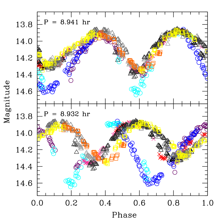
Figure 4: 1999 data phased to the 8.941 hour period (top panel) and the 8.932 hr (bottom panel). The magnitudes are m_R^∗ (given in column (4) of Table LABEL:t:photometry). The midpoint of each image was used and then corrected for the light travel time, with zero phase set at perihelion (1999 September 8.424). The points are as given in Figure 1.

We applied this technique to the m_R^∗ data given in column (4) of Table LABEL:t:photometry, finding an observed, i.e. synodic, period of 8.941 $\pm$ 0.002 hr for the combined dataset (April–June). We examined all period solutions between 4.47 hr (the single-peaked solution) and 13.41 hr (the triple-peaked solution) and 8.941 hr (the double-peaked solution) is the only viable solution between these extremes. The double-peaked shape is expected for a triaxial ellipsoid and was observed by previous authors in 1988 and 1994. We plot the m_R^∗ data phased to 8.941 hr in the top panel of Figure 4. The bottom panel is phased to 8.932 hr (the period solution from 1988, discussed in the following subsection).

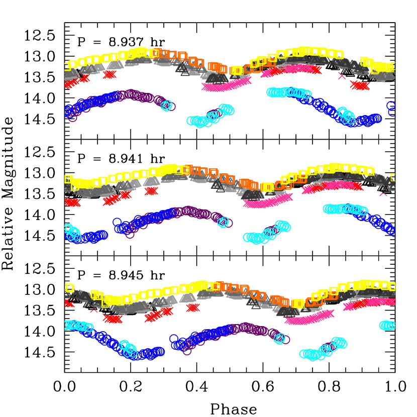
Figure 5: Our 1999 data phased to 8.937 hr (top panel), 8.941 hr (middle panel), and 8.945 hr (bottom panel). The magnitudes are m_R^∗ (given in column (4) of Table LABEL:t:photometry) offset by $-$0.015 magnitudes per day from 1999 April 17. This offset has been applied for display purposes to minimize overlapping data so the trend in the phasing of extrema is more apparent. The midpoint of each image was used and then corrected for the light travel time before phasing, with zero phase set at perihelion (1999 September 8.424). The symbols are as given in Figure 1. By phasing the data in this manner, we found a best period of 8.941 hr and an uncertainty of $\pm$0.002 hr.

The uncertainty in the period was estimated from the smallest offset that produced lightcurves that were visibly out of phase. Figure 5 illustrates an exaggeration of this process using three periods: 8.937 hr (top), 8.941 (middle) and 8.945 (bottom). Note that these periods are separated by double the estimated error to emphasize the trend in the location of the extrema. We plot the m_R^∗ data offset vertically by $-$0.015 mag day^-1 since 1999 April 17 to better show the chronological progression of the lightcurves. In the top panel, later lightcurves (higher on the plot) occur at a later phase, while in the bottom panel later lightcurves occur at an early phase. This clearly illustrates that the correct solution is between the two, making it easy to identify 8.941 hr as the optimal period. The inclusion of the April data is vital for this process, as the larger separation between April and the later datasets decreases the range of possible solutions.

For comparison, we also conducted period searches using Fourier (Deeming, 1975) and phase dispersion minimization (PDM; Stellingwerf (1978)) techniques. The Fourier routine “Period04” (Lenz & Breger, 2005) found a single-peaked period of 4.4705 $\pm$ 0.0001 hr. Since we expect the lightcurve to be double-peaked, this implies a rotation period twice as long, or 8.9409 $\pm$ 0.0002 hr (the difference in the last digit is due to rounding). The routine determined an uncertainty in frequency and we converted this to a period uncertainty, although we note that the uncertainty of 0.0002 hr seems unrealistically small. We used our own PDM routine, which found a double-peaked period of 8.941 $\pm$ 0.005 hr. We estimated the period uncertainty by finding the range of solutions that had $\theta$ (a measure of the goodness of fit) within 50% of the minimum $\theta$. The agreement between methods confirms the robustness of our period solution.

3.2 Different Rotation Periods Due to Geometry?

The default rotation period obtained by simply phasing the data is the synodic period, the length of time until the brightness appears the same from the Earth. This period changes during the apparition because the illuminated portion of the nucleus seen by the Earth varies as both the Earth and the comet move in their orbits. The sidereal rotation period is the rotation period relative to a fixed position in inertial space. A third period is the solar period, which is the time until the Sun is in the same place in the sky as seen by the comet. Because the synodic and solar rotation periods depend on the orientation of the rotational pole, converting them to a sidereal period requires a pole solution.

Since the synodic period also depends on the position of the Earth, we must consider the geometry of the Earth-comet-Sun system during our observations to confirm that the synodic period changes slowly enough that measuring a single synodic period for the whole 10-week time span is sensible. As seen from the comet, the ecliptic longitude of the Earth (column (9) of Table 1) and the ecliptic latitudes of the Sun and Earth all changed by less than 5^∘ during our observations, resulting in minimal changes to the measured rotation period. While the ecliptic longitude of the Sun as seen from the comet (column (10) of Table 1) changed by $\sim$30^∘, the net effect on the rotation period was still small due to the likely pole orientation (see discussion below), and obtaining a single (synodic) rotation period for the whole time span was valid.

To confirm this, we investigated the synodic rotation periods which would be observed at different times for pole solutions within 20^∘ in the comet’s orbital coordinate system (obliquity and azimuthal angle) of the pole solution given by Sekanina (1987). This range of solutions was chosen to include the pole solution found by Sekanina (1991) for the 1988 apparition and a preliminary pole solution for our 1999 coma morphology data (we will explore this in detail in Paper 2). We considered three runs discretely: April 17–19, May 26–27, and June 22–23 (the June 8–11 run gave similar results to the June 22–23 run), and determined the synodic–sidereal offset which would be observed for all pole solutions under consideration. The difference between the synodic and sidereal periods was 0.000 to $+$0.003 hr during the April run, 0.000 to $+$0.002 hr during the May run, and $-$0.001 to $+$0.001 hr during the late-June run. Considering the entire 10-week interval as a single large run (i.e. April 17–June 23), the best synodic period differed from the sidereal period by 0.000 to $+$0.002 hr. Thus, the changing geometry during our observations did not introduce an error in the period determined from the entire run larger than the estimated uncertainty in the synodic period of 0.002 hr (although if the April run was considered by itself, the maximum difference was 0.003 hr). Note that the sign of the synodic–sidereal difference reverses for a pole orientation in the opposite direction, i.e. when the comet has retrograde spin and “north” is defined in the opposite hemisphere.

The above example suggests that changes in the synodic period may be detectable during an apparition. We considered subsets of our 1999 data to look for such a change. There was no discernible difference when the rotation period was determined using all the April and May data or all the May and June data (both intervals gave acceptable solutions from 8.940–8.942 hr with a best period of 8.941 hr). We also determined the synodic period between every combination of individual nights from different runs for which a synodic period could be determined. We phased each pair of nights and defined the midpoint between the two nights as the date corresponding to the measured synodic period. This method suggests an increase in the synodic period of $\sim$0.002 hr from early-May to mid-June, although the scatter in the individual synodic measurements is very large and the range of acceptable solutions for each pair is generally at least $\pm$ 0.002 hr. If correct, this requires that the “north” pole be in the opposite hemisphere as was determined by Sekanina (1987), i.e. retrograde rather than prograde rotation.

3.3 Reanalysis of the 1988 Data

We reanalyzed the publicly available datasets from 1988 (Jewitt & Luu (1989), A’Hearn et al. (1989), and Wisniewski (1990)), defining zero phase at perihelion (1988 September 16.738). The observing scenarios for these datasets are summarized in Table LABEL:t:obs_summary_1988. Jewitt & Luu (1989) removed coma from their June data but not the February or April data. A’Hearn et al. (1989) obtained optical and thermal IR data simultaneously on different telescopes, and removed coma from the optical data but not from the thermal IR data, which were shown to be nearly free of coma. Wisniewski (1990) did not remove coma from his data. The 1987 data from Jewitt & Meech (1988) were not included in the 1988 period determination because they were too far away in time and were at a much different location in the orbit, making it impossible to directly compare the synodic rotation periods.

We normalized the published magnitudes to m_R(1,1,0) using $\beta$ = 0.032 mag deg^-1 as was used with our 1999 data. After this normalization, the optical magnitudes still differed by several tenths of a magnitude between runs and authors. We therefore adjusted all the lightcurves to peak at the same magnitude for the maximum near zero phase by applying nightly $\Delta$m₂ values (given in column (12) of Table LABEL:t:obs_summary_1988). We call these data m_R^∗, and used them for our period search. $\Delta$m₂ corrects for nightly differences between datasets due to differences in the extinction correction, absolute calibration, and coma removal (or lack thereof). We do not list a $\Delta$m₂ for the A’Hearn et al. (1989) 4845 Å data, as we did not use them when phasing the data since the 4845 Å and 6840 Å data were obtained alternately throughout both nights, and their lightcurve shapes were nearly identical (although the 6840 Å data were brighter).

Visually scanning the 1988 data for a double-peaked solution, as was done for our 1999 data, yielded a period of 8.932 $\pm$ 0.001 hr. This period agrees with the synodic periods determined for the 1988 data by Sekanina (1991) (8.931 $\pm$ 0.001 hr, given in his Table 5) and Mueller & Ferrin (1996) (8.933 $\pm$ 0.002).

The viewing geometry in 1988 was nearly identical to the viewing geometry in 1999; the ecliptic latitudes of the Earth and Sun changed minimally and the ecliptic longitudes of the Earth and Sun (given in columns (9) and (10), respectively, in Table LABEL:t:obs_summary_1988) mimicked the changes in 1999. As with the 1999 data (Section 3.1), we considered discrete runs spanning the range of 1988 observations: February 24–28, April 8–12, May 18–22, and June 19–23, and determined the synodic–sidereal difference during each run for the range of pole solutions. Because of the similar viewing geometry, the synodic–sidereal difference was almost the same as in 1999: $+$0.001 to $+$0.002 hr for February 24–28, $+$0.001 to $+$0.002 hr for April 8–12, 0.000 to $+$0.001 hr for May 18–22, and $-$0.001 to $+$0.001 hr for June 19–23. Considering the entire 1988 time span from February 25 until June 30 as a single large run, the difference in the synodic and sidereal rotation periods was 0.000 to $+$0.002 hr for the range of pole solutions. As with 1999, the synodic–sidereal difference changes sign for a pole orientation in the opposite direction.

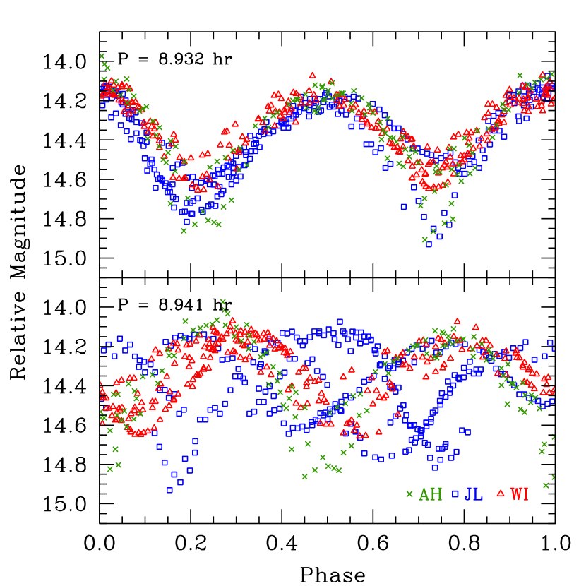
Figure 6: 1988 data from the literature phased to the 8.932 hour period (top panel) and the 8.941 hr (bottom panel). The published data have been normalized to m_R(1,1,0) and offset by $\Delta$m₂ (given in Table LABEL:t:obs_summary_1988) to peak at the same magnitude. The times are as given in the literature and corrected for the light travel time, and zero phase was defined at perihelion (1988 September 16.738). The green crosses (AH) are A’Hearn et al. (1989), the blue squares (JL) are Jewitt & Luu (1989), and the red triangles (WI) are Wisniewski (1990).

Thus we can directly compare our 1988 solution (8.932 hr) with our 1999 solution (8.941 hr). In Figure 6 we plot the 1988 m_R^∗ data phased to our period solution from 1988 in the top panel and to our period solution from 1999 in the bottom panel. Similarly, we plot our 1999 m_R^∗ data phased to 8.941 hr (top panel) and 8.932 hr (bottom panel) in Figure 4. Figures 4 and 6 demonstrate that the rotation periods were clearly different in 1988 and 1999. Since the synodic periods differed by $\sim$0.009 hr and synodic–sidereal offsets were similar each apparition, we can conclude that the sidereal periods also differed by $\sim$0.009 hr, and thus the rotation period increased from 1988 to 1999.

We looked for a change in the synodic period during the 1988 observations by phasing every combination of pairs of observing runs, e.g. Jewitt & Luu (1989)’s February data with A’Hearn et al. (1989)’s June data, Jewitt & Luu (1989)’s February data with Wisniewski (1990)’s June data, etc. Assigning the date of each pair as the midpoint between the two runs, there was no discernible trend in the measured synodic period over time, with acceptable values varying from 8.931–8.933 hr with a typical uncertainty of $\pm$0.001 hr. This is consistent with the conclusions of Jewitt & Luu (1989) who found no change in the rotation period within their uncertainty when analyzing their February, April, and June data as discrete sets. In contrast, Sekanina (1991) found a decrease in the synodic period during the 1988 observations of $\sim$0.003 hr (his Table 5 and Figure 7). These discrepancies and our possible finding of a slight increase in the rotation period in 1999 (Section 3.1) suggest that Sekanina (1987)’s pole solution may not be definitive, with the alternate sense of rotation possible as well (resulting in a “north” pole in the exact opposite position). We will use the coma morphology visible in our post-perihelion 1999 images, combined with data we will obtain in 2010, to attempt to determine a more robust pole solution in Paper 2.

3.4 Reanalysis of the 1994 Data

We also reanalyzed the Mueller & Ferrin (1996) data from 1994, normalizing the published magnitudes to m_R(1,1,0) and visually scanning for possible solutions. The data do not yield an unambiguous double-peaked lightcurve due to undersampling. Mueller & Ferrin (1996) found five possible solutions: 8.877 hr, 8.908 hr, 8.939 hr, 8.971 hr, and 9.002 hr, and we concur with their results. Only one of these, 8.939 hr, is within the uncertainty of our 1999 solution (8.941 $\pm$ 0.002 hr).

Using the same range of pole solutions as in Section 3.2, we find the maximum difference between the synodic and sidereal periods in October–December 1994 was smaller than $-$0.001 hr (actually about $-$1 s), in agreement with the difference found by Mueller & Ferrin (1996). Thus, the expected difference between the synodic and sidereal rotation periods is much less than the difference between the five possible solutions. Furthermore, since there were no intervening perihelion passages between the 1994 and 1999 observations, the sidereal rotation period was likely unchanged between these observations. Therefore, we rule out the remaining four possible solutions from Mueller & Ferrin (1996), and conclude that Tempel 2 had spun-down by $\sim$0.009 hr ($\sim$ 32 s) between the 1988 and 1994 determinations, which spanned two perihelion passages, and was unchanged between the 1994 post-perihelion observations and our 1999 pre-perihelion observations.

3.5 Coma Contamination and Lightcurve Amplitude

Tempel 2 was non-stellar in appearance throughout our 1999 observations. The presence of a coma suppressed the amplitude of the lightcurve, with the suppression increasing later in the apparition as activity increased. The mean coma removed from the 6 arcsec radius monitoring aperture was 0.20 mag from April 17–19, 0.27 mag from May 26–27, 0.40 mag from June 8–11, and 0.65 mag from June 22–23. We measured lightcurve amplitudes ranging from 0.2–0.5 mag prior to removal of the coma. After coma removal, the April 17–19 data exhibited amplitudes of $\sim$0.75 mag while all subsequent runs had amplitudes of 0.45–0.50 mag. If a quadratic fit to the coma was used instead of a linear fit, the amplitudes increased to $\sim$0.80 in April and 0.50–0.60 in May and June. However, note that as discussed in Section 2.4, we opted for a more conservative linear fit rather than a higher order fit because the higher order fits varied more from image to image and produced less reliable results. Our measured amplitudes in 1999 are similar to the maximum optical amplitudes reported by other authors in 1988 when the comet was at a similar viewing geometry and activity level: 0.65 $\pm$ 0.05 mag in February and 0.60 $\pm$ 0.05 mag in April (no coma removal; Jewitt & Luu (1989)), 0.5 mag in May (no coma removal; Wisniewski (1990)), and 0.7 $\pm$ 0.1 mag in June (coma removed; Jewitt & Luu (1989)).

A’Hearn et al. (1989) measured an amplitude of 0.8 mag in their 10.1 $\mu$m data in 1988 June, exceeding all measured optical amplitudes at similar times in both 1988 and 1999. While the amplitudes measured by ourselves and others approach the thermal IR amplitude, all are somewhat lower, and even a quadratic coma removal from our data cannot bring the amplitudes into agreement. This discrepancy raises two possible interpretations. First, the coma removal techniques employed here and by Jewitt & Luu (1989) and A’Hearn et al. (1989) are not adequately estimating the coma inside the photometric aperture. To push the amplitude up to $\sim$0.80, 50–150% more coma would need to be removed from our May and June data, requiring a significantly steeper curve than even a quadratic fit. Alternatively, the convergence of multiple authors on an optical amplitude of 0.6–0.7 mag in 1988 June and 1999 June may indicate that this is in fact the correct optical amplitude, and is different from the thermal IR amplitude. This possibility was suggested by A’Hearn et al. (1989) based on work by Brown (1985) who showed that the amplitude of the thermal IR lightcurve may be dependent on both wavelength and elongation.

The varying lightcurve amplitudes will be utilized in Paper 2 when we determine the pole solution using the coma morphology from 1999 and 2010. As the viewing geometry varies during an apparition, the amplitude of the lightcurve will vary because different cross sections of the nucleus are observed. Thus, the lightcurve amplitudes will be useful in refining the pole solution and will help in constraining the shape of the nucleus.

We looked for evidence of periodicity in the coma signal by plotting both the total flux and flux per square arcsec in each photometric annulus as a function of rotational phase. What structure is visible on individual nights does not repeat in a coherent manner from night to night or from run to run. There was also no evidence of propagation of any features (either a maximum or minimum signal) outwards during a night. This is consistent with the analyses of Jewitt & Luu (1989) and A’Hearn et al. (1989) who did not see a rotation signal in their data.

3.6 Lightcurve Asymmetry

The rotational lightcurve in 1999 is somewhat asymmetric, allowing identification of certain features many rotations apart and eliminating $N-0.5$, $N+0.5$, $N+1.5$… (where $N$ is the number of cycles) as possible solutions. This conclusively rules out the single- and triple-peaked solutions and reduces the uncertainty in the period determination since it halves the number of possible rotations. Any clear description of the lightcurve shape is made challenging because it is never observed completely on a given night. However, we note the following apparently repeated features: The minimum near 0.6 phase is deeper and steeper than the minimum near 0.1 phase when comparing lightcurves from the same observing run. There is a shoulder in the rising portion between 0.15 and 0.30 phase. Finally, while there are no nights in which both maxima were clearly observed, the maximum near 0.85 phase may be slightly higher than the maximum near 0.35 phase. We see evidence for each of these features in the 1988 data when discrete observing runs are considered. The features are also seen in the 1994 data from Mueller & Ferrin (1996), although since the viewing geometry was very different, we cannot be sure that they correspond to the same topographic features on the nucleus.

4 Summary and Discussion

We imaged Tempel 2 on 32 nights from 1999 April until 2000 March. We present here R-band nucleus lightcurves obtained on 11 of these nights from April through June (prior to perihelion), a total of 892 data points. Absolute calibrations and nightly extinction corrections were determined on photometric nights, and were applied to non-photometric nights to extract usable lightcurves. Field stars in the image were monitored on all nights and were used as comparison stars to correct the comet magnitude on non-photometric nights. A median coma was determined each night and removed from all images on the night. All magnitudes were normalized to $r$ = $\Delta$ = 1 AU and $\alpha$ = 0^∘. A final adjustment, which accounts for uncertainties in the calibrations that tend to create nightly magnitude offsets such as the application of absolute calibrations on non-photometric nights, was applied to make each night peak at the same magnitude.

We determined a synodic rotation period of 8.941 $\pm$ 0.002 hr; no other double-peaked solutions exist. Our dataset is sufficient to rule out all aliases other than the single- and triple-peaked solutions, and these are ruled out by the differences in shape and brightness between the two minima. Our period matches one of the possible periods obtained by Mueller & Ferrin (1996) from post-perihelion data in 1994 (during the same inter-perihelion time as our 1999 data) and rules out their other four possible solutions. We reanalyzed published data from 1988 using the same analysis techniques and found a synodic rotation period of 8.932 $\pm$ 0.001 hr. Our 1999 data cannot be fit by the rotation period from 1988, nor can the 1988 data be fit by the rotation period from 1999, even though the comet had nearly identical viewing geometries during the two sets of observations. Thus, we conclude that Tempel 2 spun-down by 0.009 hr ($\sim$32 s) from 1988 to 1999, an interval that included two perihelion passages.

This marks the first conclusive measurement of spin-down in a comet, although three comets have shown possible evidence of spin-up: 9P/Tempel 1 (Belton & Drahus, 2007; Chesley et al., 2010), 2P/Encke (Fernández et al., 2005), and Comet Levy (1990c) (Schleicher et al., 1991; Feldman et al., 1992). Modeling by Samarasinha & Belton (1995), Neishtadt et al. (2002), Gutiérrez et al. (2003), and others has shown that either spin-up or spin-down is possible, with spin-up more likely in the long run. These simulations have shown that under certain conditions the spin period can change by much larger amounts in a single orbit (e.g. typical changes of 0.01–10 hr per orbit according to Gutiérrez et al. (2003)) than the measured change of 0.009 hr in two orbits for Tempel 2. Thus, the measured spin-down of 10P/Tempel 2 is probably not exceptional, and comparable changes in period could likely be measured in other comets if similarly high quality data were obtained over several epochs.

Possible causes of a change in spin-state are summarized by Samarasinha et al. (2004). The spin-down of Tempel 2 may have been caused by either a one-time event or by recurring torquing each orbit. Scenarios for causing a one-time change in rotation period include a short-lived, freshly exposed active region (causing temporary torquing), fragmentation (changing the moment of inertia), collision with another object, and tidal torquing from Jupiter. The orbit of Tempel 2 is well known and tidal torquing from Jupiter should not have been significant or more severe between 1988 and 1999 than on other recent orbits. Collisions are rare in the current solar system, and any collision significant enough to alter the rotation period of Tempel 2 would likely have resulted in an increase in brightness upon subsequent orbits, which has not been seen. Fragmentation is known to be relatively common, occurring on average at least once per century per comet (c.f. Chen & Jewitt (1994); Weissman (1980)). However, there is no evidence for Tempel 2 having split, such as a companion nucleus or a sustained increase in brightness as was observed in 73P/Schwassmann-Wachmann 3 (Ferrín, 2010). A new active region could be created by fragmention, impact, or outburst. Since outbursts are known to occur far more frequently than fragmentation or impacts, an outburst is the most plausible explanation for a one-time change in the rotation period. If the change in the period was caused by a unique event such as an outburst, it could have occurred anywhere in the orbit and we would expect no change in the rotation period on subsequent orbits.

It is challenging to devise a mechanism that is strong enough to affect the rotation period but lasts for a short time (less than one orbit). Thus, we suspect the spin-down is due to torques on the nucleus caused by asymmetric outgassing. This is believed to be the most common means of changing the spin state of a comet (c.f. Samarasinha et al. (2004)). Seasonal illumination of an active region could cause torquing which slows the rotation of the nucleus by a comparable amount each orbit. In the case of Tempel 2, the torquing likely occurs near or shortly after perihelion, when the comet is most active, although the length of time over which the torquing may occur is unknown. Since Tempel 2 reached perihelion twice between the 1988 and 1999 observations, in this, our preferred scenario, the rotation period must be changing by $\sim$16 s each orbit.

Tempel 2 reached perihelion on 2010 July 4, and we encourage its observation throughout the apparition to determine the rotation period. Due to a perturbation by Jupiter between the 1999 and 2005 apparitions, the viewing geometry is different in 2010 than in 1988 or 1999. The post-perihelion viewing geometry will be better this apparition and the comet will be visible longer each night. The smaller post-perihelion $\Delta$ in 2010 will provide better spatial resolution, making it easier to separate the nucleus and coma signals even though the coma is more extensive after perihelion. This may allow measurement of a nucleus lightcurve after perihelion, despite increased coma contamination relative to the pre-perihelion measurements in 1988, 1994, and 1999.

Assuming the spin-down is recurrent each orbit, we predict that the pre-perihelion rotation period should be $\sim$32 s longer than in 1999 as there have been two intervening perihelion passages (1999 September 8 and 2005 February 15) since our data were obtained in 1999. If the pole position given by Sekanina (1987) is correct, the sidereal rotation period should be 8.950 $\pm$ 0.003 hr. Since it is unknown if the spin-down is caused by an instantaneous impulsive event or a steady change over an extended period of time, we cannot estimate the rotation period that might be observed shortly after perihelion in 2010. Observations long enough after perihelion to allow the torquing to have taken effect should reveal an additional lengthening of the sidereal rotation period by $\sim$16 s relative to the pre-perihelion 2010 period. Using again the pole solution of Sekanina (1987), this would yield a sidereal period 8.954 $\pm$ 0.004 hr.

We have begun to observe Tempel 2 in 2010 and will combine these new data with our observations obtained during its active phase in 1999 as a follow up to the current paper. As of August 2010 (when the revised manuscript was submitted), we are unaware of any period determinations from 2010 observations. In Paper 2 we will use the different viewing geometry provided by the 2010 apparition to investigate the pole orientation and the location and activity of any jets. We hope to determine the rotation period in 2010, and possibly obtain additional post-perihelion observations after activity has subsided in 2011 or later to resolve whether the comet spins down each orbit. With its relatively low inclination ($i$ $\sim$ 12^∘) and perihelion close to the Earth’s orbit ($q$ $\sim$ 1.4 AU), Tempel 2 is frequently on the short list of targets for comet missions, making further study highly desirable.

Table 1: Summary of Tempel 2 observations and geometric parameters in 1999. 

UT	UT	Tel.	CCD	$r$	$\Delta$	$\alpha$	$\Delta$t	Ecl. Long.	Ecl. Long.	$\Delta$m1	$\Delta$m2	$\sigma$${}_{m_{R}}$	Conditions
Date	Range	Diam.		(AU)	(AU)	(∘)	(hr)	Earth (∘)	Sun (∘)
Apr 17	7:48–11:55	1.8-m	SITe	2.025	1.275	24.0	0.177	80.1	56.3	$-$2.84	$-$0.02	0.02–0.04	thin clouds
Apr 18	7:20–12:11	1.8-m	SITe	2.020	1.262	23.8	0.176	80.3	56.7	$-$2.81	+0.08	0.02–0.06	thin clouds
Apr 19	6:53–12:10	1.8-m	SITe	2.014	1.248	23.7	0.174	80.5	57.1	$-$2.77	$+$0.03	0.03	photometric
May 26	6:37–11:22	1.8-m	SITe	1.807	0.839	13.9	0.117	81.9	72.2	$-$1.36	+0.15	0.01	thin clouds
May 27	7:43–11:30	1.8-m	SITe	1.802	0.831	13.6	0.116	81.8	72.7	$-$1.33	+0.26	0.01	thin clouds
Jun 08	7:05–11:14	1.1-m	TI	1.741	0.748	10.7	0.104	80.1	78.4	$-$0.92	…	0.02	photometric
Jun 09	4:45–09:36	1.1-m	TI	1.736	0.743	10.6	0.103	80.0	78.8	$-$0.90	…	0.03	photometric
Jun 10	4:34–11:17	1.1-m	TI	1.731	0.737	10.5	0.102	79.7	79.3	$-$0.87	$-$0.02	0.02	photometric
Jun 11	4:30–09:35	1.1-m	TI	1.726	0.732	10.4	0.102	79.6	79.8	$-$0.85	…	0.02	photometric
Jun 22	7:29–11:08	1.1-m	TI	1.675	0.685	12.4	0.095	77.5	85.4	$-$0.69	$-$0.07	0.02–0.06	thin clouds
Jun 23	3:57–11:04	1.1-m	TI	1.671	0.682	12.7	0.095	77.4	85.9	$-$0.69	$-$0.07	0.02–0.04	photometric

Table 2: Table of photometry

UT Date	UT	mR	mR*
Apr 17	07.848	16.93	14.38
Apr 17	07.915	16.90	14.34
Apr 17	07.952	17.00	14.47
Apr 17	07.989	16.90	14.34
Apr 17	08.038	16.83	14.25
Apr 17	08.076	16.89	14.33
Apr 17	08.112	16.84	14.26
Apr 17	08.201	16.76	14.16
Apr 17	08.294	16.83	14.24
Apr 17	08.331	16.74	14.13
Apr 17	08.368	16.73	14.13
Apr 17	08.421	16.73	14.13
Apr 17	08.458	16.68	14.06
Apr 17	08.495	16.69	14.07
Apr 17	08.547	16.72	14.11
Apr 17	08.637	16.71	14.10
Apr 17	08.674	16.68	14.07
Apr 17	08.711	16.73	14.12
Apr 17	08.748	16.71	14.10
Apr 17	08.785	16.67	14.04
Apr 17	08.821	16.63	14.00
Apr 17	08.893	16.64	14.02
Apr 17	08.972	16.65	14.02
Apr 17	09.067	16.62	13.99
Apr 17	09.104	16.59	13.94
Apr 17	09.142	16.60	13.96
Apr 17	09.179	16.58	13.93
Apr 17	09.216	16.61	13.98
Apr 17	09.253	16.58	13.93
Apr 17	09.315	16.58	13.93
Apr 17	09.421	16.56	13.91
Apr 17	09.486	16.55	13.91
Apr 17	09.523	16.54	13.90
Apr 17	09.560	16.56	13.92
Apr 17	09.597	16.56	13.91
Apr 17	09.634	16.59	13.96
Apr 17	09.671	16.57	13.93
Apr 17	09.716	16.60	13.96
Apr 17	09.807	16.60	13.97
Apr 17	09.844	16.63	14.00
Apr 17	09.881	16.62	13.98
Apr 17	09.918	16.62	13.99
Apr 17	09.955	16.62	13.99
Apr 17	09.992	16.62	13.99
Apr 17	10.037	16.64	14.01
Apr 17	10.219	16.67	14.05
Apr 17	10.288	16.70	14.09
Apr 17	10.325	16.68	14.07
Apr 17	10.362	16.71	14.11
Apr 17	10.399	16.73	14.13
Apr 17	10.436	16.75	14.14
Apr 17	10.473	16.75	14.16
Apr 17	10.604	16.79	14.21
Apr 17	11.689	16.95	14.41
Apr 17	11.726	16.95	14.41
Apr 17	11.763	16.93	14.38
Apr 17	11.800	16.94	14.39
Apr 17	11.890	16.91	14.35
Apr 18	07.681	16.47	13.89
Apr 18	07.718	16.44	13.86
Apr 18	07.755	16.46	13.89
Apr 18	07.792	16.48	13.91
Apr 18	07.829	16.48	13.90
Apr 18	07.867	16.47	13.90
Apr 18	07.906	16.49	13.91
Apr 18	07.943	16.51	13.94
Apr 18	07.980	16.55	13.99
Apr 18	08.017	16.55	13.99
Apr 18	08.054	16.61	14.05
Apr 18	08.091	16.62	14.06
Apr 18	08.160	16.61	14.05
Apr 18	08.234	16.63	14.08
Apr 18	08.395	16.68	14.14
Apr 18	08.432	16.69	14.15
Apr 18	08.469	16.74	14.21
Apr 18	08.506	16.66	14.12
Apr 18	08.543	16.78	14.25
Apr 18	08.580	16.73	14.20
Apr 18	08.621	16.74	14.21
Apr 18	08.702	16.83	14.31
Apr 18	08.739	16.81	14.29
Apr 18	08.777	16.84	14.33
Apr 18	08.814	16.83	14.32
Apr 18	08.851	16.89	14.39
Apr 18	08.888	16.90	14.40
Apr 18	08.962	16.93	14.44
Apr 18	09.028	16.98	14.50
Apr 18	09.109	17.00	14.53
Apr 18	09.146	16.99	14.52
Apr 18	09.183	17.04	14.57
Apr 18	09.220	17.01	14.54
Apr 18	09.258	17.03	14.56
Apr 18	09.295	17.05	14.59
Apr 18	09.332	17.07	14.61
Apr 18	09.429	17.07	14.61
Apr 18	09.535	17.06	14.60
Apr 18	09.611	17.02	14.55
Apr 18	09.649	17.03	14.56
Apr 18	09.686	17.01	14.54
Apr 18	09.723	17.01	14.53
Apr 18	09.760	17.04	14.57
Apr 18	09.797	17.07	14.61
Apr 18	09.836	17.04	14.58
Apr 18	09.873	17.01	14.54
Apr 18	09.910	17.01	14.54
Apr 18	09.947	16.98	14.51
Apr 18	09.985	16.98	14.50
Apr 18	10.022	16.98	14.50
Apr 18	10.062	16.99	14.51
Apr 18	10.391	16.73	14.20
Apr 18	10.460	16.86	14.35
Apr 18	10.541	16.87	14.37
Apr 18	10.579	16.85	14.35
Apr 18	10.616	16.83	14.32
Apr 18	10.653	16.80	14.28
Apr 18	10.690	16.90	14.40
Apr 18	10.811	16.80	14.29
Apr 18	10.917	16.75	14.22
Apr 18	10.959	16.77	14.24
Apr 18	10.996	16.67	14.13
Apr 18	11.033	16.74	14.22
Apr 18	11.070	16.74	14.21
Apr 18	11.107	16.71	14.18
Apr 18	11.144	16.70	14.16
Apr 18	11.210	16.68	14.14
Apr 18	11.277	16.67	14.13
Apr 18	11.356	16.62	14.07
Apr 18	11.393	16.64	14.09
Apr 18	11.431	16.64	14.09
Apr 18	11.468	16.66	14.12
Apr 18	11.505	16.61	14.06
Apr 18	11.542	16.61	14.06
Apr 18	11.623	16.60	14.05
Apr 18	11.664	16.57	14.01
Apr 18	11.702	16.57	14.01
Apr 18	11.739	16.58	14.02
Apr 18	11.776	16.56	14.01
Apr 18	11.813	16.55	13.99
Apr 18	11.851	16.54	13.98
Apr 18	11.902	16.53	13.96
Apr 19	07.129	16.77	14.22
Apr 19	07.170	16.80	14.25
Apr 19	07.208	16.74	14.18
Apr 19	07.824	17.07	14.57
Apr 19	07.889	17.06	14.57
Apr 19	07.956	17.08	14.59
Apr 19	07.993	17.06	14.56
Apr 19	08.031	17.09	14.61
Apr 19	08.068	17.12	14.64
Apr 19	08.105	17.07	14.58
Apr 19	08.142	17.10	14.62
Apr 19	08.185	17.07	14.59
Apr 19	08.281	17.10	14.62
Apr 19	08.319	17.02	14.52
Apr 19	08.356	16.99	14.48
Apr 19	08.393	17.02	14.52
Apr 19	08.430	16.96	14.45
Apr 19	08.467	17.03	14.53
Apr 19	08.606	16.93	14.41
Apr 19	08.692	16.82	14.27
Apr 19	08.730	16.87	14.34
Apr 19	08.766	16.82	14.28
Apr 19	08.804	16.86	14.33
Apr 19	08.841	16.83	14.29
Apr 19	08.878	16.87	14.34
Apr 19	09.987	16.49	13.89
Apr 19	10.024	16.50	13.91
Apr 19	10.062	16.48	13.88
Apr 19	10.099	16.50	13.90
Apr 19	10.136	16.49	13.90
Apr 19	10.172	16.49	13.90
Apr 19	10.211	16.49	13.90
Apr 19	10.292	16.51	13.91
Apr 19	10.329	16.48	13.89
Apr 19	10.366	16.48	13.88
Apr 19	10.384	16.48	13.88
Apr 19	10.441	16.48	13.88
Apr 19	10.478	16.49	13.89
Apr 19	10.578	16.48	13.88
Apr 19	10.658	16.49	13.90
Apr 19	10.696	16.50	13.91
Apr 19	10.732	16.51	13.92
Apr 19	10.769	16.51	13.92
Apr 19	10.806	16.50	13.91
Apr 19	10.844	16.51	13.92
Apr 19	10.907	16.53	13.94
Apr 19	10.974	16.53	13.95
Apr 19	11.889	16.89	14.36
Apr 19	11.926	16.87	14.35
Apr 19	11.964	16.91	14.39
Apr 19	12.001	17.01	14.54
Apr 19	12.038	16.92	14.44
Apr 19	12.076	16.92	14.44
Apr 19	12.113	16.95	14.47
Apr 19	12.151	17.01	14.55
May 26	06.640	14.91	13.99
May 26	06.679	14.89	13.97
May 26	06.716	14.88	13.95
May 26	06.760	14.87	13.95
May 26	06.801	14.88	13.95
May 26	06.838	14.86	13.93
May 26	06.875	14.85	13.92
May 26	06.912	14.85	13.92
May 26	06.992	14.84	13.91
May 26	07.029	14.84	13.91
May 26	07.066	14.84	13.90
May 26	07.103	14.82	13.89
May 26	07.140	14.83	13.90
May 26	07.191	14.84	13.91
May 26	07.227	14.83	13.90
May 26	07.264	14.84	13.90
May 26	07.302	14.83	13.89
May 26	07.339	14.81	13.87
May 26	07.517	14.82	13.88
May 26	07.554	14.82	13.88
May 26	07.591	14.81	13.88
May 26	07.631	14.82	13.88
May 26	07.668	14.82	13.88
May 26	07.705	14.82	13.89
May 26	07.742	14.82	13.88
May 26	07.779	14.84	13.90
May 26	07.819	14.83	13.89
May 26	07.857	14.84	13.91
May 26	07.894	14.85	13.92
May 26	07.931	14.85	13.91
May 26	07.968	14.85	13.93
May 26	08.935	15.10	14.25
May 26	08.974	15.13	14.30
May 26	09.011	15.12	14.28
May 26	09.048	15.12	14.29
May 26	09.085	15.14	14.31
May 26	09.122	15.13	14.30
May 26	09.163	15.13	14.30
May 26	09.200	15.14	14.31
May 26	09.237	15.14	14.31
May 26	09.274	15.13	14.30
May 26	10.044	15.12	14.29
May 26	10.081	15.11	14.27
May 26	10.119	15.11	14.26
May 26	10.156	15.10	14.26
May 26	10.195	15.08	14.23
May 26	10.232	15.07	14.21
May 26	10.269	15.05	14.18
May 26	10.307	15.04	14.18
May 26	10.344	15.03	14.17
May 26	10.484	15.01	14.13
May 26	10.521	14.99	14.11
May 26	10.558	15.00	14.11
May 26	10.596	15.00	14.11
May 26	10.632	14.98	14.10
May 26	11.187	14.94	14.04
May 26	11.225	14.94	14.04
May 26	11.262	14.92	14.01
May 26	11.299	14.92	14.02
May 26	11.353	14.92	14.02
May 27	07.732	15.12	14.33
May 27	07.777	15.12	14.33
May 27	07.820	15.13	14.34
May 27	07.859	15.15	14.36
May 27	07.899	15.14	14.36
May 27	07.936	15.14	14.35
May 27	07.974	15.15	14.36
May 27	08.012	15.15	14.36
May 27	08.050	15.14	14.36
May 27	08.088	15.15	14.36
May 27	08.129	15.15	14.37
May 27	08.168	15.14	14.35
May 27	08.206	15.13	14.34
May 27	08.243	15.13	14.34
May 27	08.280	15.13	14.34
May 27	08.317	15.12	14.32
May 27	08.356	15.12	14.32
May 27	08.394	15.10	14.30
May 27	08.431	15.10	14.30
May 27	08.468	15.10	14.30
May 27	08.505	15.08	14.28
May 27	08.544	15.07	14.27
May 27	08.581	15.06	14.25
May 27	08.618	15.04	14.23
May 27	08.655	15.03	14.22
May 27	08.692	15.03	14.21
May 27	08.734	15.02	14.20
May 27	08.771	15.01	14.19
May 27	08.808	15.01	14.18
May 27	08.846	15.00	14.18
May 27	08.883	15.00	14.18
May 27	09.303	14.87	14.02
May 27	09.340	14.88	14.03
May 27	09.377	14.87	14.02
May 27	09.414	14.87	14.02
May 27	09.451	14.86	14.00
May 27	09.915	14.78	13.91
May 27	09.952	14.78	13.91
May 27	09.989	14.77	13.90
May 27	10.026	14.77	13.90
May 27	10.063	14.77	13.91
May 27	10.137	14.75	13.88
May 27	10.175	14.75	13.88
May 27	10.212	14.75	13.88
May 27	10.249	14.74	13.87
May 27	10.291	14.75	13.88
May 27	10.366	14.75	13.88
May 27	10.402	14.75	13.88
May 27	10.489	14.76	13.89
May 27	10.526	14.77	13.90
May 27	10.563	14.76	13.90
May 27	11.425	14.91	14.07
Jun 08	07.113	14.61	14.08
Jun 08	07.148	14.60	14.07
Jun 08	07.184	14.59	14.06
Jun 08	07.219	14.59	14.05
Jun 08	07.254	14.58	14.04
Jun 08	07.293	14.56	14.01
Jun 08	07.328	14.55	13.99
Jun 08	07.363	14.53	13.98
Jun 08	07.398	14.52	13.96
Jun 08	07.434	14.53	13.96
Jun 08	07.568	14.50	13.93
Jun 08	07.643	14.49	13.92
Jun 08	07.680	14.49	13.92
Jun 08	07.814	14.48	13.90
Jun 08	07.851	14.48	13.90
Jun 08	07.890	14.49	13.92
Jun 08	08.024	14.49	13.91
Jun 08	08.060	14.49	13.91
Jun 08	08.095	14.49	13.92
Jun 08	08.134	14.48	13.89
Jun 08	08.169	14.47	13.89
Jun 08	08.204	14.47	13.88
Jun 08	08.239	14.47	13.89
Jun 08	08.275	14.47	13.88
Jun 08	08.312	14.47	13.89
Jun 08	08.347	14.46	13.87
Jun 08	08.382	14.47	13.88
Jun 08	08.418	14.47	13.89
Jun 08	08.453	14.47	13.89
Jun 08	08.490	14.46	13.88
Jun 08	08.525	14.46	13.87
Jun 08	08.560	14.47	13.88
Jun 08	08.596	14.47	13.89
Jun 08	08.631	14.48	13.90
Jun 08	08.676	14.48	13.91
Jun 08	08.711	14.49	13.91
Jun 08	08.746	14.48	13.90
Jun 08	08.781	14.49	13.91
Jun 08	08.816	14.50	13.93
Jun 08	09.065	14.57	14.02
Jun 08	09.100	14.56	14.01
Jun 08	09.135	14.57	14.03
Jun 08	09.170	14.57	14.02
Jun 08	09.205	14.59	14.05
Jun 08	09.489	14.66	14.15
Jun 08	09.525	14.66	14.15
Jun 08	09.560	14.67	14.16
Jun 08	09.595	14.67	14.17
Jun 08	09.630	14.70	14.21
Jun 08	09.908	14.72	14.25
Jun 08	09.943	14.72	14.24
Jun 08	09.978	14.73	14.26
Jun 08	10.013	14.74	14.27
Jun 08	10.048	14.78	14.33
Jun 08	10.194	14.76	14.31
Jun 08	10.229	14.77	14.32
Jun 08	10.265	14.77	14.31
Jun 08	10.300	14.77	14.31
Jun 08	10.335	14.77	14.32
Jun 08	10.467	14.74	14.27
Jun 08	10.502	14.76	14.30
Jun 08	10.538	14.74	14.28
Jun 08	10.573	14.76	14.30
Jun 08	10.608	14.78	14.33
Jun 08	10.646	14.77	14.33
Jun 08	10.681	14.76	14.31
Jun 08	10.716	14.74	14.27
Jun 08	10.751	14.74	14.28
Jun 08	10.786	14.74	14.28
Jun 08	10.837	14.74	14.27
Jun 08	10.872	14.74	14.27
Jun 08	10.907	14.75	14.29
Jun 08	10.942	14.74	14.28
Jun 08	10.977	14.74	14.27
Jun 08	11.160	14.70	14.21
Jun 08	11.195	14.69	14.21
Jun 08	11.230	14.71	14.23
Jun 09	04.315	14.76	14.35
Jun 09	04.342	14.74	14.32
Jun 09	04.368	14.74	14.31
Jun 09	04.395	14.70	14.25
Jun 09	04.422	14.68	14.22
Jun 09	04.451	14.69	14.23
Jun 09	04.478	14.69	14.24
Jun 09	04.505	14.69	14.23
Jun 09	04.531	14.67	14.20
Jun 09	04.558	14.72	14.29
Jun 09	04.764	14.71	14.27
Jun 09	04.790	14.72	14.28
Jun 09	04.817	14.73	14.30
Jun 09	04.844	14.71	14.26
Jun 09	04.871	14.71	14.27
Jun 09	04.900	14.71	14.27
Jun 09	04.926	14.70	14.26
Jun 09	04.953	14.70	14.25
Jun 09	04.980	14.69	14.23
Jun 09	05.007	14.69	14.24
Jun 09	05.452	14.64	14.16
Jun 09	05.479	14.63	14.15
Jun 09	05.506	14.63	14.15
Jun 09	05.533	14.62	14.14
Jun 09	05.560	14.59	14.09
Jun 09	05.587	14.59	14.09
Jun 09	05.614	14.58	14.08
Jun 09	05.641	14.58	14.07
Jun 09	05.668	14.57	14.06
Jun 09	05.694	14.57	14.06
Jun 09	05.986	14.56	14.04
Jun 09	06.012	14.55	14.03
Jun 09	06.039	14.54	14.03
Jun 09	06.066	14.54	14.02
Jun 09	06.093	14.54	14.03
Jun 09	06.120	14.55	14.03
Jun 09	06.147	14.52	14.00
Jun 09	06.174	14.52	14.00
Jun 09	06.201	14.54	14.02
Jun 09	06.457	14.50	13.97
Jun 09	06.484	14.50	13.96
Jun 09	06.511	14.49	13.96
Jun 09	06.538	14.49	13.95
Jun 09	06.565	14.49	13.95
Jun 09	06.592	14.48	13.94
Jun 09	07.256	14.47	13.92
Jun 09	07.283	14.47	13.92
Jun 09	07.310	14.48	13.94
Jun 09	07.337	14.49	13.94
Jun 09	07.364	14.49	13.95
Jun 09	07.391	14.50	13.96
Jun 09	07.418	14.49	13.96
Jun 09	07.444	14.51	13.97
Jun 09	07.471	14.49	13.96
Jun 09	07.498	14.49	13.96
Jun 09	08.011	14.62	14.14
Jun 09	08.038	14.63	14.15
Jun 09	08.065	14.63	14.15
Jun 09	08.092	14.62	14.14
Jun 09	08.119	14.63	14.15
Jun 09	08.146	14.63	14.15
Jun 09	08.173	14.64	14.16
Jun 09	08.199	14.66	14.19
Jun 09	08.226	14.65	14.17
Jun 09	08.253	14.66	14.19
Jun 09	08.494	14.70	14.25
Jun 09	08.521	14.69	14.24
Jun 09	08.548	14.72	14.28
Jun 09	08.575	14.71	14.27
Jun 09	08.602	14.71	14.27
Jun 09	08.629	14.71	14.27
Jun 09	08.656	14.72	14.28
Jun 09	08.682	14.72	14.28
Jun 09	08.709	14.72	14.29
Jun 09	08.736	14.72	14.29
Jun 09	08.768	14.74	14.31
Jun 09	08.795	14.74	14.31
Jun 09	08.822	14.72	14.29
Jun 09	08.848	14.73	14.31
Jun 09	08.875	14.74	14.31
Jun 09	08.902	14.74	14.32
Jun 09	08.929	14.73	14.30
Jun 09	08.956	14.73	14.30
Jun 09	08.983	14.73	14.30
Jun 09	09.010	14.73	14.30
Jun 09	09.346	14.68	14.22
Jun 09	09.373	14.67	14.22
Jun 09	09.400	14.71	14.27
Jun 09	09.427	14.66	14.21
Jun 09	09.454	14.66	14.20
Jun 09	09.481	14.69	14.25
Jun 09	09.507	14.69	14.25
Jun 09	09.534	14.69	14.25
Jun 09	09.561	14.68	14.22
Jun 09	09.588	14.67	14.21
Jun 09	10.269	14.47	13.93
Jun 09	10.561	14.51	13.98
Jun 09	10.588	14.55	14.03
Jun 09	10.615	14.49	13.96
Jun 09	10.642	14.48	13.94
Jun 09	10.669	14.45	13.90
Jun 09	10.699	14.47	13.93
Jun 09	10.726	14.47	13.93
Jun 09	10.753	14.46	13.91
Jun 09	10.780	14.46	13.91
Jun 09	10.807	14.44	13.89
Jun 09	10.867	14.47	13.92
Jun 09	10.925	14.44	13.89
Jun 09	10.952	14.42	13.87
Jun 09	10.978	14.45	13.91
Jun 09	11.005	14.45	13.90
Jun 09	11.032	14.45	13.90
Jun 09	11.066	14.43	13.88
Jun 09	11.093	14.43	13.88
Jun 09	11.120	14.44	13.89
Jun 10	04.648	14.48	13.93
Jun 10	04.708	14.48	13.93
Jun 10	04.735	14.47	13.92
Jun 10	04.762	14.47	13.92
Jun 10	04.796	14.47	13.92
Jun 10	04.829	14.44	13.88
Jun 10	04.856	14.44	13.88
Jun 10	04.882	14.45	13.90
Jun 10	04.909	14.45	13.90
Jun 10	04.936	14.46	13.91
Jun 10	04.963	14.42	13.85
Jun 10	04.990	14.44	13.88
Jun 10	05.017	14.44	13.87
Jun 10	05.044	14.44	13.87
Jun 10	05.070	14.45	13.89
Jun 10	05.249	14.49	13.95
Jun 10	05.276	14.47	13.92
Jun 10	05.303	14.45	13.90
Jun 10	05.329	14.47	13.92
Jun 10	05.356	14.44	13.88
Jun 10	05.383	14.45	13.90
Jun 10	05.410	14.48	13.93
Jun 10	05.437	14.47	13.92
Jun 10	05.464	14.45	13.89
Jun 10	05.491	14.46	13.91
Jun 10	05.519	14.47	13.91
Jun 10	05.573	14.48	13.93
Jun 10	05.600	14.48	13.94
Jun 10	05.627	14.49	13.94
Jun 10	05.990	14.48	13.94
Jun 10	06.017	14.52	13.99
Jun 10	06.043	14.50	13.96
Jun 10	06.070	14.51	13.98
Jun 10	06.097	14.52	13.99
Jun 10	06.124	14.54	14.02
Jun 10	06.151	14.55	14.03
Jun 10	06.178	14.56	14.05
Jun 10	06.204	14.54	14.02
Jun 10	06.231	14.53	14.01
Jun 10	06.460	14.62	14.13
Jun 10	06.487	14.65	14.18
Jun 10	06.513	14.64	14.16
Jun 10	06.540	14.61	14.12
Jun 10	06.567	14.63	14.14
Jun 10	06.594	14.65	14.18
Jun 10	06.621	14.67	14.20
Jun 10	06.648	14.65	14.18
Jun 10	06.674	14.66	14.19
Jun 10	06.701	14.65	14.18
Jun 10	06.921	14.71	14.26
Jun 10	06.948	14.71	14.26
Jun 10	06.974	14.71	14.26
Jun 10	07.001	14.72	14.28
Jun 10	07.028	14.71	14.27
Jun 10	07.055	14.71	14.27
Jun 10	07.082	14.72	14.28
Jun 10	07.109	14.74	14.31
Jun 10	07.136	14.74	14.31
Jun 10	07.162	14.74	14.32
Jun 10	07.231	14.73	14.29
Jun 10	07.258	14.73	14.30
Jun 10	07.285	14.73	14.29
Jun 10	07.339	14.75	14.33
Jun 10	07.366	14.73	14.29
Jun 10	07.392	14.72	14.28
Jun 10	07.446	14.70	14.26
Jun 10	07.473	14.70	14.25
Jun 10	07.505	14.69	14.24
Jun 10	07.532	14.70	14.24
Jun 10	07.559	14.70	14.25
Jun 10	07.586	14.70	14.24
Jun 10	07.613	14.68	14.22
Jun 10	07.640	14.68	14.23
Jun 10	07.667	14.69	14.23
Jun 10	07.693	14.68	14.22
Jun 10	07.720	14.67	14.21
Jun 10	07.747	14.68	14.21
Jun 10	08.012	14.64	14.16
Jun 10	08.039	14.64	14.16
Jun 10	08.066	14.63	14.14
Jun 10	08.092	14.64	14.16
Jun 10	08.119	14.63	14.14
Jun 10	08.146	14.62	14.13
Jun 10	08.227	14.61	14.12
Jun 10	08.254	14.61	14.12
Jun 10	09.289	14.46	13.91
Jun 10	09.315	14.47	13.92
Jun 10	09.342	14.45	13.90
Jun 10	09.369	14.45	13.90
Jun 10	09.396	14.46	13.91
Jun 10	09.423	14.45	13.89
Jun 10	09.450	14.45	13.90
Jun 10	09.477	14.46	13.91
Jun 10	09.503	14.44	13.88
Jun 10	09.533	14.43	13.88
Jun 10	09.560	14.43	13.87
Jun 10	09.586	14.43	13.86
Jun 10	09.613	14.43	13.87
Jun 10	09.640	14.43	13.86
Jun 10	09.667	14.42	13.86
Jun 10	09.694	14.44	13.88
Jun 10	09.721	14.47	13.92
Jun 10	09.748	14.46	13.91
Jun 10	09.775	14.46	13.91
Jun 10	10.024	14.43	13.86
Jun 10	10.051	14.43	13.87
Jun 10	10.078	14.43	13.86
Jun 10	10.105	14.43	13.88
Jun 10	10.132	14.43	13.87
Jun 10	10.159	14.45	13.90
Jun 10	10.185	14.44	13.89
Jun 10	10.212	14.45	13.90
Jun 10	10.239	14.44	13.89
Jun 10	10.266	14.43	13.87
Jun 10	10.496	14.45	13.90
Jun 10	10.523	14.49	13.95
Jun 10	10.550	14.50	13.97
Jun 10	10.577	14.51	13.98
Jun 10	10.604	14.49	13.95
Jun 10	10.769	14.51	13.98
Jun 10	10.796	14.51	13.98
Jun 10	10.823	14.54	14.02
Jun 10	10.850	14.52	13.99
Jun 10	10.877	14.55	14.03
Jun 10	11.001	14.57	14.06
Jun 10	11.028	14.56	14.05
Jun 10	11.055	14.59	14.09
Jun 10	11.180	14.60	14.11
Jun 10	11.207	14.60	14.10
Jun 10	11.234	14.62	14.14
Jun 10	11.263	14.62	14.13
Jun 11	04.516	14.54	14.14
Jun 11	04.544	14.53	14.13
Jun 11	04.573	14.50	14.09
Jun 11	04.616	14.54	14.14
Jun 11	04.644	14.60	14.23
Jun 11	05.322	14.70	14.39
Jun 11	05.349	14.69	14.38
Jun 11	05.376	14.68	14.36
Jun 11	05.403	14.68	14.36
Jun 11	05.429	14.68	14.37
Jun 11	05.459	14.68	14.36
Jun 11	05.486	14.69	14.38
Jun 11	05.513	14.73	14.43
Jun 11	05.540	14.69	14.38
Jun 11	05.567	14.67	14.35
Jun 11	05.596	14.72	14.42
Jun 11	05.623	14.69	14.37
Jun 11	05.650	14.69	14.37
Jun 11	05.677	14.69	14.37
Jun 11	05.704	14.69	14.38
Jun 11	05.976	14.65	14.31
Jun 11	06.003	14.64	14.30
Jun 11	06.030	14.64	14.29
Jun 11	06.057	14.57	14.19
Jun 11	06.084	14.58	14.20
Jun 11	06.215	14.58	14.20
Jun 11	06.242	14.57	14.19
Jun 11	06.269	14.55	14.16
Jun 11	06.296	14.55	14.15
Jun 11	06.323	14.55	14.15
Jun 11	06.487	14.50	14.08
Jun 11	06.514	14.50	14.08
Jun 11	06.541	14.49	14.06
Jun 11	06.568	14.49	14.07
Jun 11	06.594	14.49	14.07
Jun 11	06.657	14.47	14.04
Jun 11	06.684	14.47	14.04
Jun 11	06.711	14.47	14.04
Jun 11	06.737	14.48	14.06
Jun 11	06.764	14.46	14.03
Jun 11	06.906	14.45	14.01
Jun 11	06.933	14.45	14.02
Jun 11	06.960	14.46	14.03
Jun 11	06.986	14.44	14.00
Jun 11	07.013	14.44	13.99
Jun 11	07.076	14.42	13.97
Jun 11	07.138	14.41	13.95
Jun 11	07.165	14.40	13.94
Jun 11	07.192	14.39	13.93
Jun 11	07.219	14.38	13.91
Jun 11	07.246	14.37	13.90
Jun 11	07.515	14.37	13.90
Jun 11	07.541	14.37	13.90
Jun 11	07.568	14.36	13.88
Jun 11	07.595	14.37	13.89
Jun 11	07.622	14.35	13.87
Jun 11	07.651	14.36	13.88
Jun 11	07.678	14.36	13.88
Jun 11	07.705	14.35	13.87
Jun 11	07.732	14.35	13.87
Jun 11	07.759	14.34	13.86
Jun 11	07.788	14.35	13.86
Jun 11	07.815	14.35	13.87
Jun 11	07.842	14.35	13.87
Jun 11	07.869	14.36	13.88
Jun 11	07.896	14.36	13.89
Jun 11	08.093	14.38	13.91
Jun 11	08.120	14.38	13.91
Jun 11	08.147	14.38	13.90
Jun 11	08.174	14.39	13.92
Jun 11	08.201	14.39	13.92
Jun 11	08.355	14.39	13.92
Jun 11	08.382	14.39	13.93
Jun 11	08.409	14.40	13.94
Jun 11	08.436	14.40	13.94
Jun 11	08.463	14.39	13.92
Jun 11	08.689	14.42	13.96
Jun 11	08.716	14.42	13.97
Jun 11	08.743	14.43	13.97
Jun 11	08.770	14.42	13.97
Jun 11	08.797	14.43	13.98
Jun 11	08.920	14.43	13.99
Jun 11	08.947	14.43	13.99
Jun 11	08.974	14.44	14.01
Jun 11	09.001	14.45	14.01
Jun 11	09.028	14.45	14.01
Jun 11	09.158	14.47	14.04
Jun 11	09.184	14.48	14.06
Jun 11	09.211	14.48	14.06
Jun 11	09.238	14.48	14.06
Jun 11	09.265	14.49	14.07
Jun 11	09.329	14.54	14.14
Jun 11	09.396	14.51	14.09
Jun 11	09.423	14.50	14.09
Jun 11	09.449	14.51	14.11
Jun 11	09.476	14.52	14.11
Jun 11	09.503	14.52	14.11
Jun 22	07.910	14.15	13.97
Jun 22	07.942	14.12	13.91
Jun 22	07.971	14.11	13.91
Jun 22	07.998	14.13	13.93
Jun 22	08.027	14.11	13.89
Jun 22	08.085	14.13	13.93
Jun 22	08.143	14.13	13.93
Jun 22	08.173	14.14	13.95
Jun 22	08.200	14.14	13.95
Jun 22	08.227	14.13	13.93
Jun 22	08.368	14.15	13.96
Jun 22	08.394	14.16	13.97
Jun 22	08.421	14.15	13.96
Jun 22	08.669	14.16	13.97
Jun 22	08.695	14.16	13.98
Jun 22	08.722	14.18	14.01
Jun 22	08.946	14.23	14.10
Jun 22	08.973	14.23	14.11
Jun 22	09.000	14.25	14.13
Jun 22	09.124	14.25	14.14
Jun 22	09.151	14.27	14.17
Jun 22	09.178	14.26	14.15
Jun 22	09.489	14.30	14.23
Jun 22	09.516	14.30	14.23
Jun 22	09.543	14.30	14.24
Jun 22	09.570	14.31	14.25
Jun 22	09.597	14.31	14.25
Jun 22	09.650	14.31	14.26
Jun 22	09.707	14.33	14.29
Jun 22	09.734	14.34	14.31
Jun 22	09.761	14.33	14.30
Jun 22	09.788	14.34	14.31
Jun 22	10.047	14.36	14.34
Jun 22	10.074	14.35	14.33
Jun 22	10.101	14.35	14.32
Jun 22	10.434	14.34	14.32
Jun 22	10.461	14.33	14.30
Jun 22	10.488	14.32	14.27
Jun 22	10.687	14.34	14.31
Jun 22	10.714	14.32	14.27
Jun 22	10.741	14.31	14.26
Jun 22	10.949	14.26	14.15
Jun 22	10.976	14.25	14.14
Jun 22	11.002	14.25	14.13
Jun 22	11.059	14.25	14.15
Jun 22	11.086	14.26	14.15
Jun 22	11.113	14.24	14.13
Jun 23	03.963	14.33	14.34
Jun 23	03.999	14.34	14.36
Jun 23	04.026	14.33	14.33
Jun 23	04.052	14.34	14.35
Jun 23	04.079	14.33	14.33
Jun 23	04.106	14.35	14.37
Jun 23	04.492	14.26	14.19
Jun 23	04.519	14.24	14.17
Jun 23	04.546	14.24	14.17
Jun 23	04.606	14.23	14.15
Jun 23	04.676	14.21	14.11
Jun 23	04.703	14.21	14.11
Jun 23	04.730	14.20	14.10
Jun 23	04.963	14.17	14.04
Jun 23	04.990	14.17	14.04
Jun 23	05.017	14.18	14.05
Jun 23	05.202	14.12	13.95
Jun 23	05.229	14.14	13.97
Jun 23	05.256	14.13	13.97
Jun 23	05.444	14.11	13.93
Jun 23	05.471	14.11	13.92
Jun 23	05.498	14.10	13.92
Jun 23	05.628	14.09	13.90
Jun 23	05.655	14.10	13.90
Jun 23	05.682	14.11	13.92
Jun 23	05.710	14.11	13.92
Jun 23	05.737	14.11	13.93
Jun 23	05.764	14.10	13.92
Jun 23	05.808	14.08	13.88
Jun 23	05.834	14.07	13.87
Jun 23	05.861	14.08	13.89
Jun 23	05.894	14.07	13.87
Jun 23	05.921	14.08	13.88
Jun 23	05.947	14.09	13.89
Jun 23	06.123	14.08	13.88
Jun 23	06.150	14.09	13.90
Jun 23	06.177	14.09	13.89
Jun 23	06.341	14.09	13.89
Jun 23	06.368	14.10	13.91
Jun 23	06.395	14.11	13.93
Jun 23	06.563	14.11	13.93
Jun 23	06.590	14.13	13.96
Jun 23	06.617	14.12	13.94
Jun 23	06.773	14.13	13.96
Jun 23	06.800	14.14	13.98
Jun 23	06.827	14.14	13.99
Jun 23	07.473	14.22	14.12
Jun 23	07.500	14.23	14.15
Jun 23	07.527	14.23	14.15
Jun 23	07.557	14.24	14.17
Jun 23	07.584	14.24	14.16
Jun 23	07.611	14.24	14.17
Jun 23	07.759	14.34	14.35
Jun 23	07.786	14.32	14.32
Jun 23	07.812	14.28	14.24
Jun 23	07.843	14.28	14.24
Jun 23	07.870	14.30	14.27
Jun 23	07.897	14.30	14.28
Jun 23	07.929	14.29	14.26
Jun 23	07.956	14.29	14.26
Jun 23	07.982	14.30	14.28
Jun 23	08.012	14.30	14.29
Jun 23	08.039	14.29	14.27
Jun 23	08.066	14.30	14.27
Jun 23	08.097	14.30	14.28
Jun 23	08.124	14.30	14.27
Jun 23	08.151	14.31	14.30
Jun 23	08.315	14.28	14.24
Jun 23	08.342	14.29	14.26
Jun 23	08.368	14.30	14.27
Jun 23	08.496	14.26	14.20
Jun 23	08.523	14.26	14.21
Jun 23	08.549	14.26	14.21
Jun 23	08.761	14.24	14.16
Jun 23	08.788	14.23	14.14
Jun 23	08.815	14.24	14.16
Jun 23	08.944	14.21	14.11
Jun 23	08.971	14.21	14.11
Jun 23	08.998	14.20	14.10
Jun 23	09.149	14.20	14.08
Jun 23	09.176	14.20	14.10
Jun 23	09.203	14.20	14.09
Jun 23	09.407	14.19	14.07
Jun 23	09.434	14.18	14.05
Jun 23	09.461	14.17	14.04
Jun 23	09.607	14.17	14.03
Jun 23	09.634	14.16	14.02
Jun 23	09.661	14.17	14.03
Jun 23	09.868	14.14	13.99
Jun 23	09.895	14.13	13.97
Jun 23	09.922	14.15	14.00
Jun 23	10.021	14.15	14.00
Jun 23	10.048	14.14	13.99
Jun 23	10.075	14.15	14.00
Jun 23	10.103	14.13	13.97
Jun 23	10.130	14.13	13.97
Jun 23	10.157	14.11	13.94
Jun 23	10.186	14.11	13.93
Jun 23	10.213	14.12	13.95
Jun 23	10.240	14.12	13.94
Jun 23	10.269	14.12	13.95
Jun 23	10.296	14.09	13.90
Jun 23	10.323	14.09	13.90
Jun 23	10.357	14.11	13.92
Jun 23	10.384	14.09	13.89
Jun 23	10.411	14.10	13.91
Jun 23	10.524	14.11	13.92
Jun 23	10.551	14.11	13.92
Jun 23	10.578	14.13	13.96
Jun 23	10.709	14.11	13.92
Jun 23	10.742	14.12	13.94

Table 3: Table of photometry

UT Date	Tel.	Instrument	Primary	$r$	$\Delta$	$\alpha$	$\Delta$t	Ecl. Long.	Ecl. Long.	$\Delta$m1	$\Delta$m2	Ref.
			Filter	(AU)	(AU)	(∘)	(hr)	Earth (∘)	Sun (∘)
1987 Mar 31	KP2.1	TI 2	R	3.991	3.162	09.0	0.438	332.6	341.6	$-$5.79	0$+$0.45	JM
1987 Apr 01	KP2.1	TI 2	R	3.987	3.168	09.2	0.439	332.5	341.7	$-$5.80	0$+$0.45	JM
1987 Apr 02	KP2.1	TI 2	R	3.984	3.174	09.4	0.440	332.3	341.8	$-$5.81	0$+$0.45	JM
1987 Apr 03	KP2.1	TI 2	R	3.981	3.181	09.7	0.441	332.2	341.9	$-$5.82	0$+$0.45	JM
1988 Feb 25	MH2.4	MASCOT	R	2.384	1.985	24.0	0.275	054.3	029.9	$-$4.14	0$-$0.05	JL
1988 Feb 27	MH2.4	MASCOT	R	2.371	1.949	24.1	0.270	054.9	030.4	$-$4.09	0$-$0.05	JL
1988 Feb 28	MH2.4	MASCOT	R	2.365	1.932	24.1	0.268	055.1	030.7	$-$4.07	0$-$0.05	JL
1988 Feb 29	MH2.4	MASCOT	R	2.359	1.914	24.1	0.265	055.4	030.9	$-$4.04	0$-$0.05	JL
1988 Apr 09	MH1.3	MASCOT	R	2.103	1.279	20.0	0.177	061.7	042.8	$-$2.79	0$+$0.30	JL
1988 Apr 10	MH1.3	MASCOT	R	2.097	1.265	19.8	0.175	061.7	043.1	$-$2.75	0$+$0.27	JL
1988 Apr 12	MH1.3	MASCOT	R	2.084	1.239	19.3	0.172	061.8	043.8	$-$2.68	0$+$0.30	JL
1988 Apr 15	MH1.3	MASCOT	R	2.065	1.201	18.6	0.166	061.8	044.8	$-$2.57	0$+$0.30	JL
1988 May 08	SO2.3	TI	VR	1.919	0.959	13.2	0.133	059.3	053.4	$-$1.75	…	WI
1988 May 09	SO2.3	TI	VR	1.913	0.951	13.1	0.132	059.1	053.8	$-$1.72	…	WI
1988 May 20	ML1.5	photometer	VR	1.845	0.873	12.8	0.121	056.5	058.3	$-$1.44	0$-$0.10	WI
1988 May 21	ML1.5	photometer	VR	1.839	0.867	12.9	0.120	056.2	058.7	$-$1.43	0$-$0.10	WI
1988 May 22	ML1.5	photometer	VR	1.832	0.861	13.1	0.119	056.0	059.2	$-$1.41	0$-$0.10	WI
1988 Jun 10	IRTF	bolometer	N	1.720	0.788	19.9	0.109	051.3	068.0	$-$1.30	$+$11.80	AH
1988 Jun 10	UH2.2	photometer	6840Å	1.720	0.788	19.9	0.109	051.3	068.0	$-$1.30	0$+$0.73	AH
1988 Jun 11	IRTF	bolometer	N	1.714	0.785	20.4	0.109	051.1	068.4	$-$1.30	$+$11.70	AH
1988 Jun 11	UH2.2	photometer	6840Å	1.714	0.785	20.4	0.109	051.1	068.4	$-$1.30	$\phantom{0}+$0.73	AH
1988 Jun 12	ML1.5	photometer	VR	1.708	0.783	20.9	0.108	050.9	068.9	$-$1.30	0$+$0.25	WI
1988 Jun 14	ML1.5	photometer	VR	1.697	0.780	21.9	0.108	050.5	069.9	$-$1.31	0$+$0.25	WI
1988 Jun 22	MH2.4	BRICC	R	1.653	0.771	25.9	0.107	049.5	074.1	$-$1.36	0$+$0.23	JL
1988 Jun 23	MH2.4	BRICC	R	1.647	0.770	26.3	0.107	049.4	074.6	$-$1.36	0$+$0.28	JL
1988 Jun 30	MH2.4	BRICC	R	1.611	0.769	29.7	0.107	049.2	078.4	$-$1.42	0$+$0.45	JL
1994 Oct 26	KP0.9	T2KA	R	2.498	1.640	14.2	0.227	247.5	234.2	$-$3.52	…	MF
1994 Dec 18	KP0.9	T2KA	R	2.802	1.932	11.3	0.268	234.8	245.5	$-$4.03	…	MF
1994 Dec 19	KP0.9	T2KA	R	2.807	1.944	11.6	0.269	234.6	245.7	$-$4.06	…	MF

References

- A’Hearn et al. (1989) A’Hearn, M. F., Campins, H., Schleicher, D. G., & Millis, R. L. 1989, ApJ, 347, 1155
- Belton & Drahus (2007) Belton, M. J., & Drahus, M. 2007, in Bulletin of the American Astronomical Society, vol. 38 of Bulletin of the American Astronomical Society, 498
- Brown (1985) Brown, R. H. 1985, Icarus, 64, 53
- Chen & Jewitt (1994) Chen, J., & Jewitt, D. 1994, Icarus, 108, 265
- Chesley et al. (2010) Chesley, S. R., Belton, M. J. S., Gillam, S. D., Meech, K. J., Carcich, B., & Veverka, J. 2010, in Bulletin of the American Astronomical Society, vol. 41 of Bulletin of the American Astronomical Society, 936
- Deeming (1975) Deeming, T. J. 1975, Ap&SS, 36, 137
- Farnham et al. (2000) Farnham, T. L., Schleicher, D. G., & A’Hearn, M. F. 2000, Icarus, 147, 180
- Feldman et al. (1992) Feldman, P. D., Budzien, S. A., Festou, M. C., A’Hearn, M. F., & Tozzi, G. P. 1992, Icarus, 95, 65
- Fernández et al. (2005) Fernández, Y. R., Lowry, S. C., Weissman, P. R., Mueller, B. E. A., Samarasinha, N. H., Belton, M. J. S., & Meech, K. J. 2005, Icarus, 175, 194
- Ferrín (2010) Ferrín, I. 2010, Planet. Space Sci., 58, 365. 0909.3498
- Gutiérrez et al. (2003) Gutiérrez, P. J., Jorda, L., Ortiz, J. L., & Rodrigo, R. 2003, A&A, 406, 1123
- Jewitt & Luu (1989) Jewitt, D., & Luu, J. 1989, AJ, 97, 1766
- Jewitt & Meech (1988) Jewitt, D. C., & Meech, K. J. 1988, ApJ, 328, 974
- Kronk (2003) Kronk, G. W. 2003, Cometography: A Catalog of Comets. Volume 2, 1800-1899 (Cambridge, UK: Cambridge University Press)
- Kronk (2007) — 2007, Cometography: A Catalog of Comets. Volume 3, 1900-1932 (Cambridge, UK: Cambridge University Press)
- Kronk (2009) — 2009, Cometography: A Catalog of Comets. Volume 4, 1933-1959 (Cambridge, UK: Cambridge University Press)
- Landolt (1992) Landolt, A. U. 1992, AJ, 104, 340
- Lenz & Breger (2005) Lenz, P., & Breger, M. 2005, Communications in Asteroseismology, 146, 53
- Mueller & Ferrin (1996) Mueller, B. E. A., & Ferrin, I. 1996, Icarus, 123, 463
- Neishtadt et al. (2002) Neishtadt, A. I., Scheeres, D. J., Sidorenko, V. V., & Vasiliev, A. A. 2002, Icarus, 157, 205
- Osborn et al. (1990) Osborn, W. H., A’Hearn, M. F., Carsenty, U., Millis, R. L., Schleicher, D. G., Birch, P. V., Moreno, H., & Gutierrez-Moreno, A. 1990, Icarus, 88, 228
- Samarasinha & Belton (1995) Samarasinha, N. H., & Belton, M. J. S. 1995, Icarus, 116, 340
- Samarasinha et al. (2004) Samarasinha, N. H., Mueller, B. E. A., Belton, M. J. S., & Jorda, L. 2004, Rotation of Cometary Nuclei, 281
- Schleicher et al. (1991) Schleicher, D. G., Millis, R. L., Osip, D. J., & Birch, P. V. 1991, Icarus, 94, 511
- Sekanina (1979) Sekanina, Z. 1979, Icarus, 37, 420
- Sekanina (1987) — 1987, in Diversity and Similarity of Comets, edited by E. J. Rolfe & B. Battrick, vol. 278 of ESA Special Publication, 323
- Sekanina (1991) — 1991, AJ, 102, 350
- Stellingwerf (1978) Stellingwerf, R. F. 1978, ApJ, 224, 953
- Weissman (1980) Weissman, P. R. 1980, A&A, 85, 191
- Whipple (1950) Whipple, F. L. 1950, ApJ, 111, 375
- Wisniewski (1990) Wisniewski, W. Z. 1990, Icarus, 86, 52