An in-depth study of grid-based asteroseismic analysis

Abstract

NASA’s Kepler mission is providing basic asteroseismic data for hundreds of stars. One of the more common ways of determining stellar characteristics from these data is by so-called “grid based” modelling. We have made a detailed study of grid-based analysis techniques to study the errors (and error-correlations) involved. As had been reported earlier, we find that it is relatively easy to get very precise values of stellar radii using grid-based techniques. However, we find that there are small, but significant, biases that can result because of the grid of models used. The biases can be minimized if metallicity is known. Masses cannot be determined as precisely as the radii, and suffer from larger systematic effects. We also find that the errors in mass and radius are correlated. A positive consequence of this correlation is that $\log g$ can be determined both precisely and accurately with almost no systematic biases. Radii and $\log g$ can be determined with almost no model dependence to within 5% for realistic estimates of errors in asteroseismic and conventional observations. Errors in mass can be somewhat higher unless accurate metallicity estimates are available. Age estimates of individual stars are the most model dependent. The errors are larger too. However, we find that for star-clusters, it is possible to get a relatively precise age if one assumes that all stars in a given cluster have the same age.

1 Introduction

NASA’s Kepler mission (Borucki et al. 2010) is observing solar-like oscillations in hundreds of stars. While we expect to get individual frequencies in a good fraction of these stars, the initial data are the so-called large frequency separation, $\Delta\nu$, and the frequency of maximum oscillations power, $\nu_{\rm max}$. These data, combined with conventional observations of effective temperature, $T_{\rm eff}$, and metallicity, [Fe/H], are being used to determine the basic properties of the stars.

In order to analyze Kepler data on a large number of stars, a variety of semi-automated and fully automated pipelines have been developed. These pipelines are based on seismic and non-seismic properties of precomputed grids of stellar models. Characteristics of stars are determined by searching among the models to get a “best fit” for a given observed set of ($\Delta\nu$, $\nu_{\rm max}$, $T_{\rm eff}$, and [Fe/H]). This is usually referred to as “grid” asteroseismology. Different groups define their “best fits” in different ways. Stello et al. (2009) and Basu et al. (2010) have described the radius-determination pipeline of various groups. While all pipelines have been tested to some extent, there have been no large-scale tests to determine systematic errors in the results and the effect that the underlying grid of models might have on the results. Additionally, although these pipelines were constructed primarily to determine stellar radii, they have been modified to determine other stellar parameters such as mass, $\log g$ and age (see e.g., Metcalfe et al. 2010), however, there have been no tests to determine the errors involved in determining these parameters. In this paper we rectify this oversight and test different aspects of grid asteroseismology.

We use three grids of models to test the model-dependence of grid asteroseismology results. We use the Yale-Birmingham pipeline (Basu et al. 2010; described in § 2.2) as the basis. We also estimate mass and radius directly from $\Delta\nu$, $\nu_{\rm max}$, and $T_{\rm eff}$ to determine whether or not grid methods are really needed to estimate these quantities. We test whether errors in the estimated mass and radius are correlated. And although determining ages of single stars is difficult (and model dependent), we examine whether seismic data allow us to do better than conventional fitting of evolutionary tracks.

This paper is organized as follows: we describe the analysis technique, including the grids of models, in § 2. Our results are discussed in § 3, where we present results for radius, mass, $\log g$ and age estimations. We present our conclusions in § 4.

2 Method

2.1 Direct Method

The direct method of determining stellar radii and masses depends on the availability of data on $\Delta\nu$, $\nu_{\rm max}$, and the effective temperature $T_{\rm eff}$.

For the solar-type stars, oscillation spectra present patterns of peaks that show nearly regular separations in frequency. The large frequency separation, $\Delta\nu$, is the most obvious of these separations and is the spacing between consecutive overtones of the same spherical angular degree, $l$. When the signal-to-noise ratios in the seismic data are insufficient to allow robust extraction of individual oscillation frequencies, it is still possible to extract estimates of the average large frequency separation for use as the seismic input data. In fact this is the case for many Kepler stars. The average large separation is formally related to the mean density of a star (see e.g., Christensen-Dalsgaard 1993). Large separations can be calculated as

$$\frac{\Delta\nu}{\Delta\nu_{\odot}}=\sqrt{\frac{M/M_{\odot}}{(R/R_{\odot})^{3}}},$$ (1)

assuming we know the $\Delta\nu$ for the Sun. Stello et al. (2009) have shown that this scaling holds over most of the HR diagram and errors are probably below 1%.

The frequency of maximum power in the oscillations power spectrum, $\nu_{\rm max}$, is related to the acoustic cut-off frequency of a star (e.g., see Kjeldsen & Bedding 1995; Bedding & Kjeldsen 2003; Chaplin et al. 2008), which in turn scales as $M\,R^{-2}\,T_{\rm eff}^{-1/2}$. Thus, if we know the solar value of $\nu_{\rm max}$, we can calculate $\nu_{\rm max}$ for any star as:

$${{\nu_{\rm max}}\over{\nu_{{\rm max},\odot}}}={{M/M_{\odot}}\over{(R/R_{\odot})^{2}\sqrt{(T_{\rm eff}/T_{{\rm eff},\odot})}}}$$ (2)

If $\Delta\nu$, $\nu_{\rm max}$ and $T_{\rm eff}$are known, Equations (1) and (2) represent two equations in two unknowns $M$ and $R$ and hence, can be solved to obtain both $M$ and $R$. This also allows us to calculate $\log g$.

2.2 The Grid Method

Basu et al. (2010) described the Yale-Birmingham (YB) pipeline to determine stellar radii. Briefly, the pipeline is based on finding the maximum likelihood of the set of input parameters calculated with respect to the grid models. For a given observational (central) input parameter set, the first key step in the method is generating 10,000 input parameter sets by adding different random realizations of Gaussian noise to the actual (central) observational input parameter set. The distribution of radii obtained from the central parameter set and the 10,000 perturbed parameter sets form the distribution function. The final estimate of the parameter is the median of the distribution. Basu et al. (2010) used the inter-quartile distance of the distribution function as a measure of the errors in radius.

The results presented here are based on the YB pipeline with small modifications. Basu et al. (2010) used models that were part of the Yale-Yonsei isochrones (Demarque et al. 2004) as their grid. Here, we use three different grids that are described below in § 2.3. Basu et al.(2010) used the center of gravity of the likelihood function with respect to radius as the estimate of radius for each of the 10001 sets of inputs. We found that while that works well for radius, better estimates of mass, age, $\log g$ and radius, are obtained if we take an average of the points that have the highest likelihood. We average all points with likelihoods over 95% of the maximum value of the likelihood functions. Additionally, instead of using quartile points to define the error, we use 1$\sigma$ limits (i.e. the lower 34% and the upper 34%) as a measure of the errors, to be consistent with other groups that do grid modelling.

We use a combination of $\Delta\nu$, $\nu_{\rm max}$, $T_{\rm eff}$ and [Fe/H] as inputs. The likelihood function is formally defined as

$$\mathcal{L}=(\prod^{n}_{i=1}\frac{1}{\sqrt{2\pi}\sigma_{i}})\times\exp(-\chi^{2}/2),$$ (3)

where

$$\chi^{2}=\sum^{n}_{i=1}(\frac{q^{obs}_{i}-q^{model}_{i}}{\sigma^{i}})^{2},$$ (4)

with $q$ $\equiv$ {$T_{\rm eff}$, [Fe/H], $\Delta\nu$, $\nu_{\rm max}$} and $\sigma$ are the nominal errors in input parameters. From the form of the likelihood function in Equation (3) it is apparent that we can easily include more inputs, or drop some inputs. For determining ages of stars, we also use the grid method without using any seismic data, but use the absolute visual magnitude, $M_{V}$, instead.

2.3 Databases used

Our main grid of models is the YREC grid. These are models that we constructed using the Yale Rotation and Evolution Code (YREC; Demarque et al. 2008) in its non-rotating configuration. The input physics includes the OPAL equation of state tables of Rogers & Nayfonov (2002), and OPAL high temperature opacities (Iglesias & Rogers 1996) supplemented with low temperature opacities from Ferguson et al. (2005). The NACRE nuclear reaction rates (Angulo et al. 1999) were used. All models included gravitational settling of helium and heavy elements using the formulation of Thoul et al. (1994). We use the Eddington $T$-$\tau$ relation, and the adopted mixing length parameter is $\alpha$ $\equiv$ 1.826. An overshoot of $\alpha_{c}$ = 0.2$Hp$ was assumed for models with convective cores.

The model grid has about 820,000 individual models. These models have $[Fe/H]$ ranging from +0.6 to $-0.6$ dex in steps of 0.05 dex. We assume that [Fe/H]=0 corresponds to the solar abundance ($Z/X=0.023$) as determined by Grevesse & Sauval (1998) and these models have a helium abundance of $Y=0.246$ (i.e., the observed solar helium abundance; Basu & Antia 2008). The helium abundance for other models with other values of metallicity was determined assuming a chemical evolution model $\Delta Y/\Delta Z$ = 1. For each [Fe/H], we have models with $M$ = 0.80 to 3.0 $M_{\odot}$ and the spacing in mass is 0.02 $M_{\odot}$. The age of the models were restricted between 0.02 and 15 Gyr. When needed, we used the color tables of Lejeune et al. (1997) to convert luminosity to absolute visual magnitude.

There are a number of other groups that have produced publicly available, extensive databases of tracks and isochrones that may be used as the grid for grid modelling efforts. These models often use different model parameters and physics input. We use two such available sets of models, one described by Dotter et al. (2008) and the other by Marigo et al. (2008).

The Dotter et al. grid is a collection of stellar evolution tracks and isochrones which were computed with the Dartmouth Stellar Evolution code (DSEP; Dotter et al. 2007). The input physics used by DSEP is similar to YREC. The modelling parameters are somewhat different. They assume a mixing length parameter of $\alpha=1.938$. The extent of core-overshoot is assumed to be a function of mass, with overshoot ramping up from 0.05$H_{p}$ to 0.2$H_{p}$. We only use a subset of their models, specifically the ones with [$\alpha$/Fe]=0 and [Fe/H] of $-$1.0, $-$0.5, 0.0, 0.2, 0.3, and 0.5. The initial helium abundance of the models is $Y=0.245+1.54Z$ and they also assume the solar metallicity of Grevesse & Sauval (1998). The models range in mass from 0.1 to 5 $M_{\odot}$ in increments of 0.05 $M_{\odot}$ in the range 0.1 to 1.8 $M_{\odot}$, increments of 0.1 $M_{\odot}$ for masses between 1.8 to 3.0 $M_{\odot}$ and increments 0.2 $M_{\odot}$ for higher masses. The models were downloaded from the DSEP web-page.

The Marigo et al. grid consists of models with the Padova stellar evolution code (Marigo et al. 2008; Girardi et al. 2000). Padova use the OPAL high temperature opacities (Rogers & Iglesias 1992; Iglesias & Rogers 1993) complemented in the low temperature regime with the tables of Alexander & Ferguson (1994). They assume a mixing length parameter of $\alpha=1.68$ and have both envelope and core convective overshoot and both are functions of mass. They define their solar metallicity to be $Z=0.019$ following Grevesse & Noels (1993) and $Y=0.273$, whilst also adopting a somewhat complicated helium enrichment model. The models we use in our grid were downloaded from the Padova CMD web page.

3 Results

We used about 7300 simulated stars, drawn from the YREC grid described above, to test the grid method. The simulated stars are a subset of models drawn at random from the model grid of 820,000 stars, in such a way as to obtain a homogeneous sampling in mass, age and metallicity. Determining the parameters of these test stars with the YREC grid will reveal systematic errors inherent in the grid method, while using these with the other grids described below will reveal the model-dependence of the results, including effects of using different values of the mixing length parameter. We estimate the radius, mass, $\log g$  and age of each simulated star twice, once with error-free data to test the systematic errors due to the method and once with random noise added to the inputs to determine the errors that we can expect, and in particular, how the random and systematic errors interact. For this work we assume errors of 2.5% in $\Delta\nu$, 5% in $\nu_{\rm max}$, 100K in $T_{\rm eff}$ and 0.1 dex in [Fe/H]. Radius and mass estimates obtained from error-free data using the direct method are expected to be exact (solving two equations for two unknowns). The situation is less clear for the grid methods since the relationship between mass, radius and temperature for stellar models is more complex as well as non-linear.

3.1 Radius

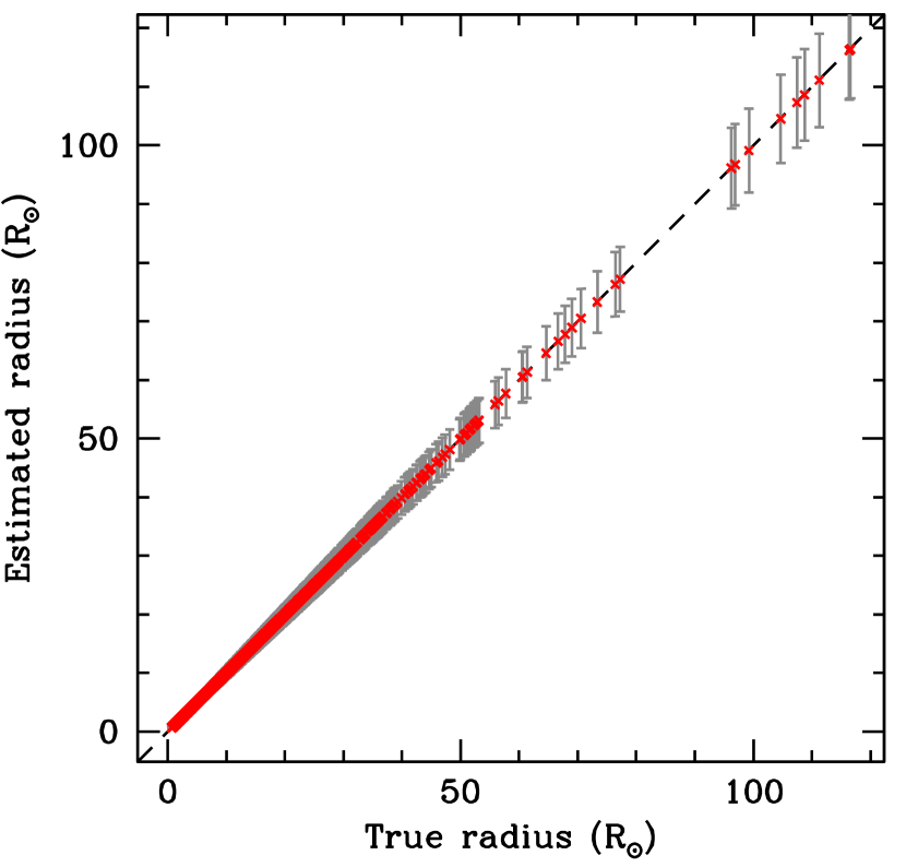
Figure 1: Radius of simulated stars obtained $\Delta\nu$, $\nu_{\rm max}$ and $T_{\rm eff}$ using Equations (1) and (2). No errors were added to the data. The gray errorbars show what the errors would be assuming a 2.5% error in $\Delta\nu$, 5% error in $\nu_{\rm max}$ and 100K error in $T_{\rm eff}$.

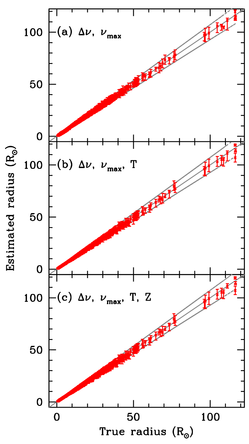
Figure 2: Radius of simulated stars obtained using the grid method using various combinations of seismic and non-seismic data. No errors were added to the data. The points with errorbars show the estimated radii and the errorbars we would have expected for the errors adopted. The middle gray line is where the points would be if the method worked perfectly, while the two other show the $1\sigma$ errors using the “direct” method. Note that the grid method results in somewhat smaller errorbars, but that even for data with no errors, we do not always estimate the radius correctly.

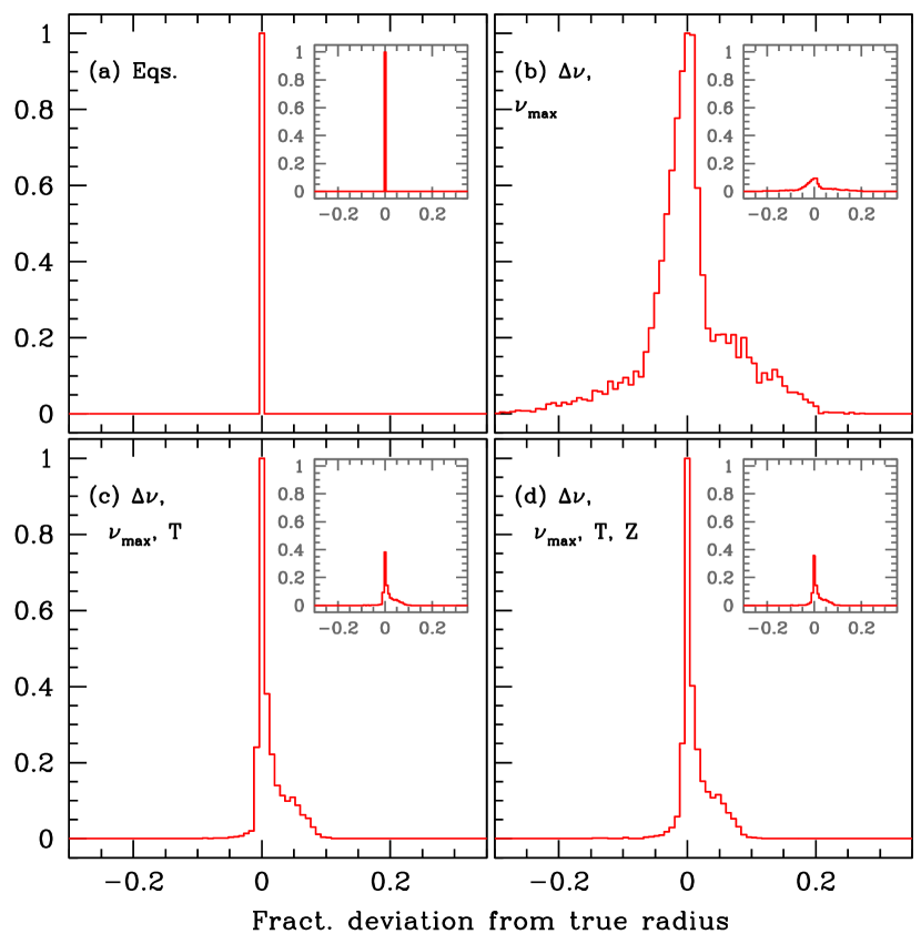
Figure 3: Histograms showing the fractional deviation between the true radii and the radii estimated using different methods to show the accuracy of the methods. These results are for error-free data. All histograms have been normalized to unity at the maximum to facilitate easy comparison of their widths. Panel (a) is the result of the direct method, which as can be seen, gives a perfect results. Panels (b), (c) and (d) are results for the grid method using different combinations of data as mentioned in the figure legends. The inset in each panel shows the distributions normalized to unit area.

We show the result of directly estimating radius using Equations 1 and 2 in Figure 1. These are results for error-free data, however, we also show the error-bars that would result if we had used data with the errors we have adopted. The radius estimates obtained with the grid method, again for error-free data, are shown in Figure 2. These are results obtained with the YREC grid. We show results of using different combinations of inputs. It should be noted that although the input data have no errors, the adopted errors were used to define the volume in the grid within which we calculated the likelihood function. As can be seen, there is some systematic error in the results, in particular at large radii where the estimated radius differs slightly from the true radius. It can be seen that the uncertainties in the results obtained by the grid method will be lower than those obtained by the direct method when inputs that have errors are used. The systematic error is quantified in Figure 3 where we have plotted a normalized histogram of the deviation of the estimated radius from the true radius for each of the four cases shown in Figures 1 and 2.

Note that we have plotted histograms normalized to unity at maximum. While normalizing to unit area emphasizes differences between the distributions (wider distributions have smaller amplitude), it is difficult to estimate visually, and compare, the full-width at half maximum (FWHM) of the distributions. The FWHM of the distributions tells us whether or not the error-distribution is acceptable. Normalizing the distributions to have a maximum value of unity makes the differences between the distributions less obvious. However, it makes determining (and comparing) the FWHM of different distributions much easier. Since it is often conventional to plot histograms normalized to unit area, in each figure we show an inset with the conventional normalization.

As can be seen from Figure 3, the direct method has no systematic error. The systematic errors in the grid method depend on the combination of inputs used, and it is evident that it is important to know $T_{\rm eff}$ in addition to the seismic quantities. The addition of metallicity to the inputs does not appear to make much of a difference.

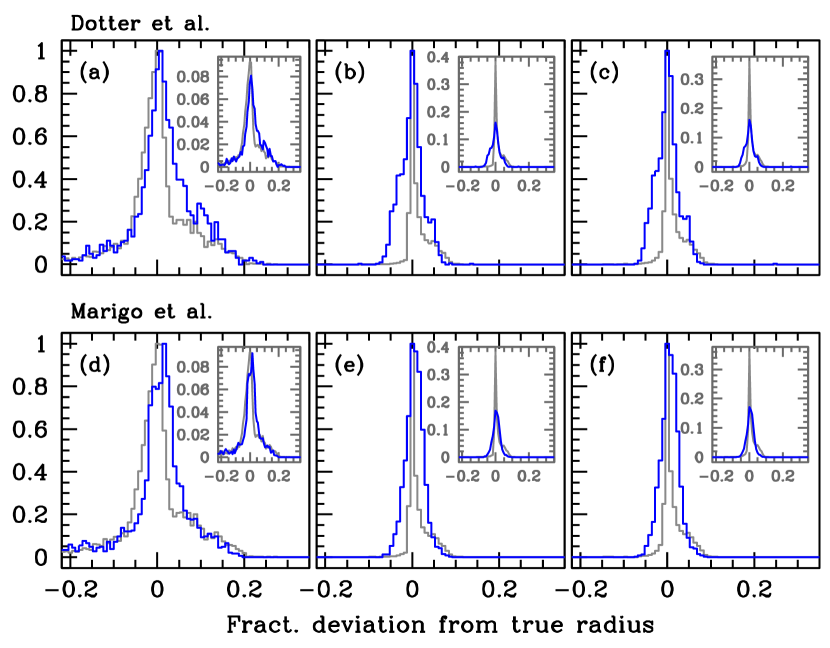
Figure 4: The effect of using a grid constructed with somewhat different physics than the simulated stars (which were all YREC models). As in Figure 3 we show histograms showing the fractional deviation between the true and estimated radii. In blue we show results obtained using the grid of Dotter et al. models (upper row) and the Marigo et al. models (lower row). The histograms in gray show the corresponding results for the YREC grid. Results are for error-free data and show that the effects of known uncertainties in stellar models can lead to systematic errors in the results obtained using the grid method. Panels (a) and (d) are results obtained using $\Delta\nu$ and $\nu_{\rm max}$; panels (b) and (e) are for $\Delta\nu$, $\nu_{\rm max}$, and $T_{\rm eff}$; panels (c) and (f) are results for $\Delta\nu$, $\nu_{\rm max}$, $T_{\rm eff}$and [Fe/H]. The inset in each panel shows the distributions normalized to unit area.

The results described above were obtained for YREC-based stars while using the YREC grid, and hence, a grid with the same physics. In order to test possible systematic errors induced by uncertainties in physics as well as uncertainties in modelling parameters such as the mixing length parameter, we repeated the grid modelling exercise for YREC stars with Dotter et al. and Marigo et al. grids. Again we used error-free data. As mentioned earlier, the Dotter et al. and Marigo et al. models differ considerably from YREC models. The histogram of errors for the radii of YREC stars, as obtained using the two other grids, are shown in Figure 4. As can be seen, the errors in the results are large; however, once $T_{\rm eff}$ is known, the half-width at half-maximum (HWHM) is only about 2.5%, though the largest errors can be about 10%. This error is of the same order as that obtained for the YREC grid when we did not use $T_{\rm eff}$. These results are consistent with our earlier results in Basu et al. (2010) for radius determinations with models with different mixing lengths, however, while we had earlier considered only six cases, two each at the main-sequence, turn-off and sub-giant phases, we have now considered a few thousand of cases with models spanning all evolutionary stages from the zero-age main-sequence to the red-clump.

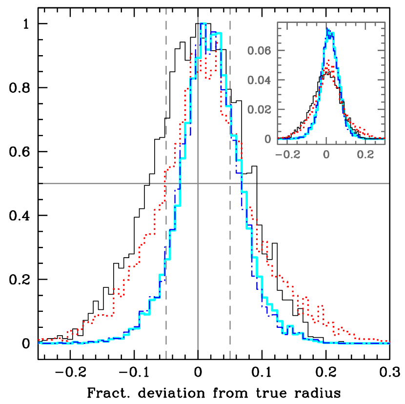
Figure 5: Histograms showing the fractional deviation between the true radii and radii obtained from different methods when errors were added to the data. These histograms show the precision of the method. The results were obtained using the YREC grid. The thin black solid line shows the result of using the direct method. The other lines are for the grid method using different data combinations: the red dotted line shows the result of using only $\Delta\nu$ and $\nu_{\rm max}$; the thick cyan line for $\Delta\nu$, $\nu_{\rm max}$ and $T_{\rm eff}$; and the blue dot-dashed line for $\Delta\nu$, $\nu_{\rm max}$, $T_{\rm eff}$ and $Z$. The solid gray vertical line indicates zero deviation, while the gray dashed lines indicate errors of $\pm 5$%. The grey horizontal line marks the half-maximum of the distributions. The inset shows the distributions normalized to unit area.

Our results give confidence that the grid method works well for estimating the radius, at least where error-free data are concerned. The question, of course, is what happens if data with errors are used. The results for data with our fiducial errors obtained using the YREC grid are shown in Figure 5. Results for about 7300 stars are shown in the histograms. One can see that the direct method gives the worst results. Even if we only use the two seismic parameters $\Delta\nu$ and $\nu_{\rm max}$, the grid method gives better results than the direct method. When $T_{\rm eff}$ and metallicity are also used the HWHM is about 5%. In contrast, the HWHM is about 10% when the direct method is used. While using only $\Delta\nu$ and $\nu_{\rm max}$ in the grid method gives a low HWHM (about 7%), the distribution has substantial tails showing that for individual stars we could get large errors in radius if we only use the two seismic inputs. However, for the nominal errors that we have adopted, the errors we obtain are rarely greater than 20%.

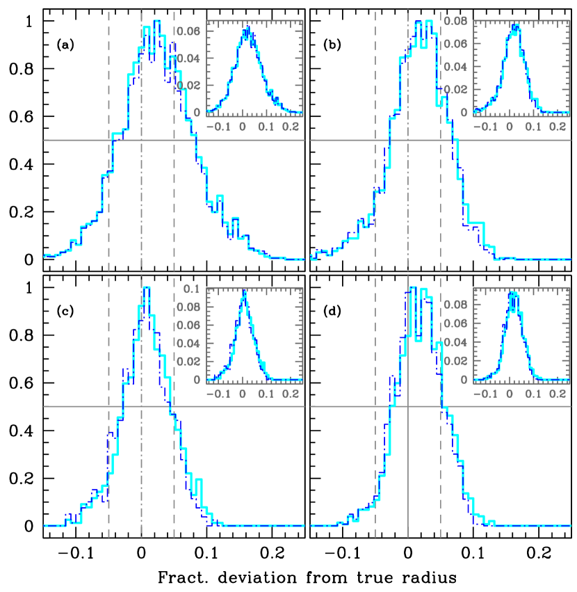
Figure 6: The same as Figure 5, but for stars in selected $\Delta\nu$ ranges. We show results for stars with $\Delta\nu\leq 20\mu$Hz (panel a), $20<\Delta\nu\leq 75\mu$Hz (panel b), $75<\Delta\nu\leq 100\mu$Hz (panel c), and $\Delta\nu>100\mu$Hz (panel d). We only show the grid results using the $(\Delta\nu,\nu_{\rm max},T_{\rm eff})$ combination (thick cyan line) and the $(\Delta\nu,\nu_{\rm max},T_{\rm eff},Z)$ combination (dot-dashed blue line). Only results obtained with YREC data are shown. The inset in each panel shows the distributions normalized to unit area.

How well we can estimate the radius of a star appears to depend on its evolutionary state. In Figure 6 we show the errors in the radius when we split our sample into four groups by $\Delta\nu$. Stars with $\Delta\nu\leq 20\mu$Hz, i.e., giants, give the worst estimates — this result is consistent what we reported in Basu et al. (2010). The best estimates are obtained for stars with $75\leq\Delta\nu<100\mu$Hz.

All distributions of errors obtained for the grid method are asymmetric about the zero point, which reflects the complex non-linear relationship between radius and the observed stellar parameters. With the errors adopted for this work, the figures tell us that we can expect errors in radius estimates caused by errors in the observational inputs to dominate over the systematic errors of the grid method. However, that will not be the case if we can decrease errors in $\Delta\nu$ and $\nu_{\rm max}$ by a much larger amount, an unlikely case for Kepler survey stars. Random errors in temperature have a much smaller effect and are relatively unimportant. And since it is unlikely that we can get metallicity errors to be lower than the adopted value of 0.1 dex, we will probably always be random-error dominated.

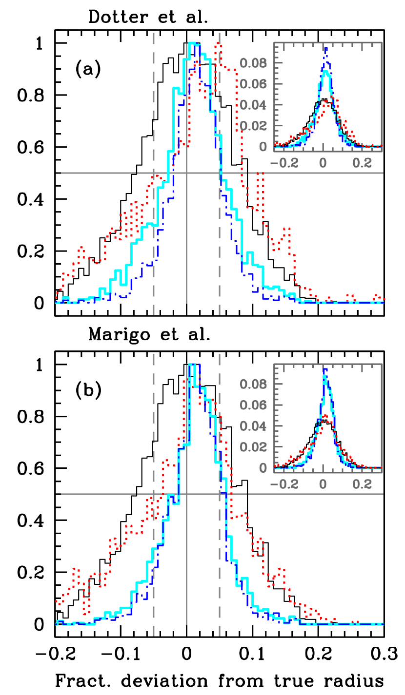
Figure 7: Same as Figure 5 but for results obtained using the grid of Dotter et al. models (panel a) and Marigo et al. models (panel b). The line types are also the same as those in Figure 5.

Using dissimilar grids does change the situation somewhat, in particular, there is a large systematic shift in the results if only the two seismic parameters $\Delta\nu$ and $\nu_{\rm max}$ are used as shown in Figure 7. The systematic shift becomes insignificant when $T_{\rm eff}$ is used and reduces further when metallicity is also used. The HWHM of the error-distribution, however, is comparable to what is obtained with the YREC grid, i.e., about 5%.

Given that 1D stellar models can never simulate real stars, we try out the grid method on solar data using all three grids of models. We used the solar large spacing obtained from solar $\ell=0$ frequencies measured by the Birmingham Solar-Oscillations Network (Chaplin et al. 1996). In particular we use the mode set BiSON-1 described in Basu et al. (2009) to determine an the average large spacing calculated between 2.47 mHz and 3.82 mHz for use as a seismic input parameter. The interval was chosen to be roughly ten large spacings centred around the frequency of maximum power. This choice is prompted by what we can expect from Kepler in the Survey Phase. The errors used were the same as that adopted in this paper. The results are tabulated in Table 1, and as can be seen, we can determine the solar radius quite well. The errors are smallest when we use the combination ($\Delta\nu$, $\nu_{\rm max}$, $T_{\rm eff}$, and $Z$). Since using dissimilar grids simulates some of the uncertainties we may face when we get real data, and since we can reproduce the solar radius well using $\Delta\nu$ and $\nu_{\rm max}$ for the Sun using all three grids, we can be confident about our error estimates.

Table 1: Solar radius (in units of $R_{\odot}$) obtained with BiSON data using different grids and input combinations

Grid	Input combinations
	($\Delta\nu$, $\nu_{\rm max}$)	($\Delta\nu$, $\nu_{\rm max}$, $T_{\rm eff}$)	($\Delta\nu$, $\nu_{\rm max}$, $T_{\rm eff}$, $Z$)
Dotter et al.	$0.978^{+0.020}_{-0.018}$	$1.008^{+0.051}_{-0.062}$	$1.002^{+0.042}_{-0.054}$
Marigo et al.	$1.016^{+0.021}_{-0.016}$	$1.000^{+0.036}_{-0.051}$	$1.001^{+0.035}_{-0.049}$
YREC	$1.016^{+0.021}_{-0.020}$	$0.992^{+0.029}_{-0.050}$	$1.001^{+0.065}_{-0.053}$

3.2 Mass

We have repeated the tests described above for the case of determining masses of stars.

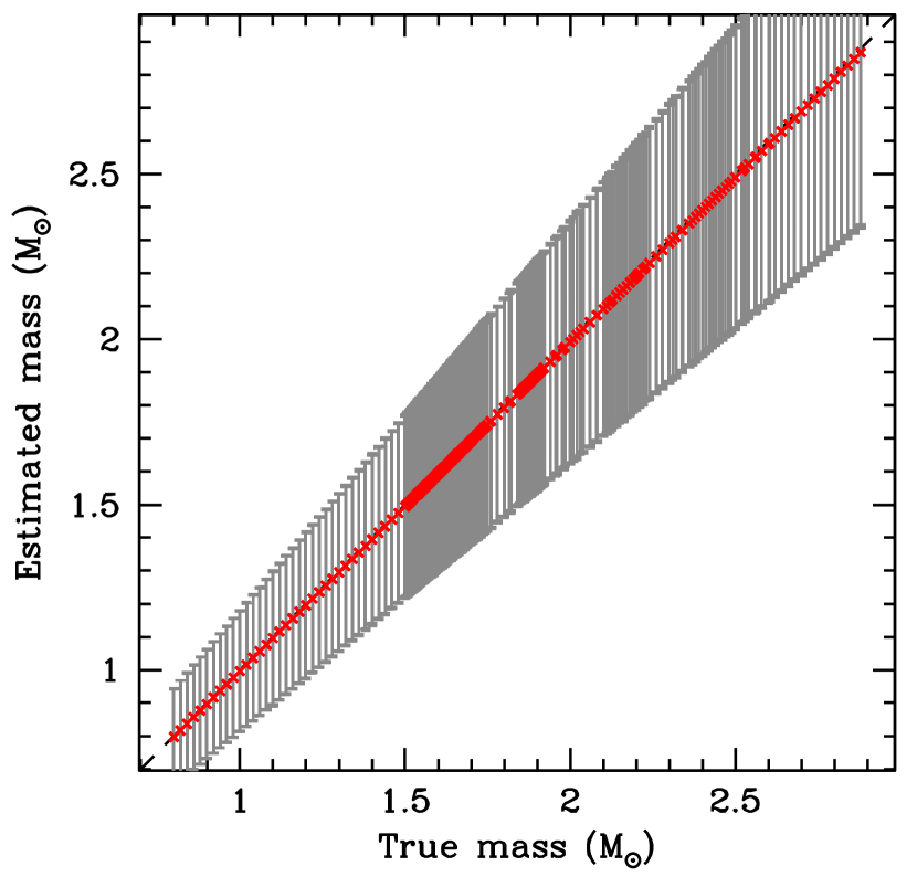
Figure 8: Mass of simulated stars obtained from $\Delta\nu$, $\nu_{\rm max}$ and $T_{\rm eff}$ using Equations (1) and (2). No errors were added to the data. The gray errorbars show what the errors would be for our fiducial errors.

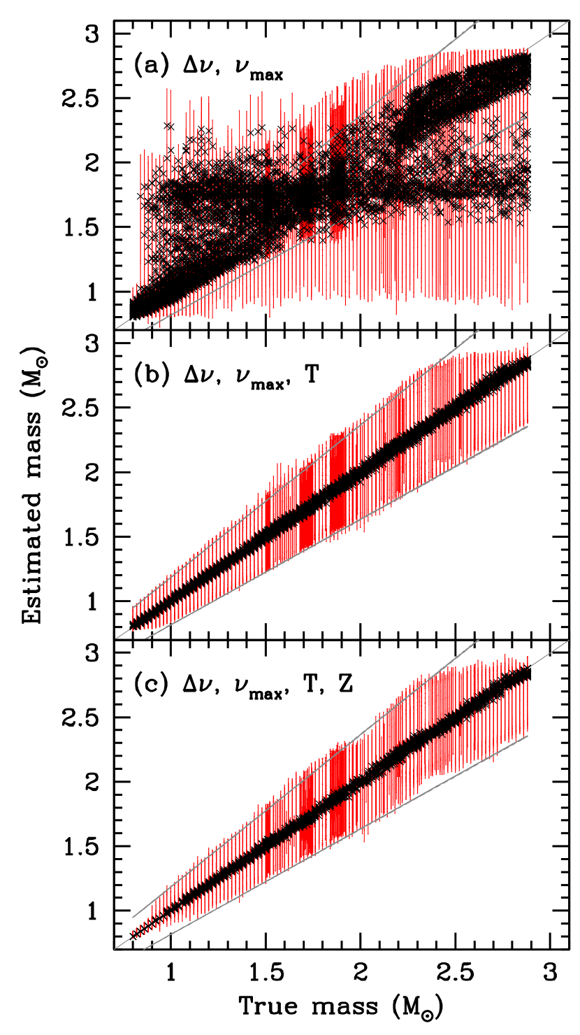
Figure 9: Mass of simulated stars obtained using the grid method. No errors were added to the data. The black points with errorbars show the estimated radii and the errorbars we would have expected for the errors adopted. The middle gray line is where the points would be if the method worked perfectly, while the two other show the $1\sigma$ errors using the “direct” method. All results were obtained with the YREC grid.

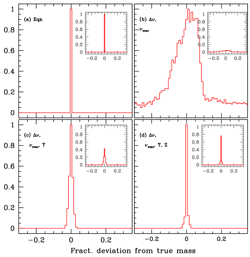
Figure 10: Histograms showing the fractional deviation between the true masses and the masses estimated using different methods to show the accuracy of the methods. These results were obtained using the YREC grid with error-free data. All histograms have been normalized to unity at the maximum to facilitate easy comparison of their widths. Panel (a) is the result of the direct method, which as can be seen, gives a perfect results. Panels (b), (c) and (d) are results for the grid method using different combinations of data as mentioned in the figure legends. The inset in each panel show the distributions normalized to unit area.

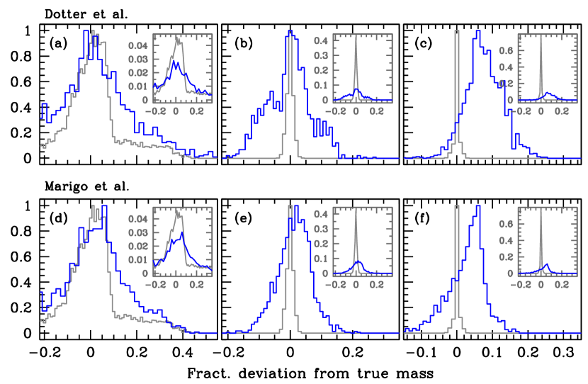
Figure 11: The effect of using a grid constructed with somewhat different physics than the simulated stars (which were all YREC models). In blue we show the histograms of fractional deviation between the true and estimated masses obtained using the grid of Dotter et al. models (upper row) and the Marigo et al. models (lower row). The histograms in gray show the corresponding results for the YREC grid. Results are for error-free data. Panels (a) and (d) are results obtained using $\Delta\nu$and $\nu_{\rm max}$; panels (b) and (e) are for $\Delta\nu$, $\nu_{\rm max}$, and $T_{\rm eff}$; panels (c) and (f) are results for $\Delta\nu$, $\nu_{\rm max}$, $T_{\rm eff}$and [Fe/H]. The insets show the distributions normalized to unit area.

The direct method, as is obvious from Equations (1) and (2), gives much larger error in mass, and this can be seen in Figure 8 where we show the results for the error-free case. The expected errors reduce (but become asymmetric) when the grid method with YREC models is used. The grid results in the error-free case are shown in Figure 9, and we find that unless we know $T_{\rm eff}$, we cannot use the grid method. Also, as far as mass is concerned, the grid method is most useful for the lowest-mass stars, and also stars with somewhat higher masses, particularly if metallicity is known. The error-distributions for the different cases are shown in Figure 10. It is very clear that using only $\Delta\nu$ and $\nu_{\rm max}$ does not work. Again the question is what will happen in the real case. Since we do not have independent mass and seismic measurements of stars other than the Sun, we mimic this case by using a grid of models that are different from the proxy stars. The results are not very promising, as can be seen from Figure 11 and it appears that it is essential that we have good metallicity estimates.

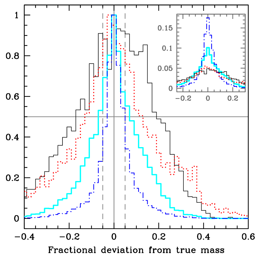
Figure 12: Histograms showing the fractional deviation between the true masses and masses obtained from different methods when errors were added to the data. The thin black solid line shows the result of using the direct method. The other lines are for the grid method using the YREC grid and different data combinations: the red dotted line shows the result of using only $\Delta\nu$ and $\nu_{\rm max}$; the thick cyan line for $\Delta\nu$, $\nu_{\rm max}$ and $T_{\rm eff}$; and the blue dot-dashed line for $\Delta\nu$, $\nu_{\rm max}$, $T_{\rm eff}$ and $Z$. The solid gray vertical line indicates zero deviation, while the gray dashed lines indicate errors of $\pm 5$%. The grey horizontal line marks the half-maximum of the distributions. Note that the distributions are wider than the corresponding distributions for radii (Fig. 5). The inset shows the distributions normalized to unit area.

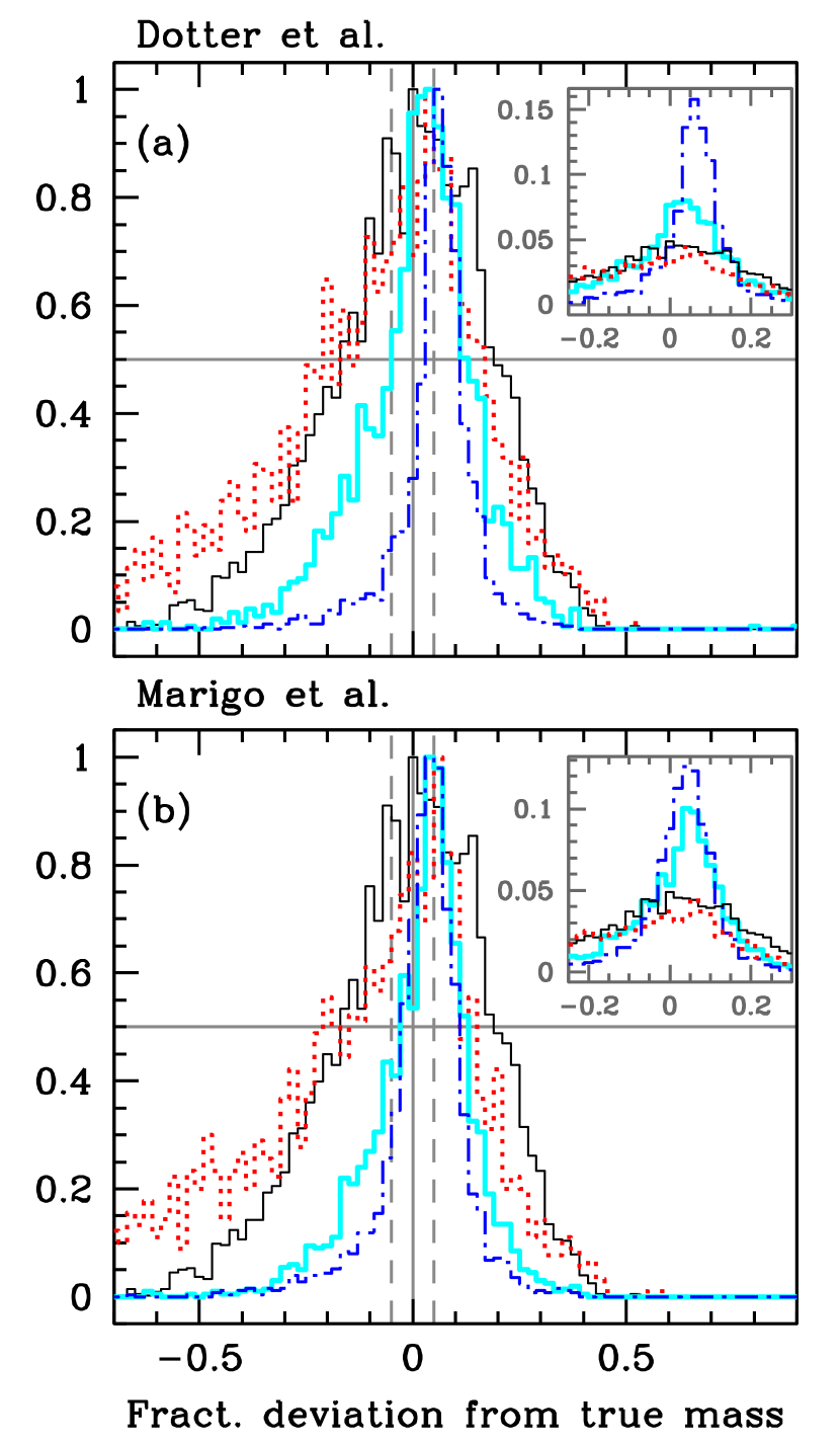
Figure 13: The same as Figure 12 but for results obtained using the grid of Dotter et al. models (panel a) and Marigo et al. models (panel b). The line types are also the same as those in Figure 12.

Despite the seemingly discouraging results, it still appears that in the more realistic case, i.e., when the input data have errors, grid modelling will give better results. The error-distribution for the direct method, and the grid method for three different inputs, is shown in Figure 12 for the YREC grid and in Figure 13 for the Dotter et al. and Marigo et al. grids. It is clear that as long as we know the effective temperature, final errors in the grid modelling will be much better than those in the direct determination case. The results are substantially improved when metallicity is known, with a HWHM of around 5%. Solar mass estimates using the different grid are listed in Table 2, and we do indeed get the best results if we explicitly use the knowledge of metallicity.

Table 2: Solar mass (in units of $M_{\odot}$) obtained with BiSON data using different grids and input combinations

Grid	Input combinations
	($\Delta\nu$, $\nu_{\rm max}$)	($\Delta\nu$, $\nu_{\rm max}$, $T_{\rm eff}$)	($\Delta\nu$, $\nu_{\rm max}$, $T_{\rm eff}$, $Z$)
Dotter et al.	$1.066^{+0.116}_{-0.069}$	$1.025^{+0.125}_{-0.225}$	$1.000^{+0.050}_{-0.050}$
Marigo et al.	$1.032^{+0.066}_{-0.074}$	$1.004^{+0.094}_{-0.130}$	$1.012^{+0.066}_{-0.062}$
YREC	$1.067^{+0.057}_{-0.171}$	$1.002^{+0.183}_{-0.152}$	$1.027^{+0.052}_{-0.060}$

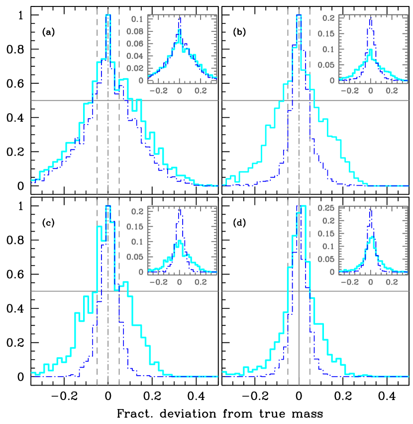
Figure 14: The same as Figure 12, but for stars in selected $\Delta\nu$ ranges. We show results for stars with $\Delta\nu\leq 20\mu$Hz (panel a), $20<\Delta\nu\leq 75\mu$Hz (panel b), $75<\Delta\nu\leq 100\mu$Hz (panel c), and $\Delta\nu>100\mu$Hz (panel d). We only show the grid results using the $(\Delta\nu,\nu_{\rm max},T_{\rm eff})$ combination (thick cyan line) and the $(\Delta\nu,\nu_{\rm max},T_{\rm eff},Z)$ combination (dot-dashed blue line). The inset in each panel shows the distributions normalized to unit area.

As in the case of radius, it is easier to find masses of stars that are either on or close to the main-sequence than it is for red-giants. Error-distributions of mass estimates obtained in different ranges of $\Delta\nu$ are shown in Figure 14. Only results obtained with the YREC grid are shown.

3.3 Error correlations and $\log g$

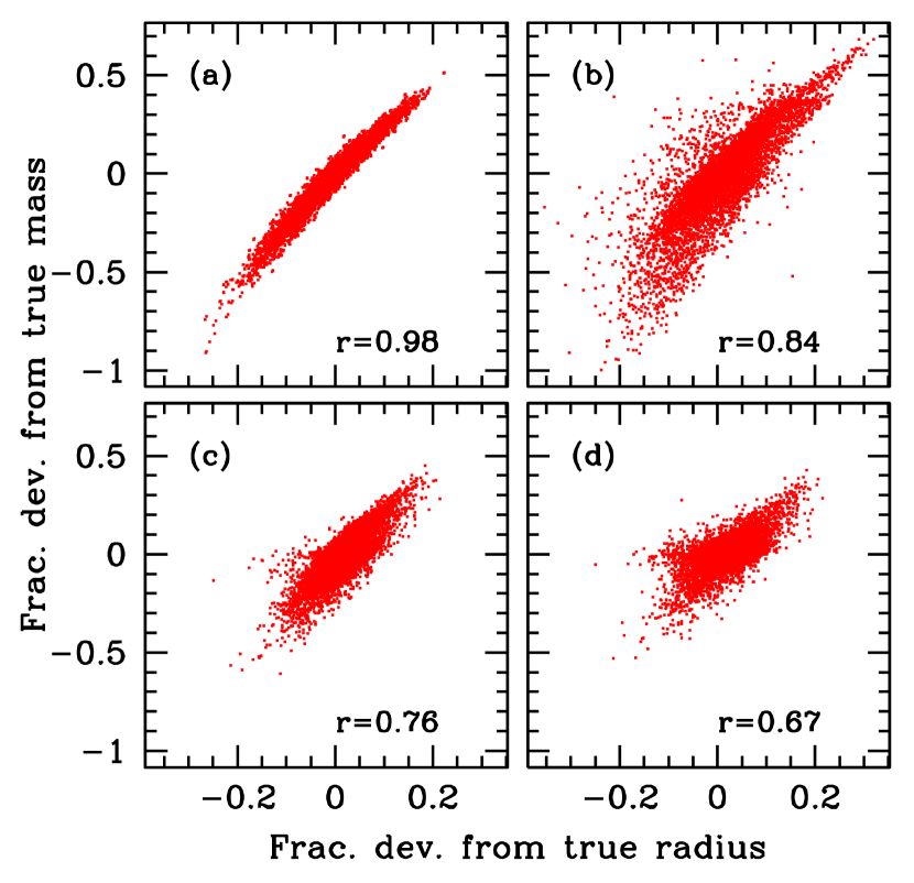
Figure 15: The correlation between errors in estimated mass and radius as given by different methods. The linear correlation coefficient in each case is mentioned in the figure. Panel (a) is the result of the direct method, which, as can be seen, gives perfect results. Panels (b), (c) and (d) are results for the grid method using different combinations of data as mentioned in the figure legends: panel (b) for $(\Delta\nu,\nu_{\rm max})$, panel (c) for $(\Delta\nu,\nu_{\rm max},T_{\rm eff})$ and panel (d) for $(\Delta\nu,\nu_{\rm max},T_{\rm eff},Z)$. Only results obtained with YREC grid are shown.

We expect errors in mass and radius to be correlated. In the direct method the two quantities are determined from the same two equations, and in the grid method they are determined from the same population of models. While we can expect the errors to be almost completely correlated for the direct method, the expected correlation is less obvious for the grid method. To determine the extent of the correlations we have plotted the fractional deviation from true mass against the fractional deviation from true radius for the nearly 7300 simulated stars. The results are shown in Figure 15. The errors are positively correlated. The linear correlation coefficient is noted in each panel and as can be seen, the correlation is substantial even in the grid modelling case. Thus, we need to keep in mind that if we underestimate the radius, we will also underestimate the mass of the star in question.

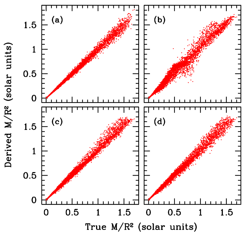
Figure 16: The ratio $M/R^{2}$ derived from estimated values of mass and radius and plotted as a function of the true value. The results indicate that we should be able to estimate $\log g$ accurately. Panel (a) is the result of the direct method, which, as can be seen, gives perfect results. Panels (b), (c) and (d) are results for the grid method using different combinations of data as mentioned in the figure legends: panel (b) for $(\Delta\nu,\nu_{\rm max})$, panel (c) for $(\Delta\nu,\nu_{\rm max},T_{\rm eff})$ and panel (d) for $(\Delta\nu,\nu_{\rm max},T_{\rm eff},Z)$.

The positive correlation between the mass and radius pointed us to the fact that errors in functions involving the ratio of $M$ and $R$ may be smaller. From Figure 15 it can be seen that when the deviation of mass is plotted against the deviation of radius, we do not get a completely straight line but a somewhat curved relation and since $M/R$ is not an observed physical quantity, we investigate $M/R^{2}$, i.e., $g$, instead. In Figure 16 we plot the value of $M/R^{2}$ derived from $M$ and $R$ estimated separately with the true value of $M/R^{2}$ and find that regardless of the method, or of the combination of inputs to the grid method, we get a tight straight line. We, therefore, believe that we should be able to estimate $\log g$ of stars very well.

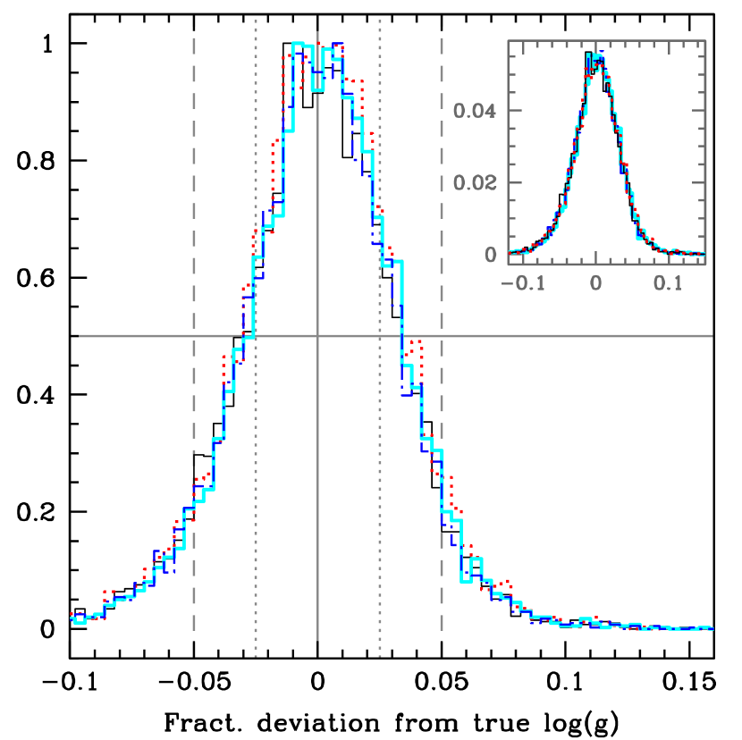
Figure 17: Histograms showing the fractional deviation between true $\log g$ and $\log g$ obtained from different methods using the YREC grid when errors were added to the data. The thin black solid line shows the result of using the direct method. The other lines are for the grid method using different data combinations: the red dotted line shows the result of using only $\Delta\nu$ and $\nu_{\rm max}$; the thick cyan line for $\Delta\nu$, $\nu_{\rm max}$ and $T_{\rm eff}$; and the blue dot-dashed line for $\Delta\nu$, $\nu_{\rm max}$, $T_{\rm eff}$ and $Z$. The solid gray vertical line indicates zero deviation, while the gray dashed lines indicate errors of $\pm 5$%, the dotted gray lines represent $\pm 2.5$% error and the grey horizontal line marks the half-maximum of the distributions. The inset shows the distributions normalized to unit area.

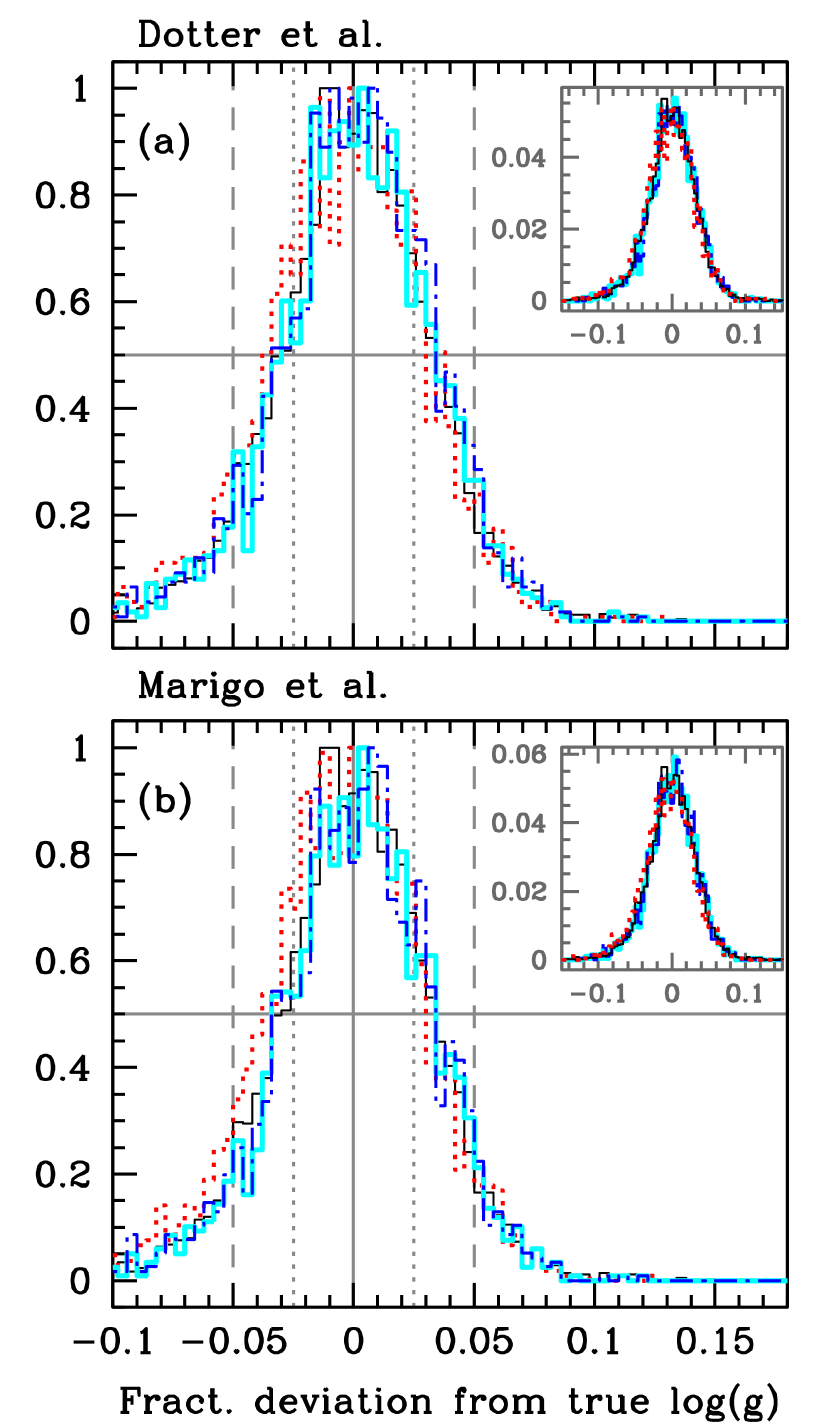
Figure 18: The effect of dissimilar models on $\log g$ estimates. The line types are the same as in Figures 7 and 13. The additional dotted gray lines represent $\pm 2.5$% error.

The error-histograms for $\log g$ determined by different methods, using the YREC grid, are shown in Figure 17 and with the Marigo et al. and Dotter et al. grids are shown in Figure 18. We only show the case where the input quantities had errors added. As can be seen, all methods give almost equally good results and when similar models are used the HWHM is only 2.5%. The error is slightly larger (HWHM about 3.5%) when dissimilar models are used.

As with radius and mass, we have used BiSON data to estimate $\log g$ for the Sun. The results are listed in Table 3. As expected from the discussion above, we get good results no matter which input combination we use.

Table 3: Sun’s $\log g$ obtained with BiSON data using different grids and input combinations. Note that the accepted value of solar $\log g$ is 4.438.

Grid	Input combinations
	($\Delta\nu$, $\nu_{\rm max}$)	($\Delta\nu$, $\nu_{\rm max}$, $T_{\rm eff}$)	($\Delta\nu$, $\nu_{\rm max}$, $T_{\rm eff}$, $Z$)
Dotter et al.	$4.447^{+0.016}_{-0.014}$	$4.438^{+0.018}_{-0.021}$	$4.437^{+0.013}_{-0.011}$
Marigo et al.	$4.442^{+0.011}_{-0.012}$	$4.436^{+0.016}_{-0.016}$	$4.438^{+0.014}_{-0.015}$
YREC	$4.444^{+0.012}_{-0.016}$	$4.434^{+0.016}_{-0.016}$	$4.443^{+0.014}_{-0.013}$

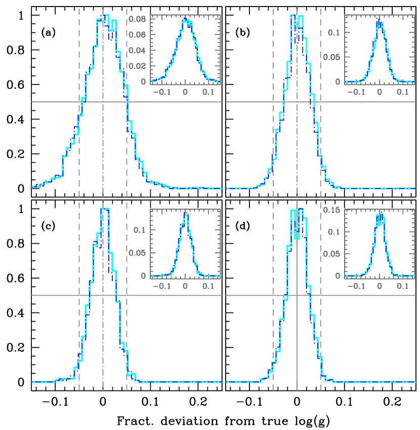
Figure 19: The same as Figures 19, but but for stars in selected $\Delta\nu$ ranges. We show results for stars with $\Delta\nu\leq 20\mu$Hz (panel a), $20<\Delta\nu\leq 75\mu$Hz (panel b), $75<\Delta\nu\leq 100\mu$Hz (panel c), and $\Delta\nu>100\mu$Hz (panel d). We only show the grid results using the $(\Delta\nu,\nu_{\rm max},T_{\rm eff})$ combination (thick cyan line) and the $(\Delta\nu,\nu_{\rm max},T_{\rm eff},Z)$ combination (dot-dashed blue line).

As with mass and radius, $\log g$ is easier to obtain for some stars than for others. The error histograms for stars with different $\Delta\nu$ ranges are shown in Figure 19. As can be seen, errors in $\log g$ are smaller for large $\Delta\nu$ stars (which are large $\log g$ stars too) than for small $\Delta\nu$ stars (which happen to be small $\log g$ stars). However, in all cases the HWHM of the distributions is less than 5%. The quantity $\log g$ is difficult to determine precisely using spectroscopy. Errors can be large, typically 0.1 dex. For instance for Kepler star KIC 11026764 different groups, using the star’s spectrum, find $\log g$ values ranging from $3.84\pm 0.10$ to $4.19\pm 0.16$ (Metcalfe et al. 2010). The uncertainties in $\log g$ from seismology are thus many times smaller than those obtained spectroscopically. Thus it appears that seismology might provide the cleanest way to determine $\log g$.

3.4 Age

Determining stellar ages is crucial for studies of stellar and galactic evolution. The way this is normally done is to fit theoretical evolutionary sequences (e.g. Edvardsson et al. 1992; Ng & Bertelli 1992; Pont & Eyers 2004, etc.) or theoretical isochrones particularly in the case of star cluster (first attempted by Demarque & Larson 1964 and followed by many others). The approach works reasonably well for star clusters as long as the color-magnitude diagram is well defined and stars in all stages of evolution, in particular, the main-sequence, the main-sequence turnoff and the red-giant branch, are present. A similar approach is also used for individual stars, and theoretical tracks are interpolated to the observed parameters of a given star. Pont & Eyer (2004, 2005) have quantified some of the biases that hamper determination of stellar ages. Pont & Eyer (2005) claim that the traditional isochrone ages for field stars are subject to a large systematic bias that they call ‘terminal age bias’, which tends to pull all ages towards the end-of-main-sequence lifetime. This is believed to be a result of the interaction of the observational uncertainties with the strongly varying speed of evolution of stars in the temperature-luminosity diagram. They claim that more sophisticated statistical treatments, particularly Bayesian estimates, are needed to get unbiased ages. Jørgensen & Lindegren (2005) and Takeda et al. (2007) also developed Bayesian-based approaches to determine the ages of individual field stars. Of these, Jørgensen & Lindegren’s approach is very similar to our grid approach, especially since the likelihood function we define can be modified to include any prior.

The two easily observed asteroseismic quantities, $\Delta\nu$ and $\nu_{\rm max}$, do not contain any explicit dependence on age. Age estimates using these two quantities thus rely on what models predict about how $\Delta\nu$ and $\nu_{\rm max}$ change with age. And hence, unlike radius and $\log g$, we know from the very outset that we cannot get model-independent age estimates. The question is how large the model dependence is, and whether we can do any better than non-seismic estimates. Non-seismic estimates rely on measurements of temperature, metallicity and luminosity. Most field stars do not have distance measurements and hence luminosity is difficult to determine. Once we have $\Delta\nu$ and $\nu_{\rm max}$, we do not need to know luminosity since the two seismic quantities contain mass and radius. Prior knowledge of luminosity would, of course, make the age estimates more precise.

It should be noted that model-dependent ages of individual stars can be determined to extremely high precision once frequencies of a reasonable number of individual modes are known (see e.g., Metcalfe et al. 2010). We will not be able to get robust estimates of individual frequencies for all the Kepler stars, hence it is important to be able to test determination of ages using $\Delta\nu$ and $\nu_{\rm max}$. It should also be noted that precise (but again model dependent) ages of main sequence stars can be determined if the so-called small frequency separation $\delta\nu$ is known. This quantity varies with the central hydrogen abundance, and hence age, of a star. Christensen-Dalsgaard (1988) suggested that a plot of $\delta\nu$ against $\Delta\nu$ can be used to determine stellar ages. Modifications to this so-called ‘JCD diagram’ have been suggested by Mazumdar (2005) and Tang et al. (2008). However, this method does not work for more evolved stars (White et al., in preparation). We therefore rely just on $\Delta\nu$ and $\nu_{\rm max}$ for this analysis.

Since Equations (1) and (2) do not contain time explicitly, there is, as noted above, no direct method to determine age. Our preliminary investigations with the grid method have shown that unlike the cases of radius, $\log g$, and mass, we cannot get any estimate of age using $\Delta\nu$ and $\nu_{\rm max}$ alone. Hence we try only two sets of inputs — ($\Delta\nu$, $\nu_{\rm max}$, $T_{\rm eff}$) and ($\Delta\nu$, $\nu_{\rm max}$, $T_{\rm eff}$, [Fe/H]).

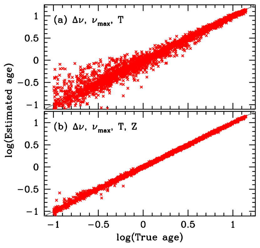
Figure 20: Age estimates (in Gyr) obtained by the grid method using two different data combinations. No errors were added to the data. Both the “stars” and the grid were based on YREC models.

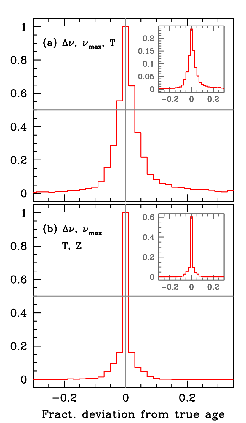
Figure 21: Histograms showing the fractional deviation between the true ages and the ages estimated by the grid method using YREC models to illustrate the accuracy of the determinations for error-free data. The horizontal gray line is the half-maximum, and the vertical gray line indicates accurate results. As with other figures, the inset in each panel shows the distributions normalized to unit area.

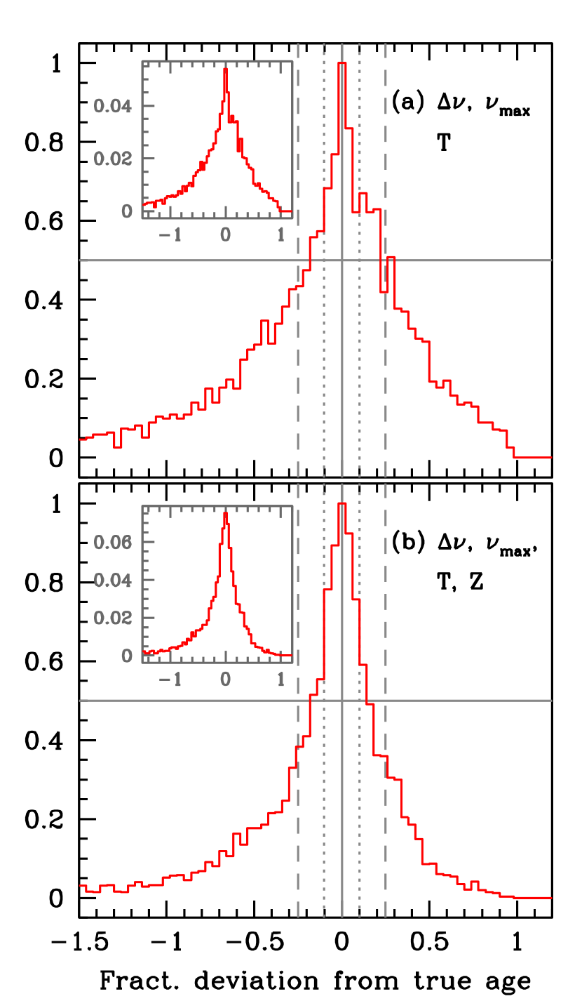
Figure 22: The same as Figure 21 but for the case when errors were added to data. The dashed gray line shows $\pm 25$% error in results, the dotted gray lines mark $\pm 10$% error.

Figure 20 shows the result of estimating the ages of about 7300 stars with error-free data. The stars are based on YREC models, and the results were obtained using the YREC grid. As can be seen, even with a similar grid and error-free data, knowledge of $Z$ is a must. This is not surprising, since stars of the same mass evolve at different rates depending on their metallicity. The error histograms for these cases are shown in Figure 21. The figure shows that using metallicity reduces the HWHM of the distribution from about 5% to less than 2.5% and the maximum error is reduced to 10%. Adding errors to the inputs of course makes the situation worse. The error histograms for this case are shown in Figure 22. Without metallicity, the HWHM is about 20% and the distribution has a large tail. Once metallicity is used, the HWHM reduces to around 15%, and while the distribution still has a long tail, it is not as wide as it was earlier.

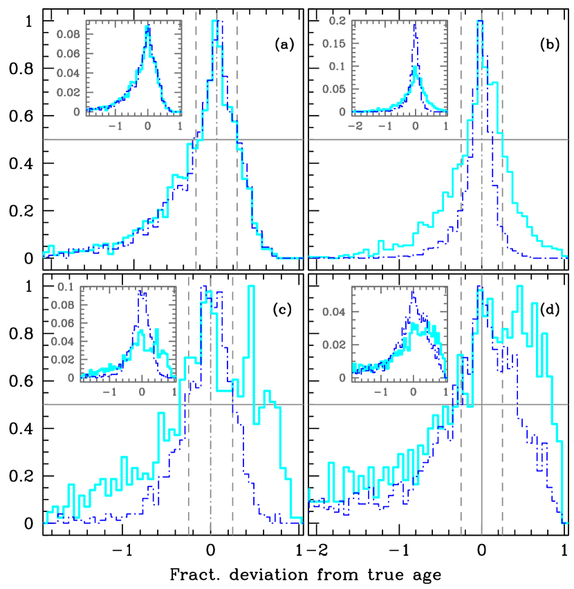
Figure 23: The same as Figure 22, but for stars grouped into different $\Delta\nu$ ranges. The thick cyan line shows the result of using ($\Delta\nu$, $\nu_{\rm max}$, $T_{\rm eff}$) as inputs, the blue dot-dashed lines are the results of using ($\Delta\nu$, $\nu_{\rm max}$, $T_{\rm eff}$, [Fe/H]) as inputs. The solid gray vertical line is for zero deviation, while the dashed lines show $\pm 25$% error. We show results for stars with $\Delta\nu\leq 20\mu$Hz (panel a), $20<\Delta\nu\leq 75\mu$Hz (panel b), $75<\Delta\nu\leq 100\mu$Hz (panel c), and $\Delta\nu>100\mu$Hz (panel d). The inset in each panel shows the distributions normalized to unit area.

As in the cases of radius, mass and $\log g$, we repeated the analysis after grouping stars in $\Delta\nu$ and the results are shown in Figure 23. It appears that using this method, we can find ages of sub-giants and red-giants more precisely than ages of main sequence and turnoff stars. In retrospect, this is not surprising – the rapid variation of stellar radius with age for evolved stars implies a large change in both $\Delta\nu$ and $\nu_{\rm max}$  making this method more sensitive. Thus for main-sequence and turn-off stars, we really need the small-separations to get relatively precise estimates of age. The case of core helium burning red-clump stars is interesting. Errors in temperature and metallicity usually means that the grid method include stars from the ascending part of the red-giant branch in the likelihood function calculations. The converse is also true, the likelihood function of stars on the ascending part of the red-giant branch can include red-clump stars. This results in age-errors that are larger than those for subgiant stars.

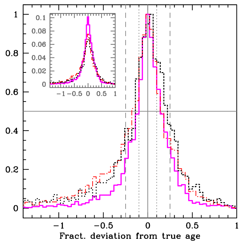
Figure 24: A comparison of histograms showing the fractional deviation between the true ages and the ages obtained using combinations of seismic and non-seismic data with that for non-seismic data only. The dotted black line is for results obtained using only the non-seismic parameters $(T_{\rm eff},Z,M_{v})$, red dot-dashed for $(\Delta\nu,\nu_{\rm max},T_{\rm eff},Z)$ and the magenta solid line for $(\Delta\nu,\nu_{\rm max},T_{\rm eff},Z,M_{v})$. The dashed gray line shows $\pm 25$% error in results, the dotted gray lines mark $\pm 10$% error. The inset shows the distributions normalized to unit area.

An important question is whether using seismic data actually helps us at all. In Figure 24 we show the error histogram for the seismic case with inputs ($\Delta\nu$, $\nu_{\rm max}$, $T_{\rm eff}$, [Fe/H]) and compare it with that of a non-seismic case with inputs ($T_{\rm eff}$, [Fe/H], and $M_{V}$), where we have assumed errors of 0.1 mag in $M_{V}$. The figure confirms our earlier assertion that the information contained in $\Delta\nu$ and $\nu_{\rm max}$ allows us to get comparable error estimates without knowing the luminosity of the stars. If we knew luminosity as well as $\Delta\nu$ and $\nu_{\rm max}$, we would do much better, as we also show in Figure 24.

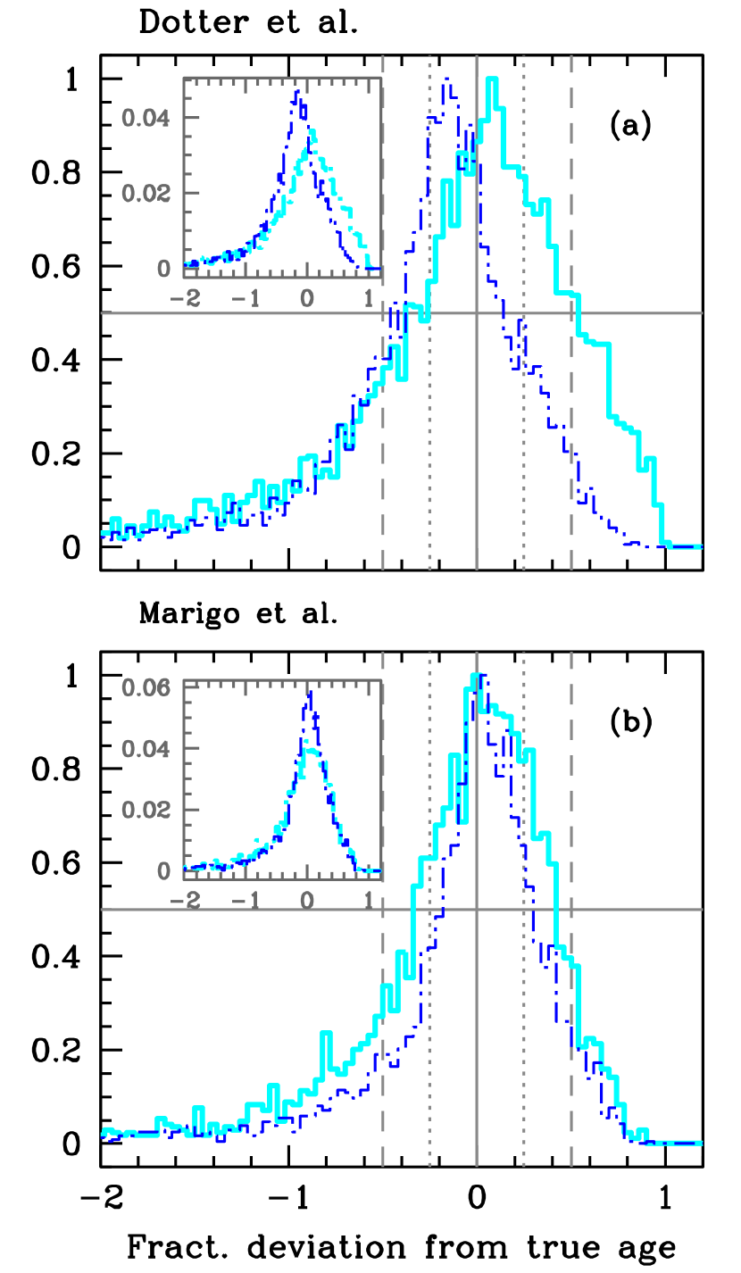
Figure 26: The same as Figure 25 but for the case with errors added to the data.

All the age results are, of course, model dependent. This is shown in 25 for the error-free case where we plot the error histograms for ages obtained with the Marigo et al. and Dotter et al. grid. As expected, the error is larger, and the case for needing metallicity is stronger, with the HWHM being about 20%. In Figure 26 we show what happens when errors are added. As with the other global parameters, it appears that input errors can dominate over the systematic errors. And the figures drive home the need for good metallicity measurements to derive ages properly. The model dependence and uncertainties of the method are demonstrated using solar data. Estimates of the solar age are listed in Table 4. We can see that unless we use metallicity, the error-bars are large enough to make the results essentially useless. Even when we use metallicity, the errors are large, though the central value is more acceptable.

Table 4: The solar age obtained with BiSON data using different grids and input combinations.

Grid	Input combinations
	($\Delta\nu$, $\nu_{\rm max}$, $T_{\rm eff}$)	($\Delta\nu$, $\nu_{\rm max}$, $T_{\rm eff}$, $Z$)
Dotter et al.	$2.96^{+5.57}_{-1.15}$	$4.62^{+2.13}_{-1.73}$
Marigo et al.	$3.98^{+6.02}_{-3.63}$	$3.55^{+2.80}_{-2.75}$
YREC	$5.57^{+6.04}_{-5.05}$	$3.97^{+2.07}_{-1.84}$

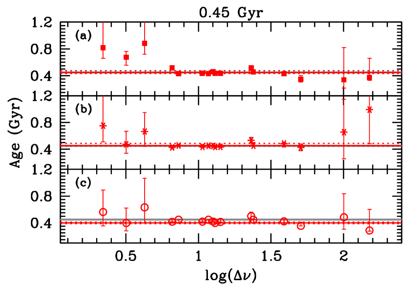
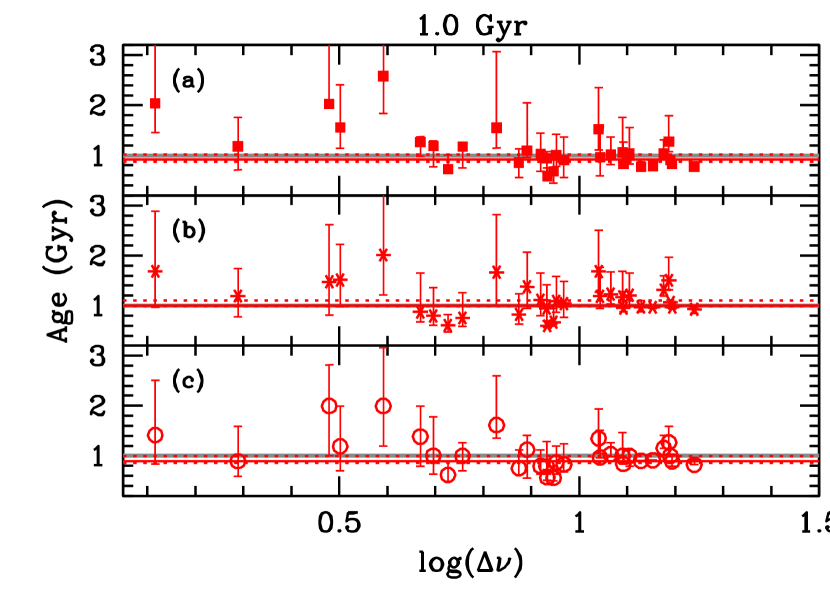
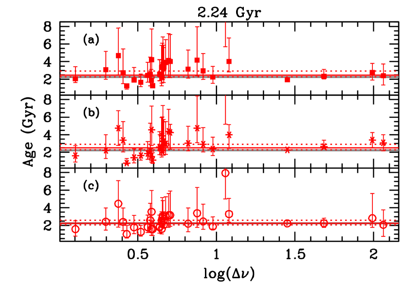
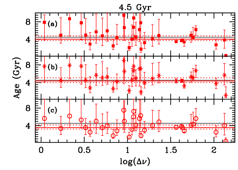
Figure 27: Age results obtained for star clusters. Each main panel shows the result from a simulated cluster of a given age. Sub-panel (a) shows results obtained with the YREC grid, (b) with the Dotter et al. grid and (c) with the Marigo et al. grid. In each sub-panel, the horizontal line marks the true age of the cluster, the points with the error bars are the results for each individual star. The red solid line is the result obtained assuming that all stars in the cluster have the same age, while the dotted lines show the $1\sigma$ error bars on that result.

The Kepler field-of-view contains four open clusters, including NGC 6791 and NGC 6819. Thus the question arises whether we can apply the grid method to determine ages of clusters with the handful of stars that are expected to show detections of solar-like oscillations. Clusters provide two advantages: we can apply the prior that all stars have the same age; and, given the intrinsic interest in clusters, they usually have good metallicity estimates. To determine cluster ages, we first determine the ages of the individual stars, which allows us to remove outliers, and then we re-derive the age of the cluster as a whole after applying the prior that the stars have the same age. The results for four simulated clusters are shown in Figure 27. Two of the clusters were derived from the Dotter et al. grid and two from the Marigo et al. grid, and we derive the ages using all three grids. For each we have between 20 and 30 stars, which is what we expect for initial Kepler data on clusters. We used stars that populate all parts of the color-magnitude diagram, from the main sequence to the red-clump. As can be seen from the figure, it is possible to get precise results for clusters, even with a handful of stars. There are systematic errors though, that result from the differences in the physics and more importantly composition differences between the proxy stars and the grid used. Thus it is extremely important to that before determining ages we first construct a grid of models that correspond to the composition of the cluster.

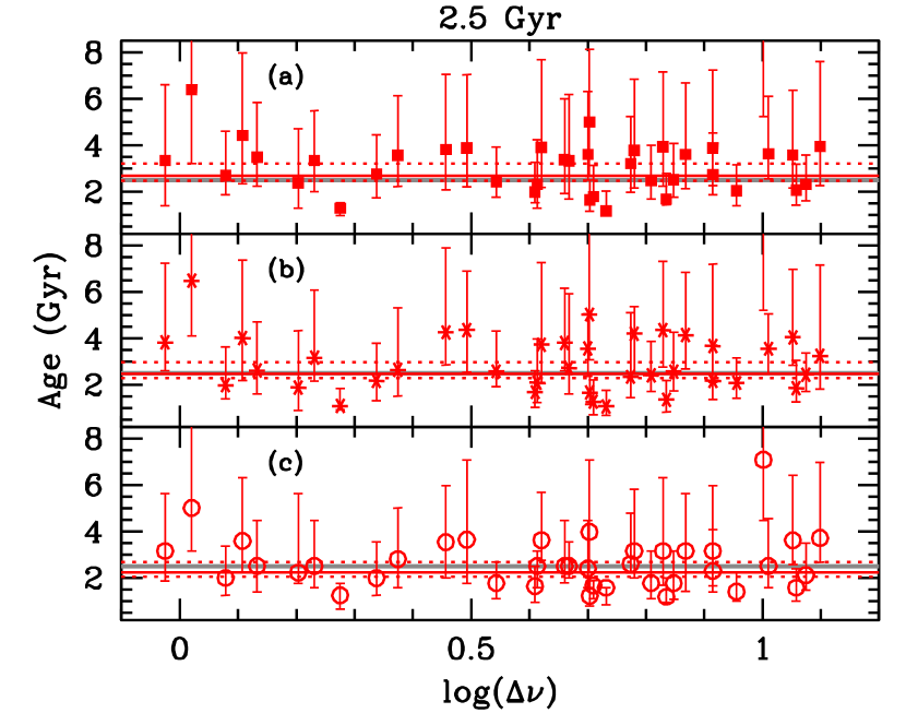
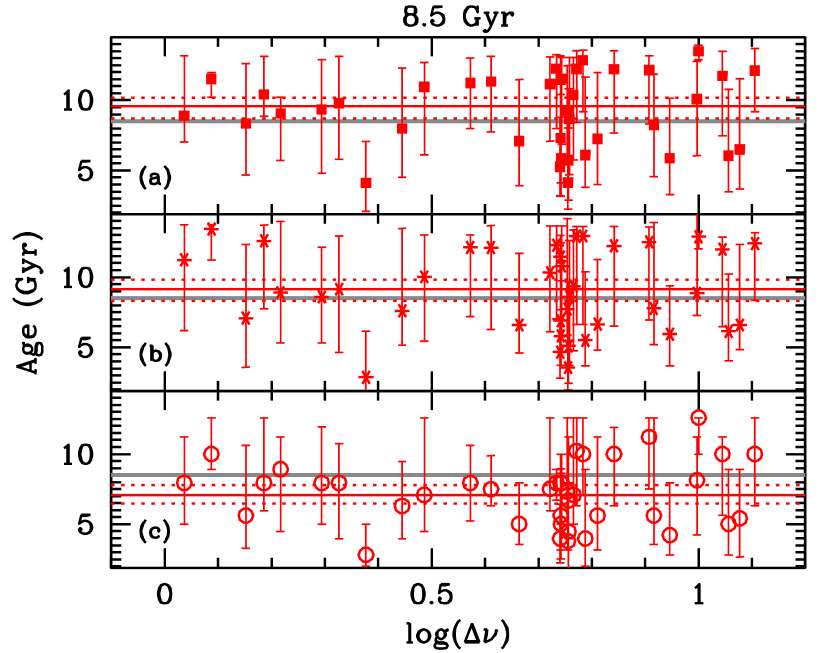
Figure 28: Same as Figure 27, but for the case when only data on red giants and red-clump stars are available. The upper panel has stars of an age similar to that of NGC 6819, the lower panel has stars with age similar to NGC 6791.

Initial data for NGC 6791 and NGC 6819 will only be for red-giants and core helium burning red-clump stars. We know from Figure 23 that having only giants will not be a handicap. However, we test this by simulating a cluster of age 2.5 Gyr (roughly the age of NGC 6891) and one of 8.5 Gyr (around the age of NGC 6791) and use only red-giant and clump stars. The results are shown in Figure 28. As can be seen, we expect precise results for both clusters (with the older cluster having a larger systematic error). It should be noted that these results are independent of the distance-modulus of the clusters. They will depend on the extinction, through temperatures. In addition to ages, we can give model-independent estimates of the distances to the clusters by determining the radii and masses from the seismic data.

4 Conclusions

We made an in-depth study of grid-based asteroseismic analysis to determine possible systematic and other errors in radius and mass estimates derived using seismic data.

We find that when errors in the seismic parameters and $T_{\rm eff}$ are included, error estimates in radius and mass are higher when determined directly from the equations defining the seismic quantities $\Delta\nu$ and $\nu_{\rm max}$ than when determined using the grid method. This is not surprising. Equations (1) and (2) assume that all values of $T_{\rm eff}$ are possible for a star of a given mass and radius. However, the equations of stellar structure and evolution tell us otherwise — we know that for a given mass and radius, only a narrow range of temperatures are allowed. The grid method takes this into account implicitly since the grid is constructed by solving the equations of stellar structure and evolution.

However, grid based asteroseismology can lead to some model dependence. While there is almost no model dependence in derived values of radius, there can be considerable model dependence in mass, unless we have reasonable measures of metallicity. However, given the expected errors in the seismic and non-seismic inputs, the systematic errors are much smaller than the error in the results caused by errors in the observations.

Errors in mass and radius estimates are positively correlated and the correlation is high. The correlation is such that it leads to very small errors in $M/R^{2}$ and hence $\log g$. We find that we can determine $\log g$ precisely and accurately with both direct and grid-based methods and that there is no systematic error in the estimates. Given that $\log g$ estimates from spectroscopy can be extremely imprecise, seismology gives us an alternative to spectroscopy when it comes to determining $\log g$.

Given the near model-independence of the radius and $\log g$ estimates, it may be tempting to assume that we could get near-model independent mass estimates from estimated values of radius and $\log g$. This cannot be done to high precision because although the errors in radius and $\log g$ are small, they get magnified when the error on mass is calculated. Since $M=gR^{2}$, the relative error in mass is, at the very least, the relative error in $g$ and twice the relative error in $R$, added in quadrature. There is a third term that arises from the correlation between $g$ and $R$, which adds to the error in mass. This is not a surprising result since whether we estimate mass on its own or from estimates of radius and $\log g$, the information available is exactly the same.

As far as ages are concerned, seismic data do not give us any direct information, however, since the radius and mass of a star are a function of age, seismic data merely give us two extra pieces of information. Since neither $\Delta\nu$ nor $\nu_{\rm max}$ are explicit functions of age, we can only get model-dependent age estimates. The advantage that seismic data give us is that we do not need to know the distance and absolute luminosity of the star to determine the age through models. The model dependence in the results can be minimized if the abundances of the stars are known. The errors can be rather large, easily as large as 25%. We find however, that we can determine the ages of star clusters to a much higher precision when we apply the prior that all cluster stars have the same age. And unlike isochrone fitting techniques, asteroseismic cluster ages are independent of the distance modulus and can be determined with only a handful of stars. Cluster ages can be determined even if we use only red-giant stars, which is encouraging since initial seismic data from clusters in the Kepler field of view will only be data on the cluster red-giants.

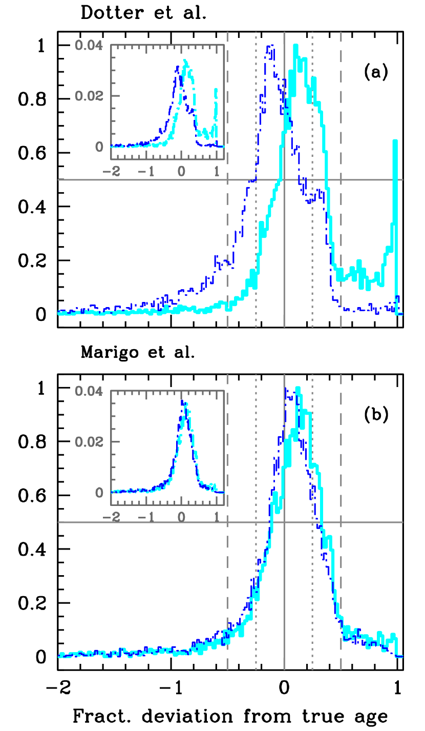
Figure 25: The same as Figure 21 but when a different grid of models was used. Panel (a) shows the results of using the Dotter et al. grid, and panel (b) shows results for Marigo et al. grid. The thick cyan lines are results of using the $(\Delta\nu,\nu_{\rm max},T_{\rm eff})$ combination, and the dot-dashed blue line is for the $(\Delta\nu,\nu_{\rm max},T_{\rm eff},Z)$ combination.

References

- Alexander & Ferguson (1994) Alexander, D. R., Ferguson, J. W. 1994, ApJ, 437, 879
- Angulo et al. (1999) Angulo, C., Arnould, M., Rayet, M., et al. 1999, Nucl. Phys. A., 656, 3
- Basu & Antia (2008) Basu, S., Antia, H. W. 2008, Physics Reports, 457, 217
- Basu et al. (2009) Basu, S., Chaplin, W.J., Elsworth, Y., New, R., Serenelli, A.M., 2009, ApJ, 699, 1403
- Basu et al. (2010) Basu, S., Chaplin, W. J., Elsworth, Y. 2010, ApJ, 710, 1596
- Bedding & Kjeldsen (2003) Bedding, T. R. & Kjeldsen, H. 2003, PASA, 20, 203
- Borucki et al. (2010) Borucki, W. J., Koch, D. G., Basri, G., 2010, Sci, 327, 977
- Chaplin et al. (1996) Chaplin W. J., Elsworth Y., Howe R., Isaak G. R., McLeod C. P., Miller B. A., New R., van der Raay H. B. & Wheeler S. J., 1996, SolPhys, 168, 1
- Chaplin et al. (2008) Chaplin, W. J., Houdek, G., Appourchaux, T., Elsworth, Y., New, R. & Toutain, T. 2008, A&A, 485, 813
- Christensen-Dalsgaard (1988) Christensen-Dalsgaard, J. 1988, in Advances in helio- and asteroseismology, ed. J. Christensen-Dalsgaard, & S. Frandsen (Dordrecht: Reidel), Proc. IAU Symp., 123, 295
- Christensen-Dalsgaard (1993) Christensen-Dalsgaard, J. 1993, in ASP. Conf. Ser. 42, Proc. GONG 1992, Seismic Investigation of the Sun and Stars, ed. T. M. Brown (San Francisco, CA: ASP), 347
- Demarque & Larson (1964) Demarque, P.R., Larson, R.B., 1964, ApJ, 150, 554
- Demarque et al. (2004) Demarque, P., Woo, J. -H., Kim, Y. -C., & Yi, S. K. 2004, ApJS, 155, 667
- Demarque et al. (2008) Demarque, P., Guenther, D. B., Li, L. H., Mazumdar, A. & Straka, C. W. 2008, Ap&SS, 316, 311
- Dotter et al. (2007) Dotter, A., Chaboyer, B., Jevremovic, D. et al. 2007, ApJ, 134, 376
- Dotter et al. (2008) Dotter, A., Chaboyer, B., Jevremovic, D. et al. 2008, ApJ, 178, 89
- Edvardsson et al. (1993) Edvardsson, B., Andersen, J., Gustafsson, B., Lambert, D. L., Nissen, P. E., Tomkin, J., 1993, A&A, 275, 101
- Ferguson et al. (2005) Ferguson, J. W., Alexander, D. R., Allard, F., et al. 2005, ApJ, 623, 585
- Girardi et al. (2000) Girardi, L., Bressan, A., Bertelli, G & Chiosi C., 2000, A&ASS, 141, 371
- Grevesse & Noels (1993) Grevesse, N. & Noels, A. 1993, Phys. Scr. T, 47, 133
- Grevesse & Sauval (1998) Grevesse, N. & Sauval, A. J. 1998, Space Sci. Rev., 85, 161
- Iglesias & Rogers (1993) Iglesias, C. A. & Rogers, F. J. 1993, ApJ, 412, 752
- Iglesias & Rogers (1996) Iglesias, C. A. & Rogers, F. J. 1996, ApJ, 464, 943
- Joergensen & Lindegren (2005) Jørgensen, B. R. & Lindegren, L. 2005, A&A, 436, 127
- Kjeldsen et al. (1995) Kjeldsen, H., Bedding, T. R., Viskum, M. & Frandsen, S. 1995, AJ, 109, 1313
- Lejeune et al. (1997) Lejeune, Th., Cuisinier, F. & Buser, R. 1997, A&A, 125, 229
- Marigo et al. (2008) Marigo, P., Girardi, L., Bressan, A. et al. 2008, A&A, 482, 883
- Mazumdar (2005) Mazumdar, A. 2005, A&A, 441, 1079
- Metcalfe et al. (2010) Metcalfe, T. S., Monteiro, M. J. P. F. G., Thompson, M. J., Molenda-Żakowicz, J., Appourchaux, T., 2010, ApJ, 723, 1583
- Ng & Bertelli (1998) Ng, Y.K., Bertelli, G., 1998, A&A, 329, 943
- Pont & Eyer (2004) Pont, F. & Eyer, L. 2004, MNRAS, 351, 487
- Pont & Eyer (2005) Pont, F. & Eyer, L. 2005, ESASP, 576, 187
- Rogers & Iglesias (2002) Rogers, F. J. & Iglesias, C. A. 1992, ApJS, 79, 507
- Rogers & Nayfovov (2002) Rogers, F. J. & Nayfonov, A. 2002, ApJ, 576, 1064
- Stello et al. (2009) Stello, D., Chaplin, W. J., Bruntt, H. et al. 2009, ApJ, 700, 1589
- Takeda et al. (2007) Takeda, G., Ford, E. B., Sills, A. et al. 2007, ApJ, 168, 297
- Tang et al. (2008) Tang, Y. K., Bi, S. L. & Gai, N. 2008, A&A, 492, L49
- Thoul et al. (1994) Thoul, A. A., Bahcall, J. N. & Loeb, A. 1994, ApJ, 421, 828