Seeing-Induced Errors in Solar Doppler Velocity Measurements

Abstract

Imaging systems based on a narrow-band tunable filter are used to obtain Doppler velocity maps of solar features. These velocity maps are created by taking the difference between the blue- and red-wing intensity images of a chosen spectral line. This method has the inherent assumption that these two images are obtained under identical conditions. With the dynamical nature of the solar features as well as the Earth’s atmosphere, systematic errors can be introduced in such measurements. In this paper, a quantitative estimate of the errors introduced due to variable seeing conditions for ground-based observations is simulated and compared with real observational data for identifying their reliability. It is shown, under such conditions, that there is a strong cross-talk from the total intensity to the velocity estimates. These spurious velocities are larger in magnitude for the umbral regions compared to the penumbra or quiet-sun regions surrounding the sunspots. The variable seeing can induce spurious velocities up to about 1 km s^-1. It is also shown that adaptive optics, in general, helps in minimising this effect.

1 Introduction

S-intro

Recent observations have generated new interest in understanding the sunspot fine structures like umbral dots, light bridges, and penumbral filaments [Rimmele (2008), Rimmele and Marino (2006), Scharmer et al. (2002), Schüssler and Vögler (2006)]. Detailed spatial and temporal observations of these fine structures are crucial in understanding the physical mechanisms behind the formation of these structures. With the success of the solar adaptive optics (AO), it is now feasible to study structures close to the diffraction limit of modern telescopes [Rimmele (2004b), Sankarasubramanian and Rimmele (2003), Sankarasubramanian and Hagenaar (2007), Rimmele (2008)]. These small-scale structures harbour flows that are important for understanding the interaction between magnetic fields and plasma. Observational study of these flows would provide constraints to the theoretical models and to the magnetohydrodynamic simulations of these flows and hence would lead to a better understanding of the overall structure.

Doppler shifts of spectral lines are regularly used to study the line of sight (LOS) velocity of solar features. They are observed either with a spectrograph-based instrument or with an instrument based on tunable narrow-band filter. In instruments based on a tunable narrow-band filter, Doppler velocities are obtained using the red- and blue-wing intensity images of a chosen spectral line. Intensity at a fixed wavelength point in the blue and/or red wing of any spectral line varies depending on the Doppler shift. At a fixed wavelength point in the red wing of an absorption line, a red-(blue-) shift will reduce (increase) the intensity. Similarly, at a fixed point in the blue wing of an absorption line, a red-(blue-) shift will increase (decrease) the intensity. Hence, the difference between the red- and blue-wing intensities obtained at a fixed wavelength point is used to estimate the Doppler shift and hence the Doppler velocity. A magnetic field and its gradients may affect the magnetically sensitive spectral line profiles and hence the Doppler velocities estimated from them [Wachter, Schou, and Sankarasubramanian (2006), Rajaguru et al. (2007)]. Therefore, magnetically insensitive lines are preferred for a “clean” velocity estimation. For example, Fe i 5434 Å or Fe i 5576 Å are typically used to estimate Doppler velocities at the photosphere. Systems based either on a tunable Fabry-Pérot etalon or a universal birefringent filter (UBF) (see ubfreport1975, cavallini2006, stix2002, and references therein for details about these instruments) are used to obtain the required spectral bandwidth (e.g., about 200mÅ for photospheric spectral lines). In both schemes, Doppler velocities are estimated from the difference between intensities obtained at the blue and red wing of a chosen spectral line by using the following relation:

$$V=C.\frac{I_{\rm r}-I_{\rm b}}{I_{\rm r}+I_{\rm b}},\ilabel{eq1}$$ (1)

where $I_{\rm r}$ and $I_{\rm b}$ are the red- and blue-wing intensities and $C$ is a calibration constant which depends on the chosen spectral line and the spectral resolution. $C$ can be obtained using a well-known procedure [Rimmele (2004a)] briefly explained in Section S-simul of this paper. With this definition, positive (negative) velocity correspond to flows towards (away from) the observer. This sign convention is followed throughout this paper.

In such observations, the blue- and red-wing images are NOT recorded simultaneously. The time difference between the two depends on the wavelength tuning time, required number of wavelength positions, and the detector read-out time. In most cases the detector read-out time, which is typically a few seconds, limits the cadence. Hence, any appreciable change in the observing conditions within this time interval can introduce systematic errors in the velocity as well as spurious velocity structures. If these spurious velocities and these structures are comparable to those of the intrinsic velocities of photospheric structures, then the physical interpretation of the structures will be ambiguous. The typical intrinsic velocities in umbral dots are of the order of a few hundred m s^-1, whereas the penumbral Evershed flows and quiet-sun granular velocities are of the order of a few thousand m s^-1 [Rimmele (1995), Bharti, Jain, and Jaaffrey (2007)].

It is a well-known fact that ground-based observations are affected by the atmospheric turbulence which is often characterised by Fried’s parameter ($r_{0}$) for long-exposure images. For this paper, a variable seeing condition refers to the time variation of the parameter $r_{0}$. If the time variation is a few cm within the few seconds required for obtaining the red- and blue-wing images, then the variable seeing conditions can introduce spurious velocity signals. In ground-based observations, an adaptive optics system is used to minimise the seeing effect. However, the performance of an adaptive optics system is a function of the seeing conditions at the time of observations. Rimmele2006 have shown that the Sterhl ratio (one of the metrics for evaluating AO performance) of an AO corrected image is a function of Fried’s parameter ($r_{0}$).

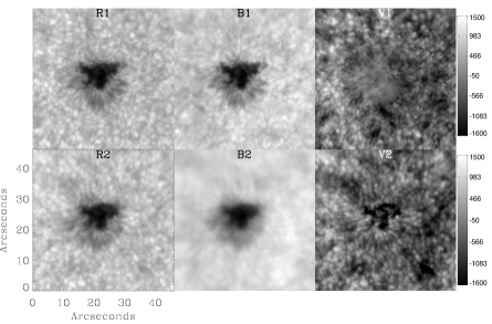
Figure 1.: Images showing the effect of variable seeing on velocity map. Top row images show a sample good red- (R1), blue-wing intensity images (B1) and the velocity map (V1) derived from these wing intensity images. Bottom row shows the same but observed during variable seeing conditions. vel˙image

An example of the effect of variable seeing is shown in Figure vel_image. The observations were obtained at the Dunn Solar Telescope (DST) in Sunspot, NM, USA using the UBF system. The images marked with R and B (R1, R2, B1, and B2) are the red- and blue-wing images whereas the images marked with V (V1 and V2) are the estimated velocities from the respective R and B. The top row images were obtained under stable seeing conditions whereas the bottom row during variable seeing conditions. The velocity map clearly shows spurious velocity signals in the umbral and penumbral regions under variable seeing conditions. This is also true with quiet solar granulation (not shown here) but not so obvious to the eye due to the high intensity-velocity correlation at these regions.

The aim of this paper is to quantitatively estimate the variable seeing-induced spurious velocity signals, through simulations and to compare them with observations. In Section S-simul, the method used to simulate the variable seeing conditions is explained and the input data used for the simulation are also explained. In Section S-results, results from the simulation using both space- and ground-based data are discussed. The comparison of the simulation results with the observed data and a summary are given in Section S-summary. We conclude with the result that there is a good correlation between seeing difference and spurious velocity signals, especially in the umbral region of the spots. Our simulation indicates that spurious velocities can be as large as 1 km s^-1 and it is alarming to note that such high values are seen in the observed data.

2 Simulations

S-simul

To simulate the effect of variable seeing on the Doppler velocities, the red- and blue-wing images, initially unaffected by the atmospheric turbulence, were convolved with point spread functions (PSFs) produced using different $r_{0}$. The PSFs were generated using the software tool Adaptive Optics Performance Evaluator (AOPE), originally developed for performing simulations on the design needs of solar adaptive optics systems [Sridharan and Bayanna (2004)].

2.1 AOPE

SS-aope A detailed description of the effect of the atmospheric turbulence on the quality of the images obtained with ground-based telescopes can be found in Roddier1981. The instantaneous wavefront perturbations induced by the atmosphere can be represented as a two-dimensional phase screen. AOPE generates such phase screens following the Kolmogorov model of turbulence, for any given value of Fried’s parameter ($r_{0}$) and derives a long-exposure PSF from them for a chosen telescope diameter and observing wavelength. AOPE also simulates the effect of the adaptive optics correction by fitting a model phase screen with finite number of Zernike polynomials (which are generally used in characterising the aberrations in optical systems) to the originally generated phase screen and subtracting the best fit model phase screen from the original phase screen. The long-exposure PSFs after adaptive optics correction are then generated from a series of residual phase screens, again for a chosen telescope diameter and wavelength. Thus, Fried’s parameter, telescope diameter, number of equivalent Zernike modes corrected by the adaptive optics system and the observing wavelength are the input parameters to be selected by the users. Long-exposure PSFs with and without a finite number of Zernike-mode correction, and ideal PSF of the telescope are the output parameters. These output parameters are characterised with the Strehl ratio, normalised Strehl resolution and the strehl width which quantify the final image quality for a given set of input parameters. In our simulations, we used this tool to obtain the ideal PSF of the telescope, and the PSFs with and without the required Zernike correction. The corrected PSF depends on all the four input parameters, whereas uncorrected PSFs do not depend on $Z$, the order of Zernike correction. The ideal PSFs depend only on telescope diameter and wavelength $\lambda$.

2.2 Input Data and Calibration

SS-data

The input data used for the simulation are obtained using the Solar Optical Telescope (SOT) on-board Hinode - a satellite dedicated for solar observations. Hinode is a joint mission between the space agencies of Japan, United States, Europe, and United Kingdom [Kosugi et al. (2007)]. Being a space-based instrument, the data obtained from SOT are free from atmospheric turbulence. The narrow-band filter imager (NFI) on SOT is used to observe wing images of magnetically insensitive ($g=0$) Fe i line ($\lambda$=5576Å ) [Tsuneta et al. (2008), Suematsu et al. (2008)]. The observations were carried out on 2007 July 14, 11:34 UT of an active region NOAA 10963. A pair of images observed at the wings ($\pm$136mÅ away from the line core) of the Fe i line 5576.09Å  are used as the input images for this simulation.

Figure 2.: Velocity versus normalised intensity difference curves estimated for the spectral lines Fe i 5434 Å (wing points at $\pm$ 60 mÅ ; represented by asterisks) and Fe i 5576 Å (wing points at $\pm$ 136 mÅ ; represented by pluses). Solid and dashed lines are straight line fits to the respective curves. ubfcal

The input data for the simulation of ground-based images are obtained using UBF observation of a sunspot carried out at the Dunn Solar Telescope (DST), NSO, NM, USA, on 2005 December 28. The calibration constant $C$ (cf. Equation (1)), required for deriving the velocity from the observed normalised intensity difference $\delta I$ ( = $\frac{I_{\rm r}-I_{\rm b}}{I_{\rm r}+I_{\rm b}}$), is estimated using the spectral profile from the Liège atlas. First, the atlas profile of the observed line is convolved with a Gaussian filter profile of passband specific to the instrument used. In this paper, data from the NFI on-board Hinode as well as from the UBF at the Dunn Solar Telescope are used. The passband is estimated to be 70 mÅ in the case of NFI and 142 mÅ for the UBF. The Doppler shift of the spectral line $\Delta\lambda$ for a defined velocity $v$ is calculated by using $\frac{\Delta\lambda}{\lambda}=\frac{v}{c}$ where $c$ is the speed of light. The convolved spectral line is then shifted by an amount of $\Delta\lambda$ and the normalised intensity difference is calculated. This is repeated for a range of velocities. Figure ubfcal shows the relation between $\Delta v$ and $\delta I$ for both 5576 Å (plus) and 5434 Å (asterisks) spectral lines. The linear part of the curve is fitted with a straight line (solid and dashed lines respectively) and 1/slope provides the calibration constant value $C$. For large velocity values, either the line core or the continuum will cross one of the chosen wing wavelengths and hence the $\delta I$ curve will deviate from the straight line. This sets the limit for the velocity range that can be measured using this method. The velocity range and the slope value (or calibration constant $C$) depends on the spectral line and the chosen wing pair. This is clearly reflected in Figure ubfcal in which the dynamic range achieved for Fe i 5576 Å  is smaller compared to that of Fe i 5434 Å .

2.3 Procedure

SS-procedure The simulation is carried out for a telescope diameter of 50 cm (commensurate with Hinode) and for different Fried’s parameter values (starting from $r_{0}$ = 4 cm to 15 cm). In typical ground-based solar observations, Fried’s parameter of 4 cm or below is considered as bad seeing and an $r_{0}$ of 12 cm or above is considered as an excellent seeing condition. For each $r_{0}$ values, PSFs with and without Zernike corrections (of a particular order) are generated. For the simulation, Zernike order is varied from 11 to 55 depicting different amount of AO corrections. The PSFs generated are then convolved with the input image to generate different observational conditions. In order to simulate the variable seeing effects, the blue- and red-wing images are convolved with different PSFs generated using different $r_{0}$ as well as different Zernike correction.

The velocities are derived using Equation (eq1) for different simulated conditions. The generated velocity images are used to quantify the effect of variable seeing conditions. The umbra, penumbra, and quiet Sun regions are analysed separately in order to quantify the effects in these different regions.

For quantifying such variable seeing conditions between blue- and red-wing images, we define the normalised seeing difference $(\delta r_{0})$ by,

$$\delta r_{0}=\frac{r_{\rm 0R}-r_{\rm 0B}}{r_{\rm 0R}+r_{\rm 0B}},\ilabel{eq2}$$ (2)

where $r_{\rm 0R}$ and $r_{\rm 0B}$ are the seeing during the red- and blue-wing observations respectively.

3 Results

S-results

The top row of Figure hinode_fig2 shows a pair of red- and blue-wing images and the velocity image used in our simulation. The velocity image in the top row shows the typical granular flows in the quiet region, Evershed flows in the penumbral region and uniform or zero flows in the umbral region. The grey scale used for the velocity images are also marked as a colour bar on the right side of the velocity figures. The bottom row shows the best case scenario when the seeing is good, like with the case of $r_{0}$ = 15 cm and high order AO correction ($Z$ = 66). The estimated velocity image looks similar to the original. The middle row shows a seeing-affected blue-wing image simulated for $r_{0}$ = 4 cm and without AO correction (the worst case scenario), the original red-wing image (convolved with ideal PSF), and the resulting velocity image. Note the change in the velocity values and the appearance of velocity structures in the umbra. These small-scale structures resemble umbral dots in the intensity image and hence are considered as cross-talk from intensity. This clearly shows the effect of the seeing difference inducing spurious velocity structures as well as modifying the velocity amplitudes. These effects are most notable in the umbral region.

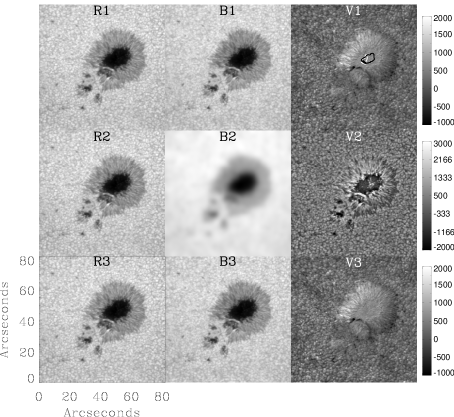
Figure 3.: Hinode SOT-NFI images showing the effect of seeing difference on velocity. This figure is similar to Figure vel_image except that it is simulated. The top row shows the original red- (R1), blue-wing (B1) images and the corresponding velocity map (V1). The middle row shows the original red- (R2), convolved blue-wing (B2) images and the corresponding velocity (V2). B2 is created by convolving original blue-wing image with a PSF of $r_{0}$ = 4 cm and without AO correction. In the bottom row, B3 is created by convolving original blue-wing image with the PSF of $r_{0}$ = 15 cm and $Z$=66. The colour bars on the right-hand side shows the grey scale range for the corresponding velocity images. Dark and white contours in V1 are the regions selected for measuring $\sigma$ and $\mu$, respectively.

hinode_fig2

In order to quantitatively study the effect on the mean velocity ($\mu$), a core umbral region with minimal intensity structures (like umbral dots) is selected manually. This region is shown as a white contour in V1 of Figure hinode_fig2. The spurious velocity structures (as seen in V2 of Figure hinode_fig2) are quantified using the standard deviation of the velocity of an umbral region which includes the umbral structures (like umbral dots) and this is shown as a dark contour in V1 of Figure hinode_fig2. The two parameters ($\mu$ and $\sigma$) are plotted with normalised seeing difference (cf. Equation (eq2)) in Figure hinode1. The seeing difference is simulated by convolving one of the wing images (either red or blue) with a PSF of a fixed Fried’s parameter (called base seeing in this paper), and the other wing is convolved with PSFs corresponding to variable Fried’s parameter ($r_{0}$ = 4 to 15 cm). This is repeated by varying the base seeing values from 4 to 15 cm. The normalised seeing difference is calculated as per Equation (eq2), and the mean velocity is calculated at the selected core umbral region. The same is also repeated with AO corrected PSFs, with Zernike correction order varying from $Z$=11 to $Z$=55.

In Figure hinode1, the normalised seeing difference versus umbral core mean velocity is plotted on the left column. The top plot is the case without AO correction, the middle plot is with a Zernike correction of $Z$=11 and the bottom one is for $Z$=55. All the plots have three types of symbols. Squares are for base seeing, where either $r_{\rm 0R}$ or $r_{\rm 0B}$ is equal to 15 cm and the other varying from 15 to 4 cm. In other words, one of the wing images is affected by the best seeing condition and the other varies from best to worst. Similarly, asterisks are for a base seeing of 4 cm and pluses are for 9 cm. Each curve has two parts, separated by zero $\delta r_{0}$, and positive abscissa ( positive $\delta r_{0}$) means $r_{\rm 0R}~{}>~{}r_{\rm 0B}$. All the symbols are just connected by lines of different line types. As seen in the right column of Figure hinode1, the standard deviation ($\sigma$) varies with seeing difference and hence cannot be used as an error estimate for $\mu$. The standard deviation of the velocity estimated in the selected umbral region of the original velocity image is used as the error in the velocity estimates for all simulated conditions.

All the three plots show that spurious velocity values increase with normalised seeing difference. For a particular normalised seeing difference value, there is a range of velocity values depending on the base seeing condition. A poor base seeing, or the dashed line in the plot (connecting asterisks, where either $r_{\rm 0R}$ or $r_{\rm 0B}$ is equal to 4 cm), represents the maximum limit, and a good base seeing, solid line (connecting squares, where either $r_{\rm 0R}$ or $r_{\rm 0B}$ is equal to 15 cm) is the minimum limit of these induced velocities. Notice that the range comes to almost zero at zero normalised seeing difference, irrespective of the difference in the base seeing. As AO corrections are applied (middle and bottom plots), both the maximum and minimum limit of the induced velocity decreases.

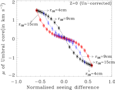
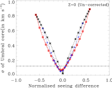
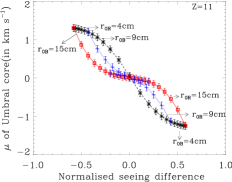
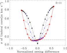
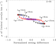
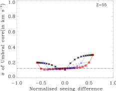
Figure 4.: Effect of seeing difference on mean velocity (left column) and on velocity structures (right column) in the umbral region. The top row is the case without AO correction, the middle one with a Zernike correction of 11 and the bottom one with a correction of 55. In all the plots, squares represent the best seeing case when $r_{\rm 0R}$ or $r_{\rm 0B}$ = 15 cm and the solid line connects the symbols, pluses are for $r_{\rm 0R}$ or $r_{\rm 0B}$ = 9 cm, asterisks are for $r_{\rm 0R}$ or $r_{\rm 0B}$ = 0 cm and the dotted lines and dashed lines connect the symbols, respectively. hinode1

In the right column of Figure hinode1, the standard deviation of the selected umbral area is plotted with normalised seeing difference. The top plot is without AO correction, the middle one with a Zernike correction of $Z$=11 and the bottom one with $Z$=55. The horizontal line is the value of $\sigma$ of the original velocity image. It is clear from the curves that the seeing difference introduces spurious velocity structures in the selected umbral region, and AO with higher order correction helps in minimising these induced spurious velocity structures. When both wing images are affected by similar bad seeing, the fine scale intensity structures are smeared in both. Hence the intrinsic velocity contrast of these structures is reduced representing the points below the horizontal line.

A similar study is carried out for the penumbral regions. However, due to the presence of Evershed flows, the mean velocity ($\mu$) was calculated separately for positive and negative velocities (flows away from and towards the observer). The standard deviation of the selected penumbral area is a measure of penumbral structures. These two parameters are plotted in Figure hinode2 for different Zernike corrections. It is clear from the figure that $\mu$ (left column) in a penumbra increases very little (200-300 m s^-1) with normalised seeing difference, whereas $\sigma$ (right column) increases significantly. Similar to the umbral structures, with higher order AO correction $\sigma$ falls off to original and also $\sigma$ does not fall to zero due to the existence of penumbral velocity structures in the input image. In the case of the penumbra, $\sigma$ of the input image cannot be taken as the error in the velocity estimate due to the presence of Evershed flow velocity structures, and hence the error bars are not displayed. Horizontal lines show the value of $\sigma$ estimated from the initial velocity image.

The quiet sun-study showed a similar behaviour (with weaker amplitudes) like the penumbra and hence is not discussed in this paper.

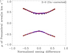
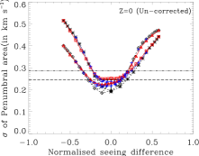
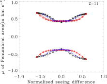
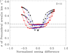
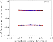
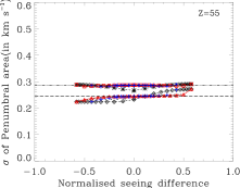
Figure 5.: Similar to Figure hinode1 but for the penumbral region. The mean velocity is calculated separately for positive (towards the observer) and negative (away from the observer) cases. Squares (positive side) and triangles (negative side) represent the best base seeing condition ($r_{\rm 0R}$ or $r_{\rm 0B}$ = 15 cm). Similarly, asterisks (positive side) and diamonds (negative side) represent the bad base seeing condition (4 cm), and pluses represent the medium seeing condition (9 cm). Lines are just a connection of data points. hinode2

3.1 Ground-Based Observations

SS-ground

A similar study is carried out with images obtained from ground-based observation. The seeing was variable at the time of observation. About 3 s was required to tune UBF from one wing to the other wing. Due to the variable seeing condition, there were many wing-pair images affected by the seeing difference in the observed data (one such an example is shown in Figure vel_image). From the observed data, a pair of best images were chosen as input for the simulations. Differential seeing was simulated as explained in the previous section.

The curves of $\mu$ and $\sigma$ are very similar to the curves seen in Figure hinode1, and hence they are not reproduced here in this paper. The only notable difference was in the $\sigma$ curves and that can be attributed to the difference in the umbral structures for these two different sunspot regions.

4 Summary and Discussions

S-summary

In the velocity measurements from the ground using narrow-band filters, there is always a chance of systematic error in velocity estimates due to the seeing difference. If seeing changes within the time of wavelength tuning from one wing to the other, it will create spurious velocity values. We simulated such seeing difference conditions using the AOPE code, and we studied the induced velocity values in different areas of a solar active region (like umbra, penumbra, and quiet sun). It is concluded that the seeing difference affects the velocity estimates more in the umbra than in the penumbral region of the sunspot. It is also seen that the effect is minimal in the quiet sun. Under worst normalised seeing difference conditions, where one wing image is obtained under a good seeing condition ($r_{0}$ = 15 cm) and the other during worst condition ($r_{0}$ = 4 cm; $\delta r_{0}$=0.58), the induced velocity is as high as 1 km s^-1. Such a large variation in seeing may not occur often in real cases, but our sample observations (e.g. Figure vel_image) using the UBF at the DST have shown velocities up to 600 m s^-1. It is also clear that these induced velocity structures are due to cross-talk from intensity. A correlation analysis carried out between intensity and velocity shows a correlation coefficients up to 50% in the worst case scenario. These simulations also show that adaptive optics corrections can significantly reduce such induced velocities, and velocity structures.

Figure 6.: Scatter plot between normalised seeing difference and normalised contrast difference from the simulations using NSO data as the input.dcontra

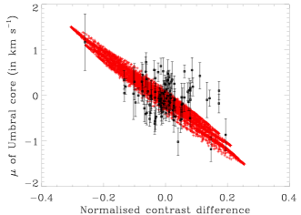
Figure 7.: Graph showing umbral core velocity with normalised contrast difference. The filled squares are from the observation and red pluses are from the simulation. The error bars on the observed points are three times the standard deviation of the umbral core velocity distribution.final˙plot

We used UBF observations carried out during variable seeing conditions to compare with the simulations. However, in order to compare with the real observations, contrast values are used as a measure of seeing, since there were no simultaneous measurements of Fried’s parameter. The contrast at the umbra-penumbra border was used as a measure of seeing rather than the quiet-sun contrast. This is because the lock point of AO was in the umbra-penumbra border. The AO correction away from the lock point was really variable due to the variable seeing condition and hence contrast obtained at these areas will not represent the seeing changes alone in the umbra. We have also taken care to choose the region which has a minimum velocity throughout the time sequence of roughly 2 hours, as velocity can also change the intensity contrast. We define contrast as the standard deviation of the selected region in the intensity image. The normalised contrast difference is defined as the ratio between the difference and total of the blue- and red-wing contrasts and hence is a proxy for the normalised seeing difference value. Figure dcontra shows the relation between normalised seeing difference and normalised contrast difference from simulations with NSO data as the input. It is clear from the plot that the spread in the curve will cause a degeneracy in the normalised contrast difference values for a particular normalised seeing difference. Also, the zero normalised contrast difference does not fall on the zero normalised seeing difference and vice versa. This shift can be associated to the seeing difference in the input wing images and to the convective blue-shift.

Figure final_plot shows the scatter plot between the normalised contrast difference versus $\mu$ at the core umbra estimated for the NSO data. Squares are from observation and pluses are from simulation. The simulation was extended to include all combinations of seeing values varying from $r_{0}$ = 4 to 15 cm and a Zernike correction from $Z$ = 11 to 77 to mimic a real observation. The error bar of the original data points are three times the standard deviation ($\sigma$) of the velocity distribution in the selected umbral core region. The value of this $\sigma$ will be a combination of the actual error in the velocity estimation and the standard deviation due to the induced structures because of the seeing difference.

In general most of the data points (70%) fall within the simulated velocity distribution. However, there are points well away from the simulated curve which may be due to (1) the observed data being a time sequence spanning approximately 2 hours, and hence any evolution can change both the velocity value and the contrast, (2) simulation assuming noiseless PSF after perfect AO correction whereas in a real situation it will not be.

We conclude the folloeing. (1) A seeing difference introduces spurious velocity signals which are large in the umbra compared to the penumbra and the quiet sun due to the low intrinsic velocities inside the umbra. (2) The spurious velocity also depends on the base seeing condition. If the general seeing conditions are very bad, then even a small seeing difference can cause large spurious velocity. (3) The simulations have given a range of spurious velocity, for a particular seeing difference in very bad base seeing condition ($r_{0}$= 4 cm) and for very good base seeing condition ($r_{0}$ = 15 cm). For a normalised seeing difference condition of 0.5 this spurious velocity can range from 600 m s^-1 ( good base seeing) to 1200 m s^-1 (bad base seeing). A normalised seeing difference of 0.5 in the umbra occurs when the ratio of Fried’s parameter between the red- and blue-wing images is larger than 3. A normalised seeing difference of 0.5 corresponds to a normalised contrast difference of approximately 0.2 and such values are seen in the observed data. (4) With higher order AO corrections, the spurious velocities are reduced by a factor greater than 4 for a normalised seeing difference of 0.5 or less for a perfect AO system.

We wish to caution the reader that this simulation is just to approximate the range of errors induced due to a seeing difference in velocity measurements based on a narrow-band filter. An error in the range of 1 km s^-1 is important in areas like the umbra and penumbra at the photospheric level. These results cannot be used to remove the spurious velocities from the seeing-affected observed images. At the same time, we cannot ignore all seeing-affected data, especially in the case of observation of transient phenomena like penumbral formation or a flare. In real observational situations, PSFs can vary even when $r_{0}$ remains constant (especially for exposures not long enough to average out the seeing fluctuations). In our simulation, it is assumed that the changes in PSFs are only due to changes in $r_{0}$. If PSFs can be estimated using the AO data simultaneously along with the Doppler measurements, then the variable seeing effects could be minimised by using deconvolution techniques [Rimmele and Marino (2006)]. In the future, new methods and technologies may also be developed to observe the blue- and red-wing images simultaneously to avoid such effects.

Hinode is a Japanese mission developed and launched by ISAS/JAXA, collaborating with NAOJ as a domestic partner, NASA and STFC (UK) as international partners. Scientific operation of the Hinode mission is conducted by the Hinode science team organised at ISAS/JAXA. This team mainly consists of scientists from institutes in the partner countries. Support for the post-launch operation is provided by JAXA and NAOJ (Japan), STFC (U.K.), NASA, ESA, and NSC (Norway).

References

- Beckers et al. (1975) Beckers, J.M., Dickson, L., Joyce, R.S.: 1975, AFCRL Report No. AFCRL-TR-75-0090, Air Force Cambridge Research Laboratory, Massachusetts.
- Bharti, Jain, and Jaaffrey (2007) Bharti, L., Jain, R., Jaaffrey, S.N.A.: 2007, ApJ 665, 79.
- Cavallini (2006) Cavallini, F.: 2006, Sol. Phys. 236, 415.
- Kosugi et al. (2007) Kosugi, T., Matsuzaki, K., Sakao, T., Shimizu, T., Sone, Y., Tachikawa, S., et al.: 2007, Sol. Phys. 243, 3.
- Rajaguru et al. (2007) Rajaguru, S.P., Sankarasubramanian, K., Wachter, R., Scherrer, P.H.: 2007, ApJ 654, 175.
- Rimmele (2008) Rimmele, T.: 2008, ApJ 672, 684.
- Rimmele and Marino (2006) Rimmele, T., Marino, J.: 2006, ApJ 646, 593.
- Rimmele (1995) Rimmele, T.: 1995, A&A 298, 260.
- Rimmele et al. (2006) Rimmele, T., Roche, J.: 2006, ATST Project Documentation TN-0073, National Solar Observatory.
- Rimmele (2004a) Rimmele, T.: 2004, ApJ 604, 906.
- Rimmele (2004b) Rimmele, T.: 2004, In: Bonaccini Calia, D., Ellerbroek, B.L., Ragazzoni, R. (eds.), Advancements in Adaptive Optics, Proc. SPIE 5490, 34.
- Roddier (1981) Roddier, F.: 1981, Prog. Optics 19, 281.
- Sankarasubramanian and Hagenaar (2007) Sankarasubramanian, K., Hagenaar, H.: 2007, Bull. Astron. Soc. India 35, 427.
- Sankarasubramanian and Rimmele (2003) Sankarasubramanian, K., Rimmele, T.: 2003, ApJ 598, 689.
- Scharmer et al. (2002) Scharmer, G.B., Gudiksen, B.V., Kiselman, D., Löfdahl, M.G., Rouppe van der Voort, L.H.M.: 2002, Nature 420, 151.
- Schüssler and Vögler (2006) Schüssler, M., Vögler, A.: 2006, ApJ 641, 73.
- Sridharan and Bayanna (2004) Sridharan, R., Bayanna, A.R.: 2004, In: Fineschi, S., Gummin, M.A., (eds.), Telescopes and Instrumentation for Solar Astrophysics, Proc. SPIE 5171, 219.
- Stix (2002) Stix, M.: 2002, The Sun, Springer Publications., 106.
- Suematsu et al. (2008) Suematsu, Y., Tsuneta, S., Ichimoto, K., Shimizu, T., Otsubo, M., Katsukawa, Y., et al.: 2008, Sol. Phys. 249, 197.
- Tsuneta et al. (2008) Tsuneta, S., Ichimoto, K., Katsukawa, Y., Nagata, S., Otsubo, M., Shimizu, T., et al.: 2008, Sol. Phys. 249, 167.
- Wachter, Schou, and Sankarasubramanian (2006) Wachter, R., Schou, J., Sankarasubramanian, K.: 2006, ApJ 648, 1256.