Deducing spectroscopic factors from wave-function asymptotics

Abstract

In a coupled-channel model, we explore the effects of the coupling between configurations on the radial behavior of the wave function and in particular on the spectroscopic factor (SF) and the asymptotic normalisation coefficient (ANC). We evaluate the extraction of a SF from the ratio of the ANC of the coupled-channel model and that of a single-particle approximation of the wave function. We perform this study within a core$+n$ collective model, which includes two states of the core that connect by a rotational coupling. To get additional insights, we also use a simplified model that takes a delta function for the coupling potential. Calculations are performed for ¹¹Be. Fair agreement is obtained between the SF inferred from the single-particle approximation and the one obtained within the coupled-channel models. Significant discrepancies are observed only for large coupling strength and/or large admixture, i.e. small SF. This suggests that reliable SFs can be deduced from the wave-function asymptotics when the structure is dominated by one configuration, i.e. for large SF.

I Introduction

Historically, direct reactions have been an important source of information on nuclear structure. The development of radioactive-ion beams has rekindled the interest in those reactions by providing a unique way to study nuclei far from stability Fulton (2010). Through direct reactions, it is indeed possible, with an appropriate reaction model, to extract quantitative information on the structure of nuclei bound for only milliseconds Roussel-Chomaz (2010). For example, the orbital configuration of the valence nucleons in a number of neutron-rich nuclei has been determined through transfer Thomas et al. (2007), knockout Hansen and Tostevin (2003) and breakup Nakamura et al. (1999) reactions.

The abrupt nature of direct reactions leads to limited structural changes in the involved nuclei. Therefore, the cross sections for those reactions can be expressed in terms of overlap functions, which, strictly, involve overlap integrals of the full wave functions for the initial and final states of the nuclei Thompson and Nunes (2009). Information about overlap functions can be inferred from direct reactions. In particular, the square of its norm, called spectroscopic factor (SF), is supposed to be obtained from a comparison between theory and experiment. Some controversy exists about the use of SFs when discussing nuclear structure Furnstahl and Hammer (2002); Furnstahl and Schwenk (2010). Nevertheless, SFs are attractive in that they give an insight into the complexity of the nuclear states involved in the reaction. Moreover, they can be compared to results of electron inelastic scattering and of shell-model calculations. Alternatively, it has been suggested that, since direct reactions are mostly peripheral, they probe only the tail of the overlap function Mukhamedzhanov and Nunes (2005); Capel and Nunes (2007). Accordingly, only the asymptotic normalization coefficient (ANC) of the overlap function should be extracted from data analysis.

Currently there is no fully microscopic basis for calculating overlap functions for nuclei with mass $A>10$, let alone a reaction model that includes these microscopic overlap functions. Reaction data are usually analyzed within models where nucleons are grouped into few clusters, and in which overlap functions are substituted by wave functions obtained by solving a Schrödinger equation in which the interactions between the clusters are simulated by local potentials. As the primary application of this work is the study of nuclear structure far from stability, we consider the case of two-cluster systems, such as one-neutron halo nuclei, in which a neutron is loosely bound to the core of the nucleus. In that case, the overlap function is approximated by a single-particle wave function, which describes the valence neutron evolving in a mean-field potential representing its interaction with the core. The cross section obtained with this single-particle approximation of the overlap function is renormalized to match experimental data and, from that renormalization, a SF or an ANC is deduced. In this work, we examine the validity of these assumptions by addressing the following questions: First, how accurately can one substitute the exact overlap function by a single-particle wave function? Second, if only the ANC can be extracted from measurements, can it be reliably related to the SF?

Within a fully microscopic description of the nuclei, overlap functions satisfy a set of strongly coupled equations. Formally, this set can always be reduced to one equation for the single function of interest, evolving under the influence of an effective single-particle Hamiltonian. However, due to strong couplings between the different channels, that Hamiltonian is going to be highly nonlocal, in terms of its dependence on both position and energy. For instance, it will describe absorption of the probability flux from one channel into another channel. This transfered probability flux may be absorbed from one side of the nucleus and returned to the other side of the nucleus. Obviously, this involves a significant spatial nonlocality, up to the size of the nucleus. The associated energy dependence of the effective Hamiltonian may be tied to the time delay in returning the flux to the original channel. Needless to say that such type of effects cannot be properly accounted for in terms of a simple local potential. By contrast, coupling effects with exchange of probability flux between channels may be adequately simulated at a semiquantitative level in collective models.

In this work, we consider the rotational-coupling model developed by Nunes et al. Nunes et al. (1996); Thompson et al. (2004). In that model, the core of the nucleus is described as a deformed rotor, which can be in various excited states. This leads to a set of coupled equations for the core-nucleon wave functions similar to those obtained within microscopic models. The rotational model is applied to ¹¹Be, the archetypal one-neutron halo nucleus. This nucleus is described as a neutron loosely bound to a ¹⁰Be core which can be in both its $0^{+}$ ground state and $2^{+}$ excited state Nunes et al. (1996). Note that similar models have been developed by other groups, see e.g. Refs. Esbensen et al. (1995); Vinh Mau (1995).

In order to assess the validity of the single-particle approximation, and to understand the influence of the couplings upon an overlap function, its SF, and ANC, we carry out cross-comparisons within theory. We analyze the more realistic rotational model in terms of the single-particle approximation. In particular we compute the ANCs within the rotational model and the single-particle approximation and we deduce a SF from their ratio. Confronting the deduced SF to that directly obtained within the rotational model, we can infer the reliability of the extraction of SFs from ANCs. This method could prove very valuable if ANCs can be efficiently measured from direct reactions, like transfer Mukhamedzhanov and Nunes (2005) or breakup Capel and Nunes (2007). Note that besides the accuracy of the method, the extraction of SFs from ANCs is subject to other uncertainties. In particular, the geometry of the core-neutron potential is not known a priori. In this work, we focus on the validity of the method and disregard this latter uncertainty Mukhamedzhanov and Nunes (2005); Pang et al. (2007); Mukhamedzhanov et al. (2008). Throughout our analysis, we always use the same potential geometry within both the rotational model and the corresponding single-particle approximation.

Besides the aforementioned rotational model Nunes et al. (1996); Thompson et al. (2004), we also employ a simplified schematic model with two overlap functions generated with square-well potentials and coupled by a delta function. This simplified model may be largely solved analytically, which enables us to interpret qualitatively the results of the rotational model.

An important issue not treated in the present work is the effect of short-range correlations, which can contribute to the lowering of SF. Those correlations are often the focus of investigations in many-body theory of nuclear matter Dickhoff and Barbieri (2004). They generally affect the overlap function within the nuclear volume, just as do the couplings to collective states. Hence, although not exactly included here, short-range correlations will be qualitatively simulated within the rotational model.

Direct reactions are a useful tool to study nuclear structure far from stability. However, many uncertainties remain in the analysis of measurements. While significant advances have been made recently on the side of reaction theory Summers et al. (2006a, b); Matsumoto et al. (2006); Rodríguez-Gallardo et al. (2008); Baye et al. (2009), the models employed in the analysis remain fairly schematic relative to the full many-body problem. On the structure side, the attention of microscopic models has been primarily directed at the treatment of short-range correlations. Traditionally, little attention was paid to the asymptotic part of the wave functions Pieper and Wiringa (2001); Forssén et al. (2008), which is essential in the analysis of direct reactions. More recently, there have been works focusing on the asymptotic behavior Quaglioni and Navrátil (2009); Timofeyuk (2010); Brida and Nunes (2010). However, the task of establishing this behavior may become very complicated for loosely-bound nuclei, and even more if multiple-channel configurations are involved. For these and other reasons, the single-particle model is likely to remain a work horse in data analysis in the near future. Therefore, assessing uncertainties associated with that model is important.

In the next section we provide the necessary theoretical background for this study. We first introduce the notion of overlap functions and their couplings. We then present the various models used in this work: the single-particle model, the rotational model, and the schematic delta-coupling model. In Sec. III, we provide quantitative results. First, we study the realistic conditions for the case of ¹¹Be. Second, we explore the limits of the parameter space in the effort to draw general conclusions. Finally, we investigate these results within the more schematic delta-coupling model. Our work is summarized in Sec. IV.

II Theoretical considerations

II.1 Overlap function, SF, and ANC

Within direct-reaction theory, the cross sections for transfer, break-up, or knockout are usually expressed in terms of overlap functions Thompson and Nunes (2009). The reaction is indeed expected to reveal the dominant configuration within the projectile structure, such as $A\rightarrow B+n$. Here and in the following, we consider a nucleus $A$ that exhibits a strong two-cluster structure: a valence neutron $n$ bound to a core $B$. To simplify matters, the symbols $A$ and $B$ will also stand for the mass numbers, i.e. $B=A-1$.

As an introductory step, we derive the equations satisfied by the overlap wave function within a general many-body formalism. We will specifically refrain from discussing the issues of spin, some antisymmetrization effects and center-of-mass corrections. With the exception of antisymmetrization, which cannot be considered exactly in a collective model, these will be accounted for in the practical calculations.

Formally, the microscopic Hamiltonian describing the motion of the nucleons of nucleus $A$ reads:

$$H_{A}=\sum_{i=1}^{A}t_{i}+\sum_{j>i=1}^{A}v_{ij}\,,$$ (1)

where $t_{i}$ is the kinetic-energy operator for nucleon $i$ and $v_{ij}$ describes the interaction between nucleons $i$ and $j$. For simplicity, we do not mention three-body interactions. The states $\nu_{A}$ of $A$ are the eigenstates of $H_{A}$,

$$E_{\nu_{A}}^{A}\,\Psi_{\nu_{A}}(\mbox{\boldmath$r$}_{1},\ldots,\mbox{\boldmath$r$}_{A})=H_{A}\,\Psi_{\nu_{A}}(\mbox{\boldmath$r$}_{1},\ldots,\mbox{\boldmath$r$}_{A})\,,$$ (2)

where $\{\mbox{\boldmath$r$}_{i}\}$ are the coordinates of the nucleons of $A$. Similarly, an $(A-1)$-body Hamiltonian, with eigenstates $\Phi_{\nu_{B}}$ of energy $E_{\nu_{B}}^{B}$, can be defined for the core $B$. As mentioned earlier, the states of $A$ may present a strong $B$-$n$ cluster structure. In that case, it is worthwhile to describe the relative motion between the core in its state $\nu_{B}$ and the valence neutron in terms of the overlap function $\psi_{\nu_{A}\,\nu_{B}}$, which is nothing but the projection of $\Psi_{\nu_{A}}$ onto the wave function describing the core state $\Phi_{\nu_{B}}$,

$$\psi_{\nu_{A}\,\nu_{B}}(\mbox{\boldmath$r$})= \int d\mbox{\boldmath$r$}_{1}\cdots d\mbox{\boldmath$r$}_{A-1}\,\Phi_{\nu_{B}}^{*}(\mbox{\boldmath$r$}_{1},\ldots,\mbox{\boldmath$r$}_{A-1})$$ (3)

$$\times\Psi_{\nu_{A}}(\mbox{\boldmath$r$}_{1},\ldots,\mbox{\boldmath$r$}_{A-1},\mbox{\boldmath$r$})\,,$$

where $r$ is the coordinate of the valence neutron relative to the core.

The spectroscopic factor is defined as the square of the norm of the overlap function:

$$S_{\nu_{A}\,\nu_{B}}=\int d\mbox{\boldmath$r$}\,|\psi_{\nu_{A}\,\nu_{B}}(\mbox{\boldmath$r$})|^{2}.$$ (4)

This SF represents the probability that, within the state $\nu_{A}$ of $A$, the neutron may be found in a combination with the core $B$ in state $\nu_{B}$. The SFs add up to unity over all the states of $B$, including those in the continuum,

$$\sum_{\nu_{B}}S_{\nu_{A}\,\nu_{B}}=1,$$ (5)

since that sum represents the square of the norm of $\Psi_{\nu_{A}}$.

To obtain the formal equations satisfied by the overlap function, we project both sides of Eq. (2) onto $\Phi_{\nu_{B}}$. Taking account of Eq. (3), we obtain

$$E_{\nu_{A}}^{A}\, \psi_{\nu_{A}\,\nu_{B}}=\langle\Phi_{\nu_{B}}|H_{A}|\Psi_{\nu_{A}}\rangle$$

$$=(E_{\nu_{B}}^{B}+t_{\mbox{\boldmath$r$}})\,\psi_{\nu_{A}\,\nu_{B}}+\sum_{\mu_{B}}V_{\nu_{B}\,\mu_{B}}\,\psi_{\nu_{A}\,\mu_{B}},$$ (6)

where $t_{\mbox{\boldmath$r$}}$ is the $B$-$n$ kinetic-energy operator and

$$V_{\nu_{B}\,\mu_{B}}=\langle\Phi_{\nu_{B}}|\sum_{i=1}^{B}v_{in}|\Phi_{\mu_{B}}\rangle$$ (7)

are potential terms that couple different possible configurations $\nu_{A}\,\nu_{B}$ within $\Psi_{\nu_{A}}$. Let us now define the energy of the state $\nu_{A}$ relative to the $B$-$n$ threshold (i.e. the negative of the separation energy) by

$$\varepsilon_{\nu_{A}}^{Bn}=E_{\nu_{A}}^{A}-E_{0}^{B}\,,$$ (8)

and the core excitation energy by

$$\epsilon_{\nu_{B}}=E_{\nu_{B}}^{B}-E_{0}^{B}\,.$$ (9)

In Eqs. (8) and (9), $E_{0}^{B}$ is the ground-state energy of $B$, hence $\varepsilon_{\nu_{A}}^{Bn}<0$ for particle stable $A$ and $\epsilon_{\nu_{B}}\geq 0$. The set of equations (6) can now be rewritten into the form

$$(\varepsilon_{\nu_{A}}^{Bn}-\epsilon_{\nu_{B}})\,\psi_{\nu_{A}\,\nu_{B}} =(t_{\mbox{\boldmath$r$}}+V_{\nu_{B}\,\nu_{B}})\,\psi_{\nu_{A}\,\nu_{B}}$$

$$\hskip 10.00002pt+\sum_{\mu_{B}\neq\nu_{B}}V_{\nu_{B}\,\mu_{B}}\,\psi_{\nu_{A}\,\mu_{B}}\,.$$ (10)

The picture behind this set of equations is that of a neutron moving around $B$, which can be in its various states. The possible quantum numbers for the $B$-$n$ relative motion in each configuration $\nu_{A}\,\nu_{B}$ are determined by conservation laws and by the quantum numbers of the states $\nu_{A}$ and $\nu_{B}$. In particular, the orbital angular momentum $l$ of the $B$-$n$ relative motion is determined by parity conservation and angular-momentum couplings.

The diagonal potential element $V_{\nu_{B}\,\nu_{B}}$ in Eq. (10) represents the single-particle potential for $n$ being in the field of $B$ in its state $\nu_{B}$. The motion of $n$ is modified by the presence of other channels $\nu_{A}\,\mu_{B}$, which couple to $\nu_{A}\,\nu_{B}$ through the non-diagonal potential elements $V_{\nu_{B}\,\mu_{B}}$. In passing, we may note that, since the internucleon interactions $v_{ij}$ are at most weakly nonlocal, both the single-particle and the coupling potentials (7) will be at most weakly nonlocal in $r$. In addition, this weak nonlocality, combined with the short range of nuclear interaction, will lead to a form factor for the nuclear contribution to $V_{\nu_{B}\,\nu_{B}}$ that approximates the shape of the density of $B$. Outside the volume of $B$, the nuclear contributions to the potentials get suppressed and the wave equations simplify. For a $B$-$n$ system, i.e. in absence of Coulomb, the radial part of the overlap function of a configuration with orbital angular momentum $l$ exhibits the asymptotic behavior

$$\psi_{\nu_{A}\,\nu_{B}}(r)\mathop{\longrightarrow}\limits_{{r}\rightarrow{\infty}}C_{\nu_{A}\,\nu_{B}}\,i\,\kappa_{\nu_{A}\,\nu_{B}}\,h_{l}^{(1)}(i\,\kappa_{\nu_{A}\,\nu_{B}}r)\,,$$ (11)

where $\hbar\,\kappa_{\nu_{A}\nu_{B}}=\sqrt{2\mu_{Bn}|\,\varepsilon_{\nu_{A}}^{Bn}-\epsilon_{\nu_{B}}|}$, with $\mu_{Bn}$ the $B$-$n$ reduced mass, and $h_{l}^{(1)}$ is a spherical Bessel function of the third kind Abramowitz and Stegun (1970). The normalization constant $C_{\nu_{A}\,\nu_{B}}$ appearing in Eq. (11) is the asymptotic normalization coefficient. The function $h_{l}^{(1)}$ accounts for the effects of the centrifugal barrier and behaves as $\exp(-\kappa_{\nu_{A}\,\nu_{B}}r)/\kappa_{\nu_{A}\,\nu_{B}}r$ for $\kappa_{\nu_{A}\,\nu_{B}}r\gg l$. Hence, of all the different overlap functions, the one corresponding to the ground state of $B$ (i.e. with $\epsilon_{\nu_{B}}=0$) dominates the asymptotic behavior of $\psi_{\nu_{A}\,\nu_{B}}$, whereas the overlap functions corresponding to high-lying states of the core barely stick out of the volume of $B$. In the presence of couplings, any channel that satisfies the conservation laws could, in principle, contribute to the spectroscopic factor. However, in the case of loosely-bound systems, much of the wave function is expected to be outside the volume of $B$. The dominance of the $B$ ground-state channel in the asymptotic region suggests that this channel also dominates the contributions to the SF.

Due to the couplings, the shape of the overlap function $\psi_{\nu_{A}\,\nu_{B}}$ differs from the solution of a single-particle Schrödinger equation in which the nuclear $B$-$n$ interaction is simulated by a local potential tied to the density of $B$. This influence of the couplings upon the shape of the overlap function, and in particular on the connection between SF and ANC, is the focus of the present work. As mentioned in the introduction, we do not solve the full many-body problem (2) but rather simulate the set of coupled equations (10) using a collective model in which the core is described as a deformed rotor Nunes et al. (1996). The results obtained within that rotational model will then be compared to those of a mere single-particle model in order to evaluate the sensitivity of the overlap function to the couplings. For a qualitative understanding of our results, we also study a more schematic model in which two channels are coupled through a delta interaction.

For completeness, we lay out in Appendix A the formal reduction of the set (10) to a single-particle equation with a nonlocal effective Hamiltonian. The nonlocality is dominated by couplings to low-lying excitations of the core, such as those investigated within the models here. That reduction can be, in fact, applied directly to the models we employ, and it is bound to yield the same shape of overlap functions we obtain.

The different models considered here are presented in the following subsections. Each of them is particularized to ¹¹Be, the test case of our study.

II.2 Single-particle approximation

Within the single-particle (sp) approximation, only one configuration is considered. This comes down to neglecting the last terms in the r.h.s. of Eq. (10), which therefore reduces to a mere one-body Schrödinger equation. After the factorization of the overlap function into its radial $\psi^{\rm sp}_{nlj}$ and spin-angular ${\cal Y}_{lj}$ parts, the single-particle Schrödinger equation reads

$$(\varepsilon^{Bn}_{\nu_{A}}-\epsilon_{\nu_{B}})\psi^{\rm sp}_{nlj}(r)=\left[t_{r}^{l}+V_{\nu_{B}lj}(r)\right]\psi^{\rm sp}_{nlj}(r),$$ (12)

where $n$ is the principal quantum number and $j$ is the quantum number associated with the angular momentum obtained from the coupling of the orbital angular momentum $l$ and the spin of the neutron. In Eq. (12), the radial part of the $B$-$n$ kinetic-energy operator reads

$$t_{r}^{l} = \langle{\cal Y}_{lj}|t_{\mbox{\boldmath$r$}}|{\cal Y}_{lj}\rangle$$ (13)

$$= -\frac{\hbar^{2}}{2\mu_{Bn}}\left(\frac{d^{2}}{dr^{2}}+\frac{2}{r}\frac{d}{dr}-\frac{l(l+1)}{r^{2}}\right).$$

As in the many-body case, the asymptotic behavior of the single-particle wave function, normalized to unity, is

$$\psi^{\rm sp}_{nlj}(r)\mathop{\longrightarrow}\limits_{{r}\rightarrow{\infty}}b_{nlj}\,i\kappa_{\nu_{A}\nu_{B}}\,h_{l}^{(1)}(i\kappa_{\nu_{A}\nu_{B}}r),$$ (14)

where $b_{nlj}$ is the single-particle ANC. From Eqs. (11) and (14), it is clear that the many-body overlap function is directly proportional to the single-particle wave function for large $r$. If a reaction probes only the ANC of the overlap function, and the assumption is made that the couplings to other states have little impact on the shape of the overlap function, then the SF deduced on the basis of the single-particle model amounts to

$$S^{\rm sp}_{nlj}=\left|\frac{C_{\nu_{A}\nu_{B}}}{b_{nlj}}\right|^{2}\,.$$ (15)

This single-particle approximation is tested here in the case of ¹¹Be. This typical one-neutron halo nucleus has two bound states: a $1/2^{+}$ ground state and a $1/2^{-}$ excited state. If one assumes the ¹⁰Be core to be in its $0^{+}$ ground state, the corresponding single-particle orbitals are $2s1/2$ and $1p1/2$, respectively. The nucleus ¹¹Be also exhibits a $5/2^{+}$ resonance, which is usually reproduced within the $d5/2$ partial wave coupled to the $0^{+}$ ground state of the ¹⁰Be core Capel et al. (2004). If ¹⁰Be can be in its $2^{+}$ excited state, then these orbitals couple to other configurations, as described in the following subsections.

II.3 The rotational model

We next consider a simple step beyond the single-particle approximation: we use a collective model where the core is deformed and allowed to excite Nunes et al. (1996); Thompson et al. (2004); Esbensen et al. (1995); Vinh Mau (1995). The Hamiltonian of such a $B$-$n$ system reads

$$H^{\rm rot}_{A}=H_{B}+t_{\mbox{\boldmath$r$}}+V_{Bn}(\mbox{\boldmath$r$},\xi),$$ (16)

where $H_{B}$ is the internal Hamiltonian of the core, and now the effective interaction between the core and the neutron depends on the internal degrees of freedom of the core $\xi$. In the following, each level of the core considered in the calculation is identified by its spin $I$ and parity $\pi_{B}$. The corresponding wave functions and energies are denoted by $\Phi_{I^{\pi_{B}}}$ and $\epsilon_{I^{\pi_{B}}}$, respectively

$$H_{B}\Phi_{I^{\pi_{B}}}(\xi)=\epsilon_{I^{\pi_{B}}}\Phi_{I^{\pi_{B}}}(\xi).$$ (17)

The wave function of the $B$-$n$ system is expanded in terms of these core eigenstates

$$\Psi^{\rm rot}_{J^{\pi}}=\sum_{i}\psi^{\rm rot}_{i}(r){\cal Y}_{i}(\hat{\mbox{\boldmath$r$}})\Phi_{i}(\xi),$$ (18)

where the subscript $i$ represents all possible quantum numbers that couple to the total angular momentum $J$ and parity $\pi$. For clarity, we omit the coupling coefficients. In Eq. (18), the part of the wave function describing the $B$-$n$ relative motion, i.e. the equivalent of the overlap function (3), is split into its radial $\psi^{\rm rot}_{nlj}$ and spin-angular ${\cal Y}_{lj}$ parts. Replacing Eqs. (16) and (18) into the Schrödinger equation (2), one arrives at the coupled-channel equations Nunes et al. (1996); Thompson et al. (2004); Esbensen et al. (1995):

$$(\varepsilon^{Bn}_{J^{\pi}}-\epsilon_{i})\psi^{\rm rot}_{i}(r) = \left[t_{r}^{l}+V_{ii}(r)\right]\psi^{\rm rot}_{i}(r)$$ (19)

$$+\sum_{j\neq i}V_{ij}(r)\psi^{\rm rot}_{j}(r),$$

where the potential matrix elements $V_{ij}$, responsible for the couplings between various components of the wave function, are defined by

$$V_{ij}({r})=\langle\Phi_{i}(\xi){\cal Y}_{i}(\hat{\mbox{\boldmath$r$}})|V_{Bn}(\mbox{\boldmath$r$},\xi)|{\cal Y}_{j}(\hat{\mbox{\boldmath$r$}})\Phi_{j}(\xi)\rangle.$$ (20)

The coupled equations (19) simulates those satisfied by the microscopic overlap function (10). In the rotor model, the core is described as a deformed rotor Nunes et al. (1996). Within this model, the internal coordinates of the core $\xi$ are the three Euler angles, and the functions $\Phi_{I^{\pi_{B}}}$ are the Wigner rotation matrices $D^{I}_{MK}$, with $M$ and $K$ the projections of $I$ in the lab and core intrinsic frames, respectively. For the application we have in mind, namely ¹¹Be, we consider only the first two states of the ¹⁰Be core: the $0^{+}$ ground state, and the first $2^{+}$ excited state ($\epsilon_{2^{+}}=3.368$ MeV). They are seen as the first two states of a rotational band of intrinsic projection $K=0$.

Consistent with a deformed core, the interaction between the core and the neutron is described by a deformed Woods-Saxon potential:

$$V_{WS}(\mbox{\boldmath$r$})=-V_{l}\left\{1+\exp\left[\frac{r-R(\theta,\phi)}{a}\right]\right\}^{-1},$$ (21)

in which the depth $V_{l}$ may depend on the orbital angular momentum $l$. The radius $R$ reads

$$R(\theta,\phi)=R_{0}[1+\beta Y_{20}(\theta,\phi)],$$ (22)

where $\beta$ characterizes the deformation of the core. Since this deformation is responsible for the couplings between configurations, $\beta$ is also called coupling strength in the following. On top of this deformed central term, we also include the usual (undeformed) spin-orbit coupling term:

$$V_{SO}(\mbox{\boldmath$r$})=\mbox{\boldmath$l$}\cdot\mbox{\boldmath$s$}V_{SO}\frac{1}{r}\frac{d}{dr}\left[1+\exp\left(\frac{r-R_{SO}}{a}\right)\right]^{-1}.$$ (23)

The radial components $\psi^{\rm rot}_{nlj}$ are found by solving Eq. (19), imposing bound-state boundary conditions and unit normalization for $\Psi^{\rm rot}_{J^{\pi}}$ using the program face Thompson et al. (2004).

Within this model, the wave functions of the $1/2^{+}$ ground state and $1/2^{-}$ first excited state of ¹¹Be comprise the following components

$$\Psi^{\rm rot}_{1/2^{+}} = \psi^{\rm rot}_{2s1/2}({r}){\cal Y}_{s1/2}(\hat{\mbox{\boldmath$r$}})\Phi_{0^{+}}(\xi)$$

$$+ \psi^{\rm rot}_{1d5/2}({r}){\cal Y}_{d5/2}(\hat{\mbox{\boldmath$r$}})\Phi_{2^{+}}(\xi)$$

$$+ \psi^{\rm rot}_{1d3/2}({r}){\cal Y}_{d3/2}(\hat{\mbox{\boldmath$r$}})\Phi_{2^{+}}(\xi),$$

$$\Psi^{\rm rot}_{1/2^{-}} = \psi^{\rm rot}_{1p1/2}({r}){\cal Y}_{p1/2}(\hat{\mbox{\boldmath$r$}})\Phi_{0^{+}}(\xi)$$

$$+ \psi^{\rm rot}_{1p3/2}({r}){\cal Y}_{p3/2}(\hat{\mbox{\boldmath$r$}})\Phi_{2^{+}}(\xi)$$

$$+ \psi^{\rm rot}_{1f5/2}({r}){\cal Y}_{f5/2}(\hat{\mbox{\boldmath$r$}})\Phi_{2^{+}}(\xi).$$

Asymptotically the radial behavior of $\psi^{\rm rot}_{nlj}$ is identical to that of a single-particle wave function $\psi^{\rm sp}_{nlj}$

$$\psi^{\rm rot}_{nlj}(r)\mathop{\longrightarrow}\limits_{{r}\rightarrow{\infty}}C^{\rm rot}_{nlj}\,i\kappa_{\nu_{A}\nu_{B}}\,h_{l}^{(1)}(i\kappa_{\nu_{A}\nu_{B}}r),$$ (24)

but with a different ANC $C^{\rm rot}_{nlj}$. Indeed, whereas $\psi^{\rm sp}_{nlj}$ are normalized to unity, $\psi^{\rm rot}_{nlj}$ have norms less than one due to their couplings with the other components. In addition, the radial dependence of $\psi^{\rm rot}_{nlj}$ may differ from its single-particle approximation because of these couplings.

Within this model, SFs can be calculated directly

$$S^{\rm rot}_{nlj}=\int_{0}^{\infty}|\psi^{\rm rot}_{nlj}|^{2}r^{2}dr.$$ (25)

Comparing these “exact” SFs with approximation (15) provides a good test of the single-particle approximation used in most of direct-reaction models.

II.4 The delta function coupling model

To get a qualitative understanding of the results obtained in the rotational model, we have developed a more schematic collective model to describe the ground state of ¹¹Be. Square wells are used as single-particle potentials and a delta function simulates the coupling term. For simplicity, the spin of the neutron is neglected. We consider two radial components $\psi^{\delta}_{0}$ and $\psi^{\delta}_{2}$ corresponding, respectively, to the valence neutron in the $s$ wave coupled to the ¹⁰Be core in its $0^{+}$ ground state, and to the valence neutron in the $d$ partial wave coupled to the first excited state $2^{+}$ of ¹⁰Be. In this schematic model, the set of coupled equations (10) reduces to

$$\varepsilon^{Bn}\,\psi^{\delta}_{0}(r) = [t_{r}^{0}+V_{Bn}(r)]\,\psi^{\delta}_{0}(r)$$

$$+V_{\delta}(r)\,\psi^{\delta}_{2}(r)\,,$$

$$(\varepsilon^{Bn}-\epsilon_{2^{+}})\,\psi^{\delta}_{2}(r) = [t_{r}^{2}+V_{Bn}(r)]\,\psi^{\delta}_{2}(r)$$ (26)

$$+V_{\delta}(r)\,\psi^{\delta}_{0}(r)\,,$$

where $V_{Bn}$ is a square well of radius $R_{0}$ and depth $V_{0}$, and $V_{\delta}(r)=-\beta\,V_{0}\,R_{0}\,\delta(r-R_{0})$ with a coupling strength $\beta$.

Outside the potential, at $r>R_{0}$, the neutron wave functions exhibit the asymptotic form

$$\psi^{\delta}_{0}(r)=C^{\delta}_{0}\,i\kappa_{0}\,h^{(1)}_{0}(i\kappa_{0}r)\,,$$

$$\psi^{\delta}_{2}(r)=C^{\delta}_{2}\,i\kappa_{2}\,h^{(1)}_{2}(i\kappa_{2}r)\,,$$ (27)

where we have introduced the corresponding ANCs $C^{\delta}_{0}$ and $C^{\delta}_{2}$. Inside the potential well, at $r<R_{0}$, the wave functions are

$$\psi^{\delta}_{0}(r)=A_{0}\,j_{0}(k_{0}r)\,,$$

$$\psi^{\delta}_{2}(r)=A_{2}\,j_{2}(k_{2}r)\,,$$ (28)

where $A_{0}$ and $A_{2}$ are normalization constants, $j_{l}$ are spherical Bessel functions of the first kind Abramowitz and Stegun (1970), $\hbar k_{0}=\sqrt{2\mu_{Bn}(\varepsilon^{Bn}+V_{0})}$, and $\hbar k_{2}=\sqrt{2\mu_{Bn}(\varepsilon^{Bn}-\epsilon_{2^{+}}+V_{0})}$. At $r=R_{0}$, the overlap functions $\psi^{\delta}_{0}$ and $\psi^{\delta}_{2}$ are continuous, but their derivatives are not, due to the delta coupling. This discontinuity is proportional to the value of the wave function in the other channel.

The conditions at $r=R_{0}$ may be combined into one equation relating $\varepsilon^{Bn}$, $V_{0}$ and $\beta$:

$$\Big{\{}\big{[} \log{(r\,\psi^{\delta}_{0})}\big{]}^{\prime}\big{|}_{R_{0+}}-\big{[}\log{(r\,\psi^{\delta}_{0})}\big{]}^{\prime}\big{|}_{R_{0-}}\Big{\}}$$

$$\hskip 15.00002pt\times\Big{\{}\big{[}\log{(r\,\psi^{\delta}_{2})}\big{]}^{\prime}\big{|}_{R_{0+}}-\big{[}\log{(r\,\psi^{\delta}_{2})}\big{]}^{\prime}\big{|}_{R_{0-}}\Big{\}}$$

$$\hskip 40.00006pt=\Big{(}\frac{2\mu_{Bn}\,\beta\,R_{0}V_{0}}{\hbar^{2}}\Big{)}^{2}\,.$$ (29)

Here, $R_{0-}$ and $R_{0+}$ stand for limits taken from below and above $R_{0}$. At the extreme of a vanishing coupling, $\beta=0$, the equation (29) will be satisfied when either of the l.h.s. factors vanishes. Vanishing of either of those factors is indeed the standard square-well condition for a bound state, when no coupling exists.

In the presence of a coupling, we find it easiest to fix $V_{0}$, which sets the value for the l.h.s. of (29), and read off $\beta$ from the r.h.s. Thereafter, we can determine the ratios of the constants $A_{l}$ and $C_{l}$ and, finally, absolute values for those constants from normalization of the wave function to unity.

Besides the fact that it can be solved analytically, the delta-coupling model presents the advantage that it enables one to easily interpret the features of the set of coupled equations (26) in terms of flux of probability transfered from one channel to the other. As the wave for a given $l$ encounters the boundary of the potential generated by the core, angular momentum may be exchanged with the core and flux of probability can be transferred between the channels. Of course the net probability flux is conserved within the whole wave function, but not inside a single channel: When starting from a solution for $l=0$, without coupling, and then enhancing the coupling, the picture is that of the coupling acting as an antenna, or source term, that radiates into the $l=2$ channel. For a wave traveling onto the coupling, the flux from the $s$ channel to the $d$ one is

$$R_{0}^{2}\frac{\hbar}{\mu}\Im\left\{\psi^{\delta*}_{0}\left(\psi^{\delta\prime}_{0}\big{|}_{R_{0-}}-\psi^{\delta\prime}_{0}\big{|}_{R_{0+}}\right)\right\}$$ (30)

$$=R_{0}^{2}\frac{2}{\hbar}\beta R_{0}V_{0}\Im\left\{\psi^{\delta*}_{2}\psi^{\delta}_{0}\right\}|_{R_{0}},$$

which shows that the discontinuity in the derivative of the wave function due to the delta coupling is related to the transferred flux of probability. In the stationary states we are interested in, the flux leaking out of a channel is exactly balanced by the flux coming in.

The SFs are the contributions from the two components to the square of the norm of the wave function,

$$S^{\delta}_{l}=\int_{0}^{\infty}|\psi^{\delta}_{l}|^{2}r^{2}dr\,.$$ (31)

Again, we can compare those SFs coming directly from the solution of Eq. (26) with their single-particle approximation (15). The change in the shape of the wave function, compared to the single-particle approximation, is due to the fact that the derivative is discontinuous at $r=R_{0}$. From the set (26), it follows that the magnitude of the $l=2$ wave function is linear in the coupling $\beta$, for small $\beta$. With this, the discontinuity in the derivative of $l=0$ wave function is quadratic in $\beta$. In consequence, any discrepancy between the exact spectroscopic factor and that estimated in the single-particle approximation should be quadratic in the coupling. At the same time, deviation of the spectroscopic factor from unity, for $l=0$, should be quadratic in the coupling as well. In the end, the discrepancy in the spectroscopic factor is expected to be linear in the deviation of the dominant spectroscopic factor from unity.

III Results

III.1 Realistic ¹¹Be

There are three well known states in ¹¹Be to which we fit the $B+n$ interaction: the $1/2^{+}$ ground state (g.s.) with an energy $\varepsilon^{Bn}_{1/2^{+}}=-504$ keV, the $1/2^{-}$ first excited state (e.s.) with $\varepsilon^{Bn}_{1/2^{-}}=-184$ keV, and the $5/2^{+}$ resonance located at $\varepsilon^{Bn}_{5/2^{+}}=1.274$ MeV in the continuum. Our starting point for the undeformed interaction (i.e. the uncoupled case) is the potential developed in LABEL:CGB04. The radius and diffuseness of the Woods-Saxon form factor are chosen equal to $R_{0}=2.585$ fm, and $a=0.6$ fm, respectively. The spin-orbit depth is fixed at $V_{SO}=21.0$ MeVfm², and its radius at $R_{SO}=2.585$ fm.

We wish to explore the effect of the single-particle approximation as a function of the coupling strength. Thus, although the quadrupole deformation $\beta$ has a definite value ($\beta=0.67$), which is related to the $B(E2;0^{+}\rightarrow 2^{+})$ of ¹⁰Be Nunes et al. (1996), we use it as a parameter. For each $\beta$, the depths of the potential in the $s$ wave ($V_{s}$) and $d$ wave ($V_{d}$) are adjusted to reproduce the energy levels of the two positive-parity states. The depth is chosen the same in all the odd waves ($V_{p}$) and is adjusted to the energy of the e.s. The radius $R_{0}$ is modified as a function of $\beta$ to conserve the volume of the core. The spin-orbit coupling term is kept constant.

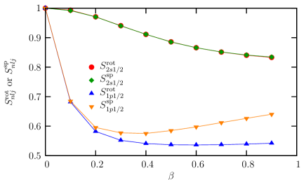
Figure 1: (color online) Spectroscopic factors $S^{\rm rot}_{nlj}$ (25) and single-particle approximation $S^{\rm sp}_{nlj}$ (15) as a function of deformation. Note that the diamonds are superimposed on the circles.

In Fig.1 we show the spectroscopic factors $S^{\rm rot}_{nlj}$ obtained from the solution of the coupled-channel equations as a function of deformation. Results for the g.s. (circles) and the e.s. (up triangles) are both included. The effect of deformation is very different in these two states although they are both loosely bound, and both correspond to a mixing of three configurations. The $S^{\rm rot}_{2s1/2}$ in the g.s. remains above $80$% even at large deformation. The remaining strength is shared between both $d$ configurations. On the contrary the $S^{\rm rot}_{1p1/2}$ in the e.s. drops rapidly with deformation down to 50–60%. The remaining part of the strength is exclusively in the $p3/2$ configuration. No strength is found in the $f5/2$ configuration. These results are in agreement with those of Refs. Nunes et al. (1996); Esbensen et al. (1995); Vinh Mau (1995). For both states, there is no configuration crossing: only one configuration dominates for all deformations. In both cases, the dependence of SFs on $\beta$ is strongly non-linear. Interestingly, at small $\beta$, and when there is little admixture, $1-S^{\rm rot}_{2s1/2}$ behaves roughly quadratically in $\beta$, as discussed at the end of Sec. II.4.

We compare these SFs with the values that would have been obtained under the single-particle approximation (15). For the g.s., this approximation (diamonds) works very well: no matter how large the coupling strength, $S^{\rm sp}_{2s1/2}\approx S^{\rm rot}_{2s1/2}$. For the e.s. (down triangles), only the general trend of $S^{\rm rot}_{1p1/2}$ is reproduced by $S^{\rm sp}_{1p1/2}$. Although the single-particle approximation is valid at small deformation significant discrepancies appears for $\beta>0.2$.

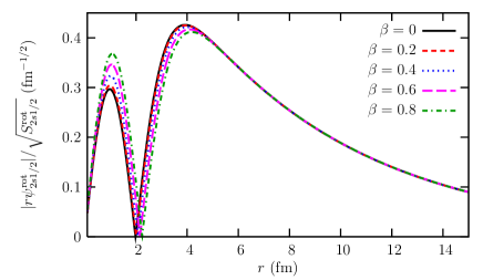
Figure 2: (color online) Radial part of $2s1/2$ overlap functions normalized to unity.

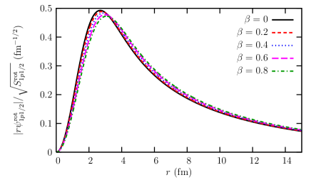
Figure 3: (color online) Radial part of $1p1/2$ overlap functions normalized to unity.

These results can be further illustrated by plotting the $2s1/2$ and $1p1/2$ components of the wave function for various deformation parameters (Figs. 2 and 3). These radial functions have been normalized to one to make the comparison easier. We see that the couplings simply rearrange the interior of the $s1/2$ contribution: increasing $\beta$ moves strength from the second peak to the first. However the asymptotic part (beyond 5 fm) is left totally unchanged, explaining the validity of the single-particle approximation (15). For this loosely-bound $1/2^{+}$ state, we find that 50% of the spectroscopic strength comes from radii smaller than the interaction radius. This illustrates that even for loosely-bound systems, the internal part of the overlap function significantly contributes to the SF. The validity of the single-particle approximation is therefore surprising. Although couplings significantly affect the interior of the overlap function, which contributes to a large part of the SF, the approximation (15), based solely on asymptotic characteristics of the wave function, gives a precise estimate of the SF.

As opposed to the $1/2^{+}$ state, the couplings seem to affect the wave function of the $1/2^{-}$ state all the way out to large distances (see Fig. 3). In this case, strength is moved outwards when $\beta$ increases. This explains the deviation between $S^{\rm rot}_{1p1/2}$ and its single-particle approximation $S^{\rm sp}_{1p1/2}$ observed in Fig. 1.

These results obtained for a realistic description of ¹¹Be are rather surprising. First, it was expected that at some point, e.g. for large deformation, the single-particle approximation would break down. However, as shown in Fig. 1, the single-particle approximation seems to be valid even at large $\beta$, especially for the ground state. Second, large differences are observed between the two states. For the ground state, the $2s1/2$ configuration dominates and the single-particle approximation is nearly exact. On the contrary, the excited state presents a large admixture of the $1p1/2$ and $1p3/2$ configurations, and the single-particle approximation of its SF is less precise.

The difference in the validity of the single-particle approximation (15) can be understood in terms of the different admixtures that are obtained in the g.s. and the e.s. This suggests that the single-particle approximation is less valid at large admixture, i.e. when the corresponding SF is small. This agrees, at least qualitatively, with the arguments expounded in the description of the delta-coupling model.

One possible explanation for the difference in the configuration admixture between both states is the presence of a bound state in the $p3/2$ partial wave generated by the core-neutron potential Capel et al. (2004). The existence of such a state could attract probability flux to that configuration and so enhance the admixture in the e.s. Accordingly, the low admixture observed in the g.s. would be explained by the absence of bound state in the $d$ waves. To better understand these results, we perform similar calculations extending the range of parameters to extreme values.

III.2 Extreme couplings

To study the difference in admixture observed between the two bound states, we perform calculations for a hypothetical g.s. of ¹¹Be with different values of $V_{d}$ to see if and when the presence of a bound state in the $d$ wave affects the admixture in that state. To do so, we repeat the analysis performed in Sec. III.1 for the g.s., but now, instead of adjusting $V_{d}$ to the resonant state, we use it as a free parameter and adjust $V_{s}$ to reproduce the correct g.s. energy. For simplicity, the spin of the neutron is neglected. Results are shown in Fig. 4(a) for deformation parameters $\beta=0.1$ (circles), 0.4 (squares), and 0.8 (diamonds). The most striking feature is the pronounced drop of $S^{\rm rot}_{2s}$ at $V_{d}\approx 80$ MeV. At this depth, the single-particle potential hosts a $d$ bound state with an energy that corresponds approximately to $\varepsilon^{Bn}_{1/2^{+}}-\epsilon_{2^{+}}$. In that condition, we have a nearly degenerate system, where the g.s. can be simultaneously in both $2s$ and $1d$ configurations. It is only the presence of this deep $d$ bound state that explains the large admixture. Indeed at lower or larger $V_{d}$, the admixture vanishes and $S^{\rm rot}_{2s}>0.8$. This behavior holds for all coupling strengths, though the region of large admixture increases with deformation $\beta$. Note also the discontinuity of our results, especially at large $\beta$. In the large-admixture range, parameters cannot be adjusted to reproduce the binding energy of the system due to numerical limitations.

This result confirms the hypothesis formulated at the end of Sec. III.1. It shows that large admixture is to be expected near degeneracy, i.e. when the coupled wave hosts a bound state close to the energy $\varepsilon^{Bn}_{J^{\pi}}-\epsilon_{I^{\pi_{B}}}$. However, if that bound state is located above or below that energy, no significant admixture should be observed. This explains the small admixture observed in the g.s. of the realistic ¹¹Be. In that case $V_{d}$ is adjusted to reproduce the $5/2^{+}$ resonance. In the single-particle potential, all $d$ states are thus in the continuum, far from the energy at which there would be degeneracy. The admixture observed in the e.s. of the realistic ¹¹Be is also explained by this effect. The single-particle parameters indeed lead fortuitously to a $1p3/2$ state bound by about $3$ MeV Capel et al. (2004), which corresponds approximately to $\varepsilon^{Bn}_{1/2^{-}}-\epsilon_{2^{+}}$, i.e. the energy at which there is degeneracy. Note that the large admixture observed in the e.s. of ¹¹Be is unphysical as the $p3/2$ orbital is Pauli blocked to the valence neutron Sagawa et al. (1993). Because of the large centrifugal barrier, the $1f5/2$ state is located high in the continuum, and so does not couple to the $p$ configurations.

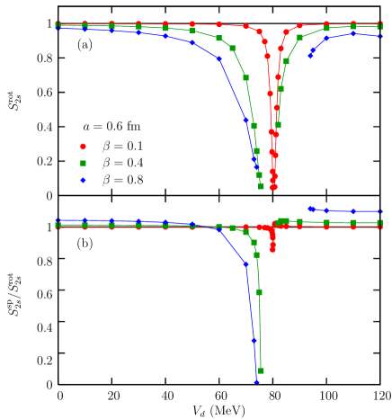
Figure 4: (color online) (a) Spectroscopic factors as a function of $V_{d}$. (b) Relative effect of the single-particle approximation as a function of $V_{d}$. ($a=0.6$ fm)

Besides aiding to understand the results obtained in Sec. III.1, these manipulations enable us to induce large admixture in our two-cluster rotational model. In this way we can study the validity of the single-particle approximation in nuclei with large fragmentation of strength that usually require more advanced structure models. In Fig. 4(b), the ratio of the single-particle estimate $S^{\rm sp}_{2s}$ (15) to its “exact” value $S^{\rm rot}_{2s}$ (25), is plotted as a function of $V_{d}$. The approximation works perfectly at small coupling strength and its validity decreases as $\beta$ increases. However, no matter how large the coupling strength, the single-particle approximation remains valid outside the large-admixture range with less than 10% error. This confirms that the single-particle approximation breaks down mostly at large admixture.

Fig. 5 shows the equivalent of Fig. 4 but for a much smaller diffuseness $a=0.1$ fm. We perform this set of calculation not only to test the validity of our conclusions in extreme cases, but also to ease the comparison between this rotational model and the delta-coupling model, which corresponds to a nil diffuseness (see Sec. III.3). In this case, the large-admixture range is increased. Therefore the breakdown of the single-particle approximation happens sooner and to a larger extent. This is due to the smaller diffuseness, which produces a more abrupt change in the radial behavior of the wave function at the surface and so enhances the couplings between the various configurations.

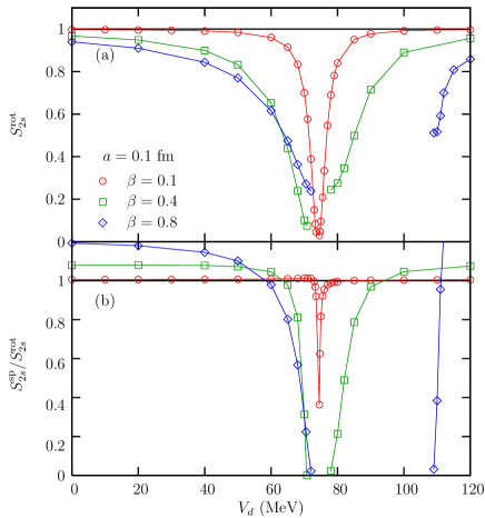
Figure 5: (color online) (a) Spectroscopic factors as a function of $V_{d}$. (b) Relative effect of the single-particle approximation as a function of $V_{d}$. ($a=0.1$ fm)

To summarize this analysis, we plot in Fig. 6 the single-particle approximation $S^{\rm sp}_{2s}$ against the “exact” $S^{\rm rot}_{2s}$ for all the cases explored in this section. These correspond to the deformations $\beta=0.1$, 0.4, and 0.8 (circles, squares, and diamonds, respectively) and two diffusenesses $a=0.1$, and 0.6 fm (open and solid symbols). The dashed line corresponds to $S^{\rm sp}_{2s}=S^{\rm rot}_{2s}$ and the deviation from this line estimates the error of the single-particle approximation. The main information conveyed by Fig. 6 is the general agreement between the “exact” SF and its single-particle approximation. Although there are some deviations from the $S^{\rm sp}_{2s}=S^{\rm rot}_{2s}$ line, a large $S^{\rm sp}_{2s}$ correctly predicts a large $S^{\rm rot}_{2s}$, while a small $S^{\rm sp}_{2s}$ is usually obtained for small $S^{\rm rot}_{2s}$. Besides this qualitative information, Fig.6 emphasizes the fact that for small coupling strengths, the agreement between $S^{\rm sp}_{2s}$ and $S^{\rm rot}_{2s}$ is excellent, even for large admixture with other configurations, i.e. for small SF. It also shows very clearly that the deviation becomes larger as the coupling strength $\beta$ increases. As noted earlier, this effect is more pronounced for smaller diffuseness.

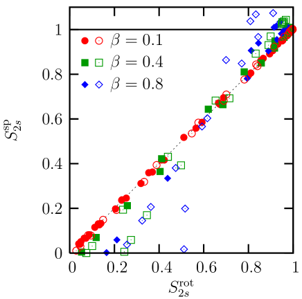
Figure 6: (color online) Comparing the single-particle approximation $S^{\rm sp}_{2s}$ to the “exact” $S^{\rm rot}_{2s}$. Closed symbols correspond to diffuseness $a=0.6$ fm, and open ones to $a=0.1$ fm.

The largest discrepancy between the prediction $S^{\rm sp}_{2s}$ and the “exact” $S^{\rm rot}_{2s}$ is observed for small SF, where the single-particle approximation tends to significantly underestimate the SF. To understand this effect, we display in Fig. 7 the radial component of some $2s$ overlap functions obtained in the most unfavorable case, i.e. $\beta=0.8$ and $a=0.1$ fm. These functions are labeled by the value of $V_{d}$ they correspond to (cf. Fig. 5). The single-particle wave function (i.e. $\beta=0$) is shown as well for comparison (thick full line). As already observed in Fig. 2, the couplings between the configurations affects the overlap function. In most of the cases these changes are limited to the interior of the overlap function, leaving the asymptotics (nearly) unchanged. However, for some extreme cases, they extend much beyond the range of the single-particle potential. In particular, the node of the overlap function may be pushed so much outwards that the ANC $C^{\rm rot}_{2s}$ nearly vanishes (see, e.g., $V_{d}=72$ MeV). This leads to the very small estimates $S^{\rm sp}_{2s}$ observed in Figs. 4(b), 5(b), and 6, whereas there remains some significant probability strength in the interior of the wave function, i.e., a non-zero $S^{\rm rot}_{2s}$. These rapid variations in the wave function also explain the difficulty in adjusting the parameters of the model within the large-admixture range (see Figs. 4 and 5). However, these extreme cases seem to occur only for a combination of large coupling strengths and significant admixture.

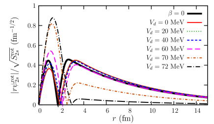
Figure 7: (color online) Radial part of the $s$ overlap functions normalized to unity obtained for $\beta=0.8$ and $a=0.1$ fm.

III.3 Analysis with the $\delta$ coupling

To expand our perspectives on the results obtained within the rotational model, we perform a similar analysis using the delta-coupling model developed in Sec. II.4. We consider here the g.s. of a ¹¹Be-like system. We take into account the main component $2s$ with the core in its $0^{+}$ ground state coupled to the $1d$ component with the core in its $2^{+}$ excited state. In a first step, the same square-well potential is taken in both $s$ and $d$ partial waves.

In Fig. 8 we show a plot equivalent to Fig. 1 for the delta-coupling model. We find that $S^{\delta}_{0}$ (solid line) decreases with the coupling strength $\beta$ to very small values. Note that the quadratic dependence of $1-S^{\delta}_{0}$ in $\beta$ is only observed for very small coupling strength, namely $\beta<0.02$. For $\beta>0.4$ the dominant component in the $1/2^{+}$ state is no longer the $2s$ component but the $1d$ one. This larger admixture as compared to the rotational model may be due to the node of the $2s$. In the rotational model, the combination of that node and the finite extension of the coupling potential might sufficiently reduce the source term in the $d$-wave equation to limit the admixture. On the contrary, the nil extension of the delta coupling avoids this cancellation effect, which could explain the larger admixture. Another explanation is the intrinsically larger coupling strength in the delta coupling due to its nil diffuseness. We have indeed seen in Sec. III.2 that decreasing the diffuseness increases the admixture between configurations (compare Figs. 4(a) and 5(a)). Whatever the reason for that larger admixture, it leads to a less reliable single-particle approximation (dashed line), as already seen in the rotational model. The $S^{\rm sp}_{0}$ now deviates significantly from the $S^{\delta}_{0}$ (the error can be as large as a factor of 2). Nevertheless, it reproduces qualitatively the general trend of the “exact” SF. Moreover, at small admixtures (i.e. for $S^{\delta}_{0}>80$%), the single-particle approximation is in perfect agreement with $S^{\delta}_{0}$.

Figure 8: Spectroscopic factors as a function of deformation for the delta-coupling model.

To confirm the degeneracy effect observed in the rotational model, we repeat the analysis performed in Sec. III.2: The depth of the square well in the $d$ wave $V_{d}$ is varied while the depth in the $s$ wave is adjusted to fit the ¹⁰Be-$n$ binding energy. The results of this analysis are displayed in Fig. 9, where $S^{\delta}_{0}$ is plotted as a function of $V_{d}$ for various coupling strengths $\beta=0.05$ (full line), 0.2 (dashed line), and 0.4 (dotted line). These results are very similar to those obtained for the rotational model, and in particular for the small diffuseness (see Fig. 5(a)). Little admixture is observed outside a range centered on $V_{d}\approx 75$ MeV, at which value the single-particle potential hosts a $d$ bound state at $\varepsilon^{Bn}-\epsilon_{2^{+}}$. As in the rotational model, the width of that large-admixture range increases with the coupling strength. We also observe discontinuities in the SF similar to those observed in Fig. 5(a). These results confirm the degeneracy effect observed in Sec. III.2: large admixture takes place when the potential well in the coupled channel is quantum-mechanically fit to host a bound state at the right energy. This effect seems therefore general and not due to some artefact of the rotational model.

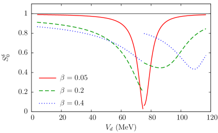
Figure 9: (color online) Spectroscopic factors as a function of $V_{d}$ for the delta-coupling model.

In Fig. 10, the single-particle approximation $S^{\rm sp}_{0}$ (15) is compared to the “exact” $S^{\delta}_{0}$ (31). This figure is very similar to Fig. 6. It confirms that the single-particle approximation predicts a SF in qualitative agreement with the “exact” one. The prediction is more reliable for small admixture, i.e. large SF, as already seen in Fig. 6. At these values, the discrepancy between the “exact” SF and its single-particle approximation roughly follows

$$S^{\delta}_{0}-S^{\rm sp}_{0}\propto 1-S^{\delta}_{0},$$ (32)

in agreement with the reasoning of Sec. II.4. This error increases with the coupling strength $\beta$. Note that a similar, though less obvious, result is observed in Fig. 6.

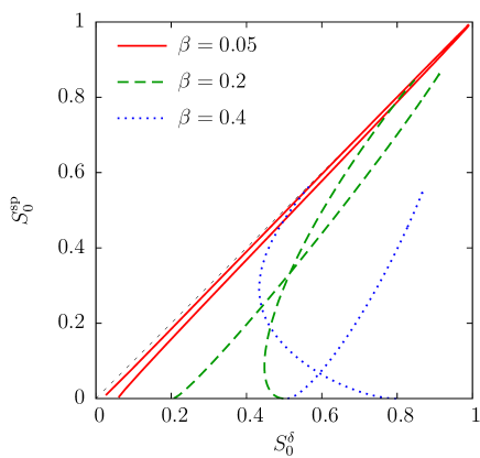
Figure 10: (color online) Comparison of the single-particle approximation $S^{\rm sp}_{0}$ (15) with the SF obtained within the delta-coupling model $S^{\delta}_{0}$ (31).

IV Discussion and Conclusions

Spectroscopic information about exotic nuclear structures, like halo nuclei, can be inferred from direct reactions Roussel-Chomaz (2010); Thomas et al. (2007); Hansen and Tostevin (2003); Nakamura et al. (1999). Usually a SF and/or an ANC are extracted from the analysis of these experiments. Most of these analyses are performed within a single-particle approximation of the projectile wave function. In order to evaluate the validity of this approximation, we have studied the influence of coupling between configurations upon the overlap wave function. Keeping in mind the extraction of SF from peripheral reactions Mukhamedzhanov and Nunes (2005); Capel and Nunes (2007), we have focused our study on the effects of these couplings on the SF and the ANC. Assuming that an ANC can be reliably extracted from direct reactions, we have analyzed how accurately a SF can be deduced from it.

In this work, we have considered a collective model of the nucleus in which a valence neutron is bound to a deformed core allowed to excite. In particular, we have used the rotational-coupling model of Nunes et al. Nunes et al. (1996); Thompson et al. (2004), in which the core is described as a deformed rotor. In this model the various states of the core are assumed to be part of a rotational band. A qualitative delta-coupling model has also been used to investigate the results of the rotational model. Calculations have been performed in the case of the typical one-neutron halo nucleus ¹¹Be.

Interestingly, this analysis shows that even a small coupling may affect significantly the overlap function. However, the changes compared to the single-particle wave function appear mostly in the interior, leaving the asymptotics nearly unchanged (see Fig. 2). This surprising result suggests that probing only the tail of the wave function may give a reasonable estimate of the SF, contrarily to what has been assumed in LABEL:CN07. To explore this idea, we vary the deformation of the core that acts as a coupling strength. The single-particle approximation (15) is then compared to the “exact” SF obtained within the rotational model. This approximation is obtained from the ratio between the ANC of the rotational-coupling model and that of the single-particle model. The former acts as the actual ANC of the system, supposedly measured from peripheral reactions. The latter corresponds to the one obtained with a single-particle description of the nucleus, which is used in most of the reaction models. The prescription (15) therefore simulates the procedure performed in extracting SFs from experimental data.

The results of our analysis show that the single-particle approximation often provides a reliable estimate of the SF. This estimate is at least in qualitative agreement with the coupled-channel models: It predicts large (respectively small) SFs, when large (respectively small) SFs are obtained from the coupled-channel models. For very small coupling strength, this estimate is very accurate. On the contrary, for large coupling strength, and in particular for large admixture of the configurations, i.e. small SF, the single-particle approximation is much less reliable.

Being obtained within two independent structure models, this result seems quite general. To understand it on firmer grounds, let us look back at the coupled equations satisfied by the overlap function (10) and compare them with the single-particle equation (12). The overlap function $\psi_{\nu_{A}\nu_{B}}$ will depart from its single-particle approximation only when the coupling terms in Eq. (10) become significant, i.e. when at least one of the products $V_{\nu_{B}\mu_{B}}\psi_{\nu_{A}\mu_{B}}$ is large. This will happen for large coupling strengths, and/or when the population of the $\nu_{A}\mu_{B}$ configuration is large in the range of $V_{\nu_{B}\mu_{B}}$, i.e. when there is a significant admixture between the various channels. In these two cases, the coupling affects the overlap function so much that the single-particle approximation no longer holds. This reasoning also illustrates the possible influence of a node in one of the overlap function upon the admixture. Such a node may indeed cancel out the effect of the coupling if it is located within the range of $V_{\nu_{B}\mu_{B}}$. In the future, we plan to further investigate this effect.

This study suggests the simple rule of thumb that large SFs deduced from ANCs are reliable. On the contrary, single-particle analysis of data estimating small SF, i.e. a large admixture between configurations, should not be relied on. Note that in any case some uncertainty remains, and that even large SF estimates can be off by 10–20%. Therefore, these estimates must be taken for what they are—estimates—and not precise, unquestionable values.

The accuracy of the single-particle approximation depends also on the geometry of the potential chosen to simulate the mean field of the core. In practice this geometry is unknown. We have not considered this uncertainty in the present analysis. Fortunately, as observed by Sparenberg et al. Sparenberg et al. (2010), the single-particle ANC for loosely-bound states is not strongly dependent on the potential geometry. In particular for an $s$ valence neutron, it can be efficiently estimated from only the binding energy of the system (see Eq. (20) of LABEL:SCB10).

In our study, we consider a collective model to simulate microscopic effects. To evaluate the sensitivity of our conclusions to this approximation, it would be interesting to repeat this analysis with microscopic models, such as the microscopic cluster model Baye et al. (1994), the fermionic molecular dynamics Neff et al. (2005); Neff and Feldmeier (2008), or the Green’s function Monte Carlo model Pieper and Wiringa (2001), which all can correctly describe the asympotics of overlap wave functions for loosely-bound nuclear systems.

Appendix A Effective Hamiltonian in a single-particle equation

Given the linearity of the set of equations (10) for the overlap functions, any overlap function is linear in any other of those functions. Any selected equation may be then formally closed by expressing other overlap functions in terms of the function of interest. The cost is in a potentially strong nonlocality, both in position and energy, for the effective Hamiltonian within the single-particle equation for the chosen overlap function. Also, it may be difficult to construct the effective Hamiltonian in practice.

Let the chosen overlap function correspond to the state $\nu_{B}$ of the core $B$. First, energy eigenvectors need to be found in the remaining space of overlap functions, in the absence of coupling to $\nu_{B}$. With different energy values and eigenvectors denoted with index $\alpha$, an eigenvector $\eta^{\overline{\nu}_{B}\,\alpha}$ solves the set for energy $E^{\overline{\nu}_{B}\,\alpha}$,

$$\big{(}E^{\overline{\nu}_{B}\,\alpha}-\epsilon_{\mu_{B}}\big{)}\,\eta_{\mu_{B}}^{\overline{\nu}_{B}\,\alpha}=t_{\mbox{\boldmath$r$}}\,\eta_{\mu_{B}}^{\overline{\nu}_{B}\,\alpha} +\sum_{\gamma_{B}\neq\nu_{B}}V_{\mu_{B}\,\gamma_{B}}\,\eta_{\gamma_{B}}^{\overline{\nu}_{B}\,\alpha}\,,$$

$$(\text{for}\;\mu_{B}\neq\nu_{B})\,.$$ (33)

Note that, without the coupling potentials $V_{\mu_{B}\,\gamma_{B}}$, the states $\{\eta^{\overline{\nu}_{B}\,\alpha}\}$ would just represent energy eigenstates within the single-particle potential, coming in near-degenerate sets, because of the expected weak-dependence of the potential on $\mu_{B}$. Given the coupling to $\psi_{\nu_{A}\nu_{B}}$ of the overlap functions $\psi_{\nu_{A}\,\mu_{B}}$, where $\mu_{B}\neq\nu_{B}$, the set of the latter functions can be next expressed as a combination of the vectors $\{\eta^{\overline{\nu}_{B}\,\alpha}\}$. Upon inserting the expressions for the functions $\psi_{\nu_{A}\,\mu_{B}}$ into the equation for the overlap function $\psi_{\nu_{A}\nu_{B}}$, we arrive at the closed equation:

$$\big{(}\varepsilon_{\nu_{A}}^{Bn}-\epsilon_{\nu_{B}}\big{)} \,\psi_{\nu_{A}\nu_{B}}({\boldsymbol{r}})=\Big{(}t_{\mbox{\boldmath$r$}}+V_{\nu_{B}\,\nu_{B}}({\boldsymbol{r}})\Big{)}\,\psi_{\nu_{A}\nu_{B}}({\boldsymbol{r}})$$

$$+\int d{\boldsymbol{r}}^{\prime}\,\Delta V_{\nu_{B}\,\nu_{B}}({\boldsymbol{r}},{\boldsymbol{r}}^{\prime};\varepsilon_{\nu_{A}}^{Bn})\,\psi_{\nu_{A}\nu_{B}}({\boldsymbol{r}}^{\prime})\,,$$ (34)

where the modification of the single-particle potential is

$$\Delta V_{\nu_{B}\,\nu_{B}}({\boldsymbol{r}},{\boldsymbol{r}}^{\prime};E)= \sum_{\begin{subarray}{c}\mu_{B}\neq\nu_{B}\\ \gamma_{B}\neq\nu_{B}\end{subarray}}V_{\nu_{B}\,\mu_{B}}({\boldsymbol{r}})$$

$$\times G_{\mu_{B}\,\gamma_{B}}^{\overline{\nu}_{B}}({\boldsymbol{r}},{\boldsymbol{r}}^{\prime};E)\,V_{\gamma_{B}\,\nu_{B}}({\boldsymbol{r}}^{\prime})\,,$$ (35)

and the Green’s propagator within the space complementary to $\nu_{B}$ is

$$G_{\mu_{B}\,\gamma_{B}}^{\overline{\nu}_{B}}({\boldsymbol{r}},{\boldsymbol{r}}^{\prime};E)= \sum_{\alpha}\frac{1}{E-E^{\overline{\nu_{B}}\alpha}}$$

$$\quad\quad\times\eta_{\mu_{B}}^{\overline{\nu}_{B}\,\alpha}({\boldsymbol{r}})\,\left[\eta_{\gamma_{B}}^{\overline{\nu}_{B}\,\alpha}({\boldsymbol{r}}^{\prime})\right]^{*}\,.$$ (36)

The results are written here assuming local 2-body interactions.

The nature of the contributions to the Green’s function, and to the modification of the potential $\Delta V$, from different excitations of the core, will depend on the core excitation energy. High-lying excitations will yield contributions where propagation both to the outside and inside of the nucleus represents a tunneling. Those contributions will not yield much nonlocality for $\Delta V$, neither as a function of position nor energy. On the other hand, for low-lying excitations, the propagation within the nuclear volume may be largely uninhibited, while still turning to tunneling in the exterior. The latter excitations will contribute nonlocalities to $\Delta V$, both in terms of energy-dependence and position, with latter nonlocalities possibly extending across the nucleus. The different limits of nonlocality may be, in particular, easily assessed in the delta-coupling model. In this paper, the focus is on the impact of coupling to low-lying states, on the overlap functions and on the deduced SFs. We may mention, though, that many microscopic interactions $v_{ij}$ with strong short-range repulsion may yield unphysical single-particle potential $V_{\nu_{B}\,\nu_{B}}$ in absence of any modification in the form of $\Delta V$. For such interactions, some level of renormalization of the potentials $V_{\nu_{B}\,\mu_{B}}$, for low-lying states, through coupling to high-lying states may be necessary to start with. The consequence in the possible ill-definition of SFs, due to the latter type of couplings, has been indicated in Ref. Furnstahl and Hammer (2002).

References

- Fulton (2010) B. Fulton, in Proc. of the International Nuclear Physics Conference, edited by J. Thomson and J. Dilling (Institute of Physics, Vancouver, Canada, 2010), pp. –, to be published in the J. Phys.: Conf. Series.
- Roussel-Chomaz (2010) P. Roussel-Chomaz, in Proc. of the International Nuclear Physics Conference, edited by J. Thomson and J. Dilling (Institute of Physics, Vancouver, Canada, 2010), pp. –, to be published in the J. Phys.: Conf. Series.
- Thomas et al. (2007) J. S. Thomas, G. Arbanas, D. W. Bardayan, J. C. Blackmon, J. A. Cizewski, D. J. Dean, R. P. Fitzgerald, U. Greife, C. J. Gross, M. S. Johnson, et al., Phys. Rev. C 76, 044302 (2007).
- Hansen and Tostevin (2003) P. G. Hansen and J. A. Tostevin, Annu. Rev. Nucl. Part. Sci. 53, 219 (2003).
- Nakamura et al. (1999) T. Nakamura, N. Fukuda, T. Kobayashi, N. Aoi, H. Iwasaki, T. Kubo, A. Mengoni, M. Notani, H. Otsu, H. Sakurai, et al., Phys. Rev. Lett. 83, 1112 (1999).
- Thompson and Nunes (2009) I. Thompson and F. Nunes, Nuclear reactions for astrophysics (University Cambridge Press, U.K., 2009).
- Furnstahl and Hammer (2002) R. J. Furnstahl and H. W. Hammer, Phys. Lett. B 531, 203 (2002).
- Furnstahl and Schwenk (2010) R. Furnstahl and A. Schwenk, J. Phys. G 37, 064005 (2010).
- Mukhamedzhanov and Nunes (2005) A. M. Mukhamedzhanov and F. M. Nunes, Phys. Rev. C 72, 017602 (2005).
- Capel and Nunes (2007) P. Capel and F. M. Nunes, Phys. Rev. C 75, 054609 (2007).
- Nunes et al. (1996) F. M. Nunes, I. J. Thompson, and R. C. Johnson, Nucl. Phys. A 596, 171 (1996).
- Thompson et al. (2004) I. J. Thompson, F. M. Nunes, and B. V. Danilin, Comput. Phys. Commun. 161, 87 (2004).
- Esbensen et al. (1995) H. Esbensen, B. A. Brown, and H. Sagawa, Phys. Rev. C 51, 1274 (1995).
- Vinh Mau (1995) N. Vinh Mau, Nucl. Phys. A 592, 33 (1995).
- Pang et al. (2007) D. Y. Pang, F. M. Nunes, and A. M. Mukhamedzhanov, Phys. Rev. C 75, 024601 (2007).
- Mukhamedzhanov et al. (2008) A. M. Mukhamedzhanov, F. M. Nunes, and P. Mohr, Phys. Rev. C 77, 051601 (2008).
- Dickhoff and Barbieri (2004) W. H. Dickhoff and C. Barbieri, Prog. Part. Nucl. Phys. 52, 377 (2004).
- Summers et al. (2006a) N. C. Summers, F. M. Nunes, and I. J. Thompson, Phys. Rev. C 73, 031603 (2006a).
- Summers et al. (2006b) N. C. Summers, F. M. Nunes, and I. J. Thompson, Phys. Rev. C 74, 014606 (2006b).
- Matsumoto et al. (2006) T. Matsumoto, T. Egami, K. Ogata, Y. Iseri, M. Kamimura, and M. Yahiro, Phys. Rev. C 73, 051602 (2006).
- Rodríguez-Gallardo et al. (2008) M. Rodríguez-Gallardo, J. M. Arias, J. Gómez-Camacho, R. C. Johnson, A. M. Moro, I. J. Thompson, and J. A. Tostevin, Phys. Rev. C 77, 064609 (2008).
- Baye et al. (2009) D. Baye, P. Capel, P. Descouvemont, and Y. Suzuki, Phys. Rev. C 79, 024607 (2009).
- Pieper and Wiringa (2001) S. C. Pieper and R. B. Wiringa, Annu. Rev. Nucl. Part. Sci. 51, 53 (2001).
- Forssén et al. (2008) C. Forssén, J. P. Vary, E. Caurier, and P. Navrátil, Phys. Rev. C 77, 024301 (2008).
- Quaglioni and Navrátil (2009) S. Quaglioni and P. Navrátil, Phys. Rev. C 79, 044606 (2009).
- Timofeyuk (2010) N. K. Timofeyuk, Phys. Rev. C 81, 064306 (2010).
- Brida and Nunes (2010) I. Brida and F. Nunes, Nucl. Phys. A 847, 1 (2010).
- Abramowitz and Stegun (1970) M. Abramowitz and I. A. Stegun, Handbook of Mathematical Functions (Dover, New-York, 1970).
- Capel et al. (2004) P. Capel, G. Goldstein, and D. Baye, Phys. Rev. C 70, 064605 (2004).
- Sagawa et al. (1993) H. Sagawa, B. A. Brown, and H. Esbensen, Phys. Lett. B 309, 1 (1993).
- Sparenberg et al. (2010) J.-M. Sparenberg, P. Capel, and D. Baye, Phys. Rev. C 81, 011601 (2010).
- Baye et al. (1994) D. Baye, P. Descouvemont, and N. K. Timofeyuk, Nucl. Phys. A 577, 624 (1994).
- Neff et al. (2005) T. Neff, H. Feldmeier, and R. Roth, Nucl. Phys. A 752, 321 (2005).
- Neff and Feldmeier (2008) T. Neff and H. Feldmeier, Eur. Phys. J. Special Topics 156, 69 (2008).