High Order Coherent Control Sequences of Finite-Width Pulses

Abstract

The performance of sequences of designed pulses of finite length $\tau$ is analyzed for a bath of spins and it is compared with that of sequences of ideal, instantaneous pulses. The degree of the design of the pulse strongly affects the performance of the sequences. Non-equidistant, adapted sequences of pulses, which equal instantaneous ones up to $\mathcal{O}(\tau^{3})$, outperform equidistant or concatenated sequences. Moreover, they do so at low energy cost which grows only logarithmically with the number of pulses, in contrast to standard pulses with linear growth.

The rapid evolution of the field of quantum science and quantum information demands robust quantum control techniques in the presence of environmental noise. To dynamically generate systems essentially free from decoherence has now become a focus of the research of quantum control. This suppression of decoherence is an important requisite in quantum information processing Nielsen and Chuang (2000), for example for the realization of a quantum computer, in nuclear magnetic resonance (NMR), for high accuracy measurements Haeberlen (1976) or in magnetic resonance imaging (MRI) Jenista et al. (2009), to mention only a few.

In this work we focus on quantum control by short pulses of finite length. It is beyond our scope to discuss continuous quantum control, see for instance Ref. Gordon et al., 2008. It is on a discovery in NMR, the Hahn spin echo Hahn (1950), that the pulsed-control methods are based. The original technique makes use of an electromagnetic pulse in order to rotate the spin and to refocus it along a desired direction. Dynamical decoupling (DD) Viola and Lloyd (1998); Ban (1998) iterates the single pulse in a sequence of pulses such that the coupling between the spin and its environment is averaged to zero. Among the “open-loop” pulse-control techniques, the dynamical decoupling is one of the most promising protocols for prolonging the coherence time of a spin (qubit) coupled to an environment. No detailed, quantitative knowledge of the decohering environment is required.

The sequences come in a large variety. We distinguish equidistant and non-equidistant sequences. In the first category we recall the iterated Carr-Purcell-Meiboom-Gill (CPMG) sequence Carr and Purcell (1954); Meiboom and Gill (1958), where the pulses are regularly separated (apart from the very first and the very last one). To the second category belong for instance the universal Uhrig DD (UDD) sequence Uhrig (2007); Lee et al. (2008); Yang and Liu (2008), the Locally Optimized Dynamical Decoupling (LODD) Biercuk et al. (2009), the Optimized Noise Filtration by Dynamical Decoupling (OFDD) Uys et al. (2009) and the Bandwidth-Adapted Dynamical Decoupling (BADD) Khodjasteh et al. (2011) for pure dephasing models and the concatenated DD (CDD) Khodjasteh and Lidar (2005) or UDD (CUDD) Uhrig (2009) or the quadratic UDD (QDD) West et al. (2010) for models with dephasing and relaxation.

The design of the DD schemes relies originally on the assumption that the pulses are arbitrarily strong and instantaneous though the effects of pulses of finite length were known to matter Skinner et al. (2003); Viola and Knill (2003); Sengupta and Pryadko (2005); Khodjasteh and Lidar (2007); Pryadko and Quiroz (2008). But the pulses used in laboratories always have a bounded, finite amplitude so that they have a finite duration $\tau$. Even if sequences like CPMG and UDD have already been implemented in experiments with very good results Biercuk et al. (2009); Du et al. (2009); Jenista et al. (2009), the fact that pulses have a finite duration appears often as a nuisance deteriorating the suppression of decoherence, see for instance Refs. Viola and Knill, 2003 and Khodjasteh and Lidar, 2007.

It is of great practical relevance to which extent the length of a pulse affects the performance of a sequence such as UDD or CPMG of given duration $T$. How should one choose the location, the duration (or the amplitude), and the shape Sengupta and Pryadko (2005); Pryadko and Quiroz (2008); Pasini et al. (2009) of the bounded pulse in order to minimize the errors due to its finite duration if it replaces the ideal, instantaneous pulses in a certain sequence?

Here we report for the first time numerical evidence of how sequences of realistic pulses of finite width must be designed in order to achieve the same perturbative suppression of dephasing as the corresponding ideal sequence. We compare various known sequences Viola and Knill (2003); Khodjasteh and Viola (2009); Uhrig and Pasini (2010) and numerically analyze their performance for a spin coupled to a bath of spins. To obtain an experimentally relevant comparison all pulses are designed in such a way that the largest amplitude appearing in each sequence is the same enr .

The Model.

We consider the pure dephasing Hamiltonian $H=1_{q}\otimes B_{0}+\sigma_{z}\otimes B_{z}$ that determines the free evolution of the system between two consecutive pulses by $U_{\mathrm{free}}(t)=\exp\{-itH\}$. The operators $B_{0}$ and $B_{z}$ act on the bath only, while the identity $1_{q}$ and the Pauli matrix $\sigma_{z}$ act on the qubit represented by a spin $1/2$. For simplicity we identify henceforth $1_{q}\otimes B_{0}$ and $B_{0}$. The bath consists of $M$ spins with $i\in\{1,\ldots,M\}$

$$H=\omega_{\mathrm{b}}B_{0}+\sigma^{(0)}_{z}\sum_{i=1}^{N_{s}}\lambda_{i}\ \sigma_{z}^{(i)}.$$ (1)

No drift term $\propto\sigma_{z}$ of the qubit is included because we work in the rotating reference frame. Explicitly we analyze two cases, see also Fig. 1: (i) A spin chain with $B_{0}=\sum_{i=1}^{M}\vec{\sigma}^{(i)}\cdot\vec{\sigma}^{(i+1)}$, $\lambda_{i}\equiv\lambda$ and $N_{s}=1$. (ii) A central spin model Schliemann et al. (2003); Bortz and Stolze (2006, 2007); Witzel and Das Sarma (2008); Lee et al. (2008); Witzel et al. (2007) characterized by a dipolar coupling Haeberlen (1976) $B_{0}=\sum_{j<i=1}^{M}\left(3\sigma_{z}^{(i)}\sigma_{z}^{(j)}-\vec{\sigma}^{(i)}\cdot\vec{\sigma}^{(j)}\right)$ with $\lambda_{i}(M-1)=\lambda(2i-M-1)$ and $N_{s}=M$. The rapidity of the dynamics of the bath is given by $\omega_{\mathrm{b}}:=\alpha\lambda$ with $\alpha$ a dimensionless constant.

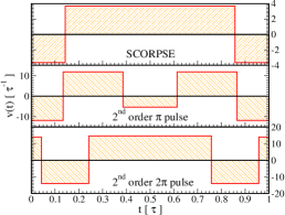
Figure 1: Left: Spin bath models under study with a qubit (square) coupled (dashed lines) to $M$ bath spins (dots) interacting among themselves (solid lines). Right: Upper panel: 1${}^{\text{st}}$ order SCORPSE $\pi$ pulse Cummins et al. (2003); middle panel: 2${}^{\text{nd}}$ order $\pi$ pulse; lower panel: 2${}^{\text{nd}}$ order $2\pi$ pulse. Both 2${}^{\text{nd}}$ order pulses are found by solving the conditions derived in Ref. Pasini et al., 2009. Amplitudes and switching instants are available upon request.

The control Hamiltonian is given by $H_{\mathrm{c}}(t)=\sigma_{x}^{0}v(t)$. We consider piecewise constant pulses shown in Fig. 1. During each pulse of total length $\tau^{(i)}$ the qubit evolves under the simultaneous action of the system and of the control Hamiltonian $U_{\mathrm{p}}={\cal T}\exp\{-i\int_{t_{0}}^{t_{0}+\tau^{(i)}}(H+H_{\mathrm{c}}(t))dt\}$ where ${\cal T}$ stands for standard time ordering. The evolution operator of the total sequence from $t=0$ to $t=T$ is denoted by $\widehat{R}$.

The Sequences.

Two types of sequences are studied, see also Fig. 2: (i) The durations $\tau^{(i)}=\tau^{*}$ of the pulses is constant throughout the sequence and it is kept constant on variation of $T$. These sequences are denoted by $\tau_{j}$CPMG, $\tau_{j}$CDD and $\tau_{j}$UDD, because they reproduce the ideal CPMG, CDD and UDD sequences for $\tau\rightarrow 0$. The subscript $j$ stands for properties of the pulses as explained below. (ii) The durations $\tau^{(i)}$ are varied along the sequence, i.e., they depend on $i$. But they shall not depend on $T$ other than that the sum of all pulse durations cannot exceed $T$, i.e., $T\geq T_{\text{p}}:=\sum_{i}\tau^{(i)}$. The corresponding sequences are denoted by $\tau_{j}$RUDD.

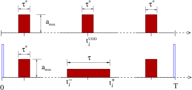
Figure 2: (Color online) Upper panel: Sequences of type (i) ($\tau_{j}$CPMG, $\tau_{j}$CDD or $\tau_{j}$UDD) are sketched. Lower panel: Sequences of type (ii) are shown ($\tau_{j}$RUDD). Only the maximum amplitude and the pulse duration are shown, but no details of the pulse shapes. The $\pi$-pulses are depicted by filled (red) blocks, the initial and final $2\pi$-pulses by open (blue) blocks. The first $\pi$ pulse of $\tau_{j}$RUDD and all pulses of type (i) sequences have the same amplitude $a_{\mathrm{max}}$ to ensure experimentally relevant comparability. The instants $t_{i}$ are given in Eqs. 2 and 3; the start and end points $t_{i}^{\pm}$ in Eq. (4).

The sequences of type (i) are made of $N$ $\pi$ pulses whose width is $\tau^{*}$. The center of the $i$-th pulse is given by

$$t_{i}^{\text{CPMG}}:=T\ (2i-1)/(2N),$$ (2a)

$$t_{i}^{\text{UDD}}:=T\ \sin^{2}\left(\pi\,i/(2(N+1))\right),$$ (2b)

for the $\tau_{j}$CPMG and $\tau_{j}$UDD Uhrig (2007) sequence, respectively. We use the simplified version of CDD designed only for pure dephasing. The CDD sequence of level $k$ is defined by the recursion

$$\text{CDD}_{k+1}(T)=\text{CDD}_{k}\left({T/2}\right)\circ\Pi_{\pi}\circ\text{CDD}_{k}\left({T/2}\right),\\$$ (3a)

$$\text{CDD}_{k+1}(T)=\text{CDD}_{k}\left({T/2}\right)\circ\text{CDD}_{k}\left({T/2}\right),$$ (3b)

where (3a) holds for $k$ even and (3b) for $k$ odd; $\circ$ stands for concatenation and $\Pi_{\varphi}$ for the operator of a pulse of angle $\varphi$. The zero-level CDD${}_{0}(T)$ is free evolution without pulses.

The subscript $j$ in $\tau_{j}$ refers to the order of the pulses, i.e., its time evolution operator fulfills $U_{\mathrm{p}}=\exp\{-i\tau B_{0}\}\Pi_{\varphi}+\mathcal{O}(\tau^{j+1})$. We restrict our study here to explicit pulses with $j=0,1,2$, see Fig. 1, which fulfill the conditions derived in Ref. Pasini et al., 2009. A recursion for general $j$ is given in Ref. Khodjasteh et al., 2010. The 0${}^{\text{th}}$ order pulse is simply rectangular; the other pulses used are depicted in Fig. 1.

The sequences of type (ii) are similar to the $\tau_{j}$UDD sequences in that they are based on pulses of order $j$. The crucial difference is that pulses are not constant in length. They are defined according to our previous work Uhrig and Pasini (2010) by a start instant $t_{i}^{-}$ and a stop instant $t_{i}^{+}$ given by

$$t^{\pm}_{i}:=T\sin^{2}\left(\frac{\pi\ i}{2(N+1)}\pm\frac{\theta_{\mathrm{p}}(T)}{2}\right).$$ (4)

The above relation results naturally from the requirement that the effective switching function of the sequence expressed in $\theta\in[0,\pi]$ according to $t=T\sin^{2}(\theta/2)$ is antiperiodic Uhrig and Pasini (2010). This antiperiodicity ensures that the total sequence suppresses the decohering terms $\propto\sigma_{z}$ in the time evolution Yang and Liu (2008). The duration of the pulses in time $\tau^{(i)}=t^{+}_{i}-t^{-}_{i}$ yielding

$$\tau^{(i)}=T\sin\left(\pi\ i/(N+1)\right)\sin(\theta_{\mathrm{p}})$$ (5)

is determined by the parameter $\theta_{\mathrm{p}}(T)$. It acquires a dependence on $T$ if we require $\tau^{*}:=\tau^{(1)}$ to be constant upon varying $T$. Note that $\theta_{\mathrm{p}}=\pi/(2(N+1))$ refers to back-to-back pulses without any free evolution between them, see below.

The antiperiodicity of the switching function is the basis for the suppression of dephasing in high order Yang and Liu (2008); Uhrig and Lidar (2010). In order to guarantee this antiperiodicity, it is required to insert an initial and a final pulse which represent the identity $U_{\mathrm{p}}=\exp\{-i\tau B_{0}\}+\mathcal{O}(\tau^{j+1})$. For instance, it may be a zero $\pi$ or a $2\pi$ pulse Uhrig and Pasini (2010). The initial pulse starts at $t_{0}^{-}=0$ and stops at $t_{0}^{+}=T\sin^{2}\left(\theta_{\mathrm{p}}/2\right)$ while the final one starts at $t_{N+1}^{-}=T\sin^{2}\left[(\pi-\theta_{\mathrm{p}})/2\right]$ and stops at $t_{N+1}^{+}=T$. These pulses are indicated by open boxes in Fig. 2.

In the sequel, we compare the various sequences always with the same $\tau^{*}$ because the shortest accessible pulse duration of a $\pi$ pulse, corresponding to the maximum amplitude, represents a crucial experimental constraint enr ; Khodjasteh et al. (2011). Only the very short boundary $2\pi$ pulses in the $\tau_{j}$RUDD are treated separately. But their importance is assessed by considering $\tau_{j}$RUDD with and without the boundary $2\pi$ pulses. We stress that due to the variable duration of the pulses according to (4,5) in the RUDD sequence most of the pulses are much longer than $\tau^{*}$.

The Partial Frobenius ($\Delta_{\mathrm{pF}}$) Distance

defines the distance between the ideal evolution of the initial state of the qubit due to the pulses and its evolution including the interaction with the bath and the application of the sequence Lidar et al. (2008). For each axis of rotation $\gamma=\{x,y,z\}$ we define a difference of density matrices of the qubit by $\rho_{\mathrm{q}}^{(\gamma)}:=\mathrm{tr_{B}}\left[\rho_{\mathrm{id}}^{(\gamma)}-\rho_{\mathrm{qB}}^{(\gamma)}\right]$, where $\rho_{\mathrm{qB}}^{(\gamma)}:=\widehat{R}\rho_{0}^{(\gamma)}\widehat{R}^{\dagger}$. The partial trace over the bath is denoted by $\mathrm{tr_{B}}$. Given a factorized initial state $\rho_{0}^{(\gamma)}:=|\gamma\rangle\langle\gamma|\otimes 1_{\mathrm{B}}$ the density matrix $\rho_{\mathrm{id}}^{(\gamma)}:=\sigma_{x}^{N}\rho_{0}^{(\gamma)}\sigma_{x}^{N}$ is the ideally evolved $\rho_{0}$ subject only to ideal pulses without any bath interaction. The distance $\Delta_{\mathrm{pF}}$ measures the difference between the real evolution and the ideal one reading

$$\Delta_{\mathrm{pF}}^{2}:={\frac{1}{3}\sum_{\gamma=x,y,z}\mathrm{tr_{q}}\left[\rho_{\mathrm{q}}^{(\gamma)}\right]^{2}}.$$ (6)

Numerical Simulation.

We compute the performance of sequences of pulses of finite duration for the systems in (1) shown in Fig. 1. We choose the minimum duration $\tau^{*}<\min_{i}\{\tau^{(i)}\}$ and a minimum value of $T$ such that $T\geq\sum_{i}\tau^{(i)}$, see captions for values. Sequences with $N=10$ pulses are considered because this number allows us to consider the CDD sequence as well; it corresponds to the concatenation level $k=4$, cf.  Eq. (3). The results are shown in Figs. 3 and 4(a) for the spin chain model and in Figs. 4(b) and Fig. 5 for the central spin model.

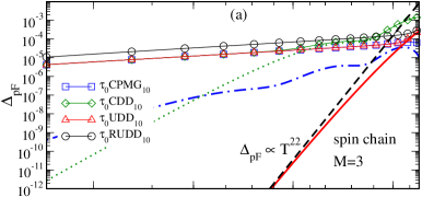
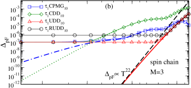
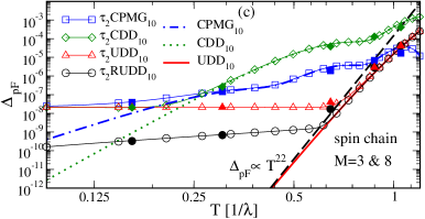
Figure 3: (Color online) Distance $\Delta_{\mathrm{pF}}$ vs. the duration $T$ of sequences of pulses with zero or finite width for $\alpha=10$ for spin chains. All open symbols refer to $M=3$ bath spins; the filled symbols in panel (c) to $M=8$ bath spins. The finite-width pulses have minimum width $\tau^{*}=1.086\cdot 10^{-3}/\lambda$ and $T\geq 0.09/\lambda$; Panel (a): rectangular 0^th order pulses; Panel (b): SCORPSE 1^st order pulses Cummins et al. (2003); Panel (c): 2^nd order pulses shown in Fig. 1. To highlight power-law behavior the dashed lines are included: The UDD curve scales as $T^{2(N+1)}$.

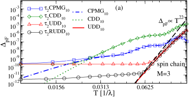
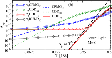
Figure 4: (Color online) Same as in Fig. 3(c). Panel (a): spin chain with $M=3$, $\alpha=100$ and $\tau^{*}=1.086\cdot 10^{-4}/\lambda$, $T\geq 0.009/\lambda$. Panel (b): central spin model with $M=8$, $\alpha=10$ and $\tau^{*}=0.0004828/\lambda$, $T\geq 0.04/\lambda$. The result is identical to Fig. 3(c) except for a shift by the factor $\kappa\approx 2.3$ in $T$.

First, we consider the influence of the topology and the size of the spin bath. In Fig. 3(c) data for the spin chain is shown for $M=3$ (open symbols) and data for $M=8$ (filled symbols) fits in perfectly. This indicates that the size effect is very small in the regime of interest. The topology of the spin bath has a certain impact, but only on the quantitative level, not on the qualitative one as can be seen comparing Fig. 3(c) with Fig. 4(b). The results for the central spin model with $M=8$ bath spins are qualitatively identical to the ones for the spin chain except for a heuristic factor $\kappa\approx 2.3$ in $T$. The latter can easily be understood in the sense of an effectively stronger coupling between qubit and bath for the central spin model than for the spin chain for the same value $\lambda$ because there are more couplings $\lambda_{i}\propto\lambda$ between qubit and bath spins.

Second, we study the influence of the sequences on the performance. Thus we consider long sequence durations $T$. In this regime the pulse errors are unimportant and pulse shaping plays only a minor role. This fact is perfectly understandable because for given $\tau^{*}$ the limit $T\to\infty$ implies that $\tau^{*}/T$ vanishes. In the formalism of filter functions Uhrig (2007, 2008); Cywiński et al. (2008); Biercuk et al. (2009); Biercuk and Uys (2011) this can easily be seen. The signal $s(T)=\exp(-2\chi(T))$ is determined by the frequency integral

$$\chi(T):=\int_{0}^{\infty}\frac{S(\omega)}{\omega^{2}}F(\omega T)d\omega$$ (7)

where $F(\omega T)$ is the filter function. For pulses of duration $\tau^{(j)}$ centered at instants $\delta_{j}T$ it is given by

$$F(z)=\Big{|}1+(-1)^{N+1}e^{-iz}+2\sum_{j=1}^{N}e^{iz\delta_{j}}\cos\big{(}\frac{z\tau^{(j)}}{2T}\big{)}\Big{|}^{2},$$ (8)

where we use $z:=\omega T$ for brevity. This equation is valid if the coupling between qubit and bath is effectively zero during the pulse. For artifical noise this can be realized experimentally Biercuk et al. (2009) while for generic systems the pulse design has to approximate this situation Pasini et al. (2009); Uhrig and Pasini (2010). Clearly, for larger and larger $T$ the influence of the finite pulse durations $\tau^{(j)}$ decreases more and more.

The scaling of $\Delta_{\mathrm{pF}}$ with $T$ for UDD with ideal pulses is also remarkable. For UDD, $d\lessapprox|b_{+-}|+|b_{--}|$ where $b_{+-}$ and $b_{--}$ depend on $B_{0}$, $B_{z}$ and on the initial density matrix $\rho_{0}$ Uhrig and Lidar (2010). In particular, $b_{--}\varpropto T^{2(N+1)}$ and its prefactor is even in $B_{z}$ while $b_{+-}\varpropto T^{(N+1)}$ with a prefactor odd in $B_{z}$. If both are present one has the generic result $d=\mathcal{O}(T^{N+1})$. But if the Hamiltonian is symmetric under global spin flip $\sigma_{z}\leftrightarrow-\sigma_{z}$, realized, e.g., by a $\pi$ rotation about total $\sigma_{x}$, it follows that $b_{+-}=-b_{+-}=0$ due to its oddness in $B_{z}$ such that we obtain $d=\mathcal{O}(T^{2(N+1)})$ which is better than generically expected. Hence on the one hand, the generic behavior of dynamic decoupling can only be seen for systems without symmetry. On the other hand, we stick here to the Hamiltonian (1) because it is of the kind occurring mostly in experiment Haeberlen (1976); Schliemann et al. (2003); Levitt (2005).

Fig. 3(c) with $\alpha=10$ and Fig. 4(a) with $\alpha=100$ differ in the rapidity of the bath dynamics which is faster for larger $\alpha$. Clearly, the decoherence sets in earlier if the bath is faster because the switching by the pulses is relatively slower. This is no contradiction to the basic idea of motional narrowing stating that a very fast bath implies longer coherence times because the fast bath dynamics reduces its influence on the qubit due to averaging. But previous results, e.g., Fig. 3 in Ref. West et al., 2010, show that for this effect to take place $\alpha$ should exceed $10^{6}$.

We do not consider data for smaller $\alpha\lessapprox 1$ here because it is the our present scope to show how the detrimental effect of finite pulse duration can be compensated. But a previous study on single pulses, see Fig. 7 in Ref. Karbach et al., 2008, revealed that effects of the finite duration of the pulses become noticeable only for $\alpha>1$.

Third, we consider the large regime of shorter durations $T$ where $\Delta_{\mathrm{pF}}$ is dominated by the properties of the pulses. Naturally, this effect is most prominent for the uncorrected rectangular pulses of $0^{\mathrm{th}}$ order. In Fig. 3(a) the distance $d$ is significantly larger for pulses of finite width (symbols) than for the ideal ones (lines). The RUDD sequence performs worse than the other sequences. This is not surprising since it is based on the assumption that the pulse is designed such that there is none or no significant coupling between qubit and bath during the pulse. A rectangular pulse realizes this assumption only in order $\tau^{*}$.

Hence it is clear that the level for $\Delta_{\mathrm{pF}}$ which can be reached for small values of $T$ is lower for the $1^{\mathrm{st}}$ order pulses (panel (b)) and even lower for the $2^{\mathrm{nd}}$ order pulses (panel (c)). This fact illustrates nicely that the optimization of pulses is indeed an important ingredient in enhancing the performance of dynamic decoupling Sengupta and Pryadko (2005); Pryadko and Quiroz (2008); Pasini et al. (2009); Khodjasteh et al. (2010).

The key observation is that the $\tau_{j}$RUDD becomes the best performing for $j=2$. For $j=0$ and $j=1$ the $\tau_{j}$UDD sequence turned out to be more advantageous. We conclude that the pulses need to be sufficiently well designed in order that the underlying idea of the RUDD sequence Uhrig and Pasini (2010) really pays. In Fig. 3(c) the gain using RUDD instead of UDD is about two orders of magnitude. Such improvements are to be expected in the regime where the performance of the sequences is dominated by the pulse errors.

We emphasize that the fact that RUDD performs better than UDD or any other generic sequence of pulses of constant duration is quite remarkable because most of the pulses in the RUDD sequence are much longer than $\tau^{*}$. The sum $T_{\text{p}}$ of the lengths of all $N$ pulses is $T_{\text{p}}=N\tau^{*}$ for a generic sequence while it is

$$T_{\text{p}} =\tau^{*}{\cot(\pi/(2(N+1))}/{\sin(\pi/(N+1))}$$ (9a)

$$\approx\tau^{*}{2(N+1)^{2}}/{\pi^{2}}\qquad\text{for}\ N\ \text{large}$$ (9b)

for the RUDD sequence according to Eqs. (4,5). One may prefer to consider the total energy necessary to realize the sequence Gordon et al. (2008). The energy required for a given pulse is proportional to $1/\tau$. Hence the total energy $E_{\text{p}}$ is given for the UDD sequence by $E_{\text{p}}=AN/\tau^{*}$ where $A$ is a constant depending on the shape of the pulse. Note the linear divergence in $N$. In contrast, for the RUDD sequence one obtains

$$E_{\text{p}} =\frac{A\sin(\pi/(N+1))}{\tau^{*}}\sum_{j=1}^{N}\frac{1}{\sin(\pi j/(N+1))}$$ (10a)

$$\approx({2A}/{\tau^{*}})\ln\left[{2(N+1)}/{\pi}\right]\qquad\text{for}\ N\ \text{large}$$ (10b)

which diverges only logarithmically in $N$. Thus, given a minimum pulse duration $\tau^{*}$ it is much less costly in energy to reach long coherence times by applying RUDD than by any generic sequence with pulses of constant $\tau^{*}$.

In view of the above observations, it remains to clarify why the RUDD works better than the other sequences, but only for higher order pulses. According to the analytic foundation of RUDD Uhrig and Pasini (2010), its advantage over other sequences with shaped pulses consists in the vanishing of mixed terms in $T$ and $\tau^{*}$. For instance, an ideal UDD_N scales generically like $T^{N+1}$ and the $\tau_{j}$UDD_N of $N$ finite-width pulses certainly has errors scaling like $T^{N+1}$ and $(\tau^{*})^{j+1}$. But one cannot exclude the occurrence of terms such as $T\tau^{*}$, $T^{2}\tau^{*}$, or $T(\tau^{*})^{2}$. They result from the interplay between the finite duration of the pulses and the sequence. It is crucial that this is different for $\tau_{j}$RUDD_N. There the finite duration is fully taken into account in the design of the sequence Uhrig and Pasini (2010). Hence the errors of the $\tau_{j}$RUDD_N are of the order $T^{N+1}$ and $(\tau^{*})^{j+1}$; the lowest mixed terms are $T^{N+1}\tau^{*}$ and $T(\tau^{*})^{j+1}$.

The above argument lays the foundation why the RUDD outperforms other sequences. To illustrate the argument we plot the dependence of $\Delta_{\mathrm{pF}}$ on $\tau^{*}$ for various sequences of finite-width pulses in Fig. 5 for the central spin model at $M=8$. Results for the spin chain model (not shown) look very much the same except for a rescaling of $T$.

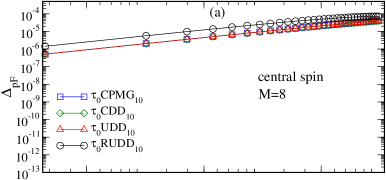
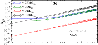
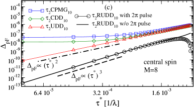
Figure 5: (Color online) Distance $\Delta_{\textrm{pF}}$ vs. the shortest pulse duration $\tau^{*}$ for various sequences at $\alpha=10$ with $T=0.09/\lambda$; the panels correspond to pulses of finite width of different order as in Fig. 3.

In panel (a) all sequences behave similarly; the dependence on $\tau^{*}$ is linear, and the RUDD behaves worst. This fact is attributed to the larger average length of the pulses. Note that in the regime depicted the distance $\Delta_{\textrm{pF}}$ is still fully dominated by the pulse errors.

In panel (b) we can nicely see the crossover from the regime where the pulse error dominates (straight lines corresponding to $(\tau^{*})^{2}$) to the saturation levels corresponding to the errors of the ideal CPMG and CDD sequence. The errors of the ideal UDD sequence is much lower so that its saturation level cannot be seen. Still the $\tau_{1}$RUDD behaves worse than the $\tau_{1}$UDD.

In panel (c) we again see the crossover from pulse errors to sequence errors on $\tau^{*}\to 0$. Interestingly, the RUDD behaves better than the UDD in that the pulse errors decrease expectedly faster $\Delta_{\text{pF,RUDD}}\propto(\tau^{*})^{3}$ compared to $\Delta_{\text{pF,UDD}}\propto(\tau^{*})^{2}$. We stress that the latter scaling is no contradiction to the pulse being second order because an error $T(\tau^{*})^{2}$ is not excluded. Fig. 5(c) establishes that such mixed terms indeed deteriorate the performance of unadapted sequences of finite-width pulses. This clarifies the behavior of RUDD relative to other sequences.

For practical implementation, it is important to point out that the behavior of $\tau_{2}$RUDD for small $\tau^{*}$ is independent of whether or not we include the very short boundary $2\pi$ pulses, cf. solid line and circles in Fig. 5(c). This is due to the shortness of these effective identity pulses.

Last but not least, we find another regime of low values of $\Delta_{\mathrm{pF}}$. This is the regime where the pulse lengths reach their maximum value because the pulses touch one another. They are back to back. Quite unexpectedly, the full RUDD including the boundary $2\pi$ pulses again permits to obtain an extremely good suppression of decoherence. This regime is very interesting because it requires only very low pulse amplitudes and a small total energy for the coherent control, cf. Eq. (10), due to the pulses of maximum length. Further studies of this relevant regime are left to future research.

Conclusions.

The analysis of sequences of finite-width pulses allows us to draw the following conclusions. They are derived from the data for the models studied, but we expect them to hold more generally.

First, the use of higher order pulses generically implies a significant improvement. Such pulses are designed such that they suppress the coupling to the bath to a high order during their action Pasini et al. (2009). Second, non-equidistant sequences such as UDD outperform or, in the worst case, perform the same as equidistant (CPMG) or concatenated (CDD) sequences.

Third, in the regime, where the pulse errors dominate the suppression of decoherence is further enhanced by varying the pulse durations along the sequence (RUDD) as suggested on analytic grounds Uhrig and Pasini (2010). This enhancement takes only place for pulses of sufficient high order. We found that it is present for second order pulses. This establishes RUDD as a promising concept and represents our central result.

Fourth, an additional interesting asset of the RUDD is that the total energy required for the coherent control by pulses increases only logarithmically with the number of pulses – in contrast to all other sequences of unvaried pulses. Hence in particular long coherence times can be realized at low energy price.

Fifth, surprisingly, we found an additional regime where the RUDD suppresses decoherence efficiently. This is the regime where the pulses are (almost) back-to-back approaching continuous modulation Gordon et al. (2008). Because in this regime the pulses reach their maximum length the required control energy is a minimum. Further research is required to study this promising regime in detail.

References

- Nielsen and Chuang (2000) M. A. Nielsen and I. L. Chuang, Quantum Computation and Quantum Information (Cambridge University Press, Cambridge, 2000).
- Haeberlen (1976) U. Haeberlen, High Resolution NMR in Solids: Selective Averaging (Academic Press, New York, 1976).
- Jenista et al. (2009) E. R. Jenista, A. M. Stokes, R. T. Branca, and W. S. Warren, J. Chem. Phys. 131, 204510 (2009).
- Gordon et al. (2008) G. Gordon, G. Kurizki, and D. A. Lidar, Phys. Rev. Lett. 101, 010403 (2008).
- Hahn (1950) E. L. Hahn, Phys. Rev. 80, 580 (1950).
- Viola and Lloyd (1998) L. Viola and S. Lloyd, Phys. Rev. A 58, 2733 (1998).
- Ban (1998) M. Ban, J. Mod. Opt. 45, 2315 (1998).
- Carr and Purcell (1954) H. Y. Carr and E. M. Purcell, Phys. Rev. 94, 630 (1954).
- Meiboom and Gill (1958) S. Meiboom and D. Gill, Rev. Sci. Inst. 29, 688 (1958).
- Uhrig (2007) G. S. Uhrig, Phys. Rev. Lett. 98, 100504 (2007); Erratum: 106, 129901 (2011a).
- Lee et al. (2008) B. Lee, W. M. Witzel, and S. Das Sarma, Phys. Rev. Lett. 100, 160505 (2008).
- Yang and Liu (2008) W. Yang and R.-B. Liu, Phys. Rev. Lett. 101, 180403 (2008).
- Biercuk et al. (2009) M. J. Biercuk, H. Uys, A. P. VanDevender, N. Shiga, W. M. Itano, and J. J. Bollinger, Nature 458, 996 (2009).
- Uys et al. (2009) H. Uys, M. J. Biercuk, and J. J. Bollinger, Phys. Rev. Lett. 103, 040501 (2009).
- Khodjasteh et al. (2011) K. Khodjasteh, T. Erdélyi, and L. Viola, Phys. Rev. A 83, 020305(R) (2011).
- Khodjasteh and Lidar (2005) K. Khodjasteh and D. A. Lidar, Phys. Rev. Lett. 95, 180501 (2005).
- Uhrig (2009) G. S. Uhrig, Phys. Rev. Lett. 102, 120502 (2009).
- West et al. (2010) J. R. West, B. H. Fong, and D. A. Lidar, Phys. Rev. Lett. 104, 130501 (2010).
- Skinner et al. (2003) T. E. Skinner, T. O. Reiss, B. Luy, N. Khaneja, and S. J. Glaser, J. Mag. Res. 163, 8 (2003).
- Viola and Knill (2003) L. Viola and E. Knill, Phys. Rev. Lett. 90, 037901 (2003).
- Sengupta and Pryadko (2005) P. Sengupta and L. P. Pryadko, Phys. Rev. Lett. 95, 037202 (2005).
- Khodjasteh and Lidar (2007) K. Khodjasteh and D. A. Lidar, Phys. Rev. A 75, 062310 (2007).
- Pryadko and Quiroz (2008) L. P. Pryadko and G. Quiroz, Phys. Rev. A 77, 012330 (2008).
- Du et al. (2009) J. Du, X. Rong, N. Zhao, Y. Wang, J. Yang, and R. B. Liu, Nature 461, 1265 (2009).
- Pasini et al. (2009) S. Pasini, P. Karbach, C. Raas, and G. S. Uhrig, Phys. Rev. A 80, 022328 (2009).
- Khodjasteh and Viola (2009) K. Khodjasteh and L. Viola, Phys. Rev. Lett. 102, 080501 (2009).
- Uhrig and Pasini (2010) G. S. Uhrig and S. Pasini, New J. Phys. 12, 045001 (2010).
- (28) No constraints are imposed on the total energy of all pulses in the sequence. We consider the bound on the amplitudes of the pulses to be the crucial experimental constraint. This is the main difference to Ref. Gordon et al. (2008) where the technique of optimum control by modulation at given total energy is developed.
- Schliemann et al. (2003) J. Schliemann, A. Khaetskii, and D. Loss, J. Phys.: Condens. Matter 15, R1809 (2003).
- Bortz and Stolze (2006) M. Bortz and J. Stolze, J. Stat. Mech. p. P06018 (2006).
- Bortz and Stolze (2007) M. Bortz and J. Stolze, Phys. Rev. B 76, 014304 (2007).
- Witzel and Das Sarma (2008) W. M. Witzel and S. Das Sarma, Phys. Rev. B 77, 165319 (2008).
- Witzel et al. (2007) W. M. Witzel, M. S. Carroll, A. Morello, L. Cywiński, and S. Das Sarma, Phys. Rev. Lett. 76, 241303 (2007).
- Cummins et al. (2003) H. K. Cummins, G. Llewellyn, and J. A. Jones, Phys. Rev. A 67, 042308 (2003).
- Khodjasteh et al. (2010) K. Khodjasteh, D. A. Lidar, and L. Viola, Phys. Rev. Lett. 104, 090501 (2010).
- Uhrig and Lidar (2010) G. S. Uhrig and D. A. Lidar, Phys. Rev. A 82, 012301 (2010).
- Lidar et al. (2008) D. Lidar, P. Zanardi, and K. Khodjasteh, Phys. Rev. A 78, 012308 (2008).
- Uhrig (2008) G. S. Uhrig, New J. Phys. 10, 083024 (2008); Corrigendum 13, 059504 (2011b).
- Cywiński et al. (2008) L. Cywiński, R. M. Lutchyn, C. P. Nave, and S. Das Sarma, Phys. Rev. B 77, 174509 (2008).
- Biercuk and Uys (2011) M. J. Biercuk and H. Uys, p. 1012.4262 (2011).
- Levitt (2005) M. H. Levitt, Spin Dynamics, Basics of Nuclear Magnetic Resonance (John Wiley & Sons, Ltd, Chichester, 2005).
- Karbach et al. (2008) P. Karbach, S. Pasini, and G. S. Uhrig, Phys. Rev. A 78, 022315 (2008).