Abstract

This paper deals with the computation of sectional curvature for the manifolds of $N$ landmarks (or feature points) in $D$ dimensions, endowed with the Riemannian metric induced by the group action of diffeomorphisms. The inverse of the metric tensor for these manifolds (i.e. the cometric), when written in coordinates, is such that each of its elements depends on at most $2D$ of the $ND$ coordinates. This makes the matrices of partial derivatives of the cometric very sparse in nature, thus suggesting solving the highly non-trivial problem of developing a formula that expresses sectional curvature in terms of the cometric and its first and second partial derivatives (we call this Mario’s formula). We apply such formula to the manifolds of landmarks and in particular we fully explore the case of geodesics on which only two points have non-zero momenta and compute the sectional curvatures of 2-planes spanned by the tangents to such geodesics. The latter example gives insight to the geometry of the full manifolds of landmarks.

1 Introduction

In the past few years there has been a growing interest, in diverse scientific communities, in modeling shape spaces as Riemannian manifolds. The study of shapes and their similarities is in fact central in computer vision and related fields (e.g. for object recognition, target detection and tracking, classification of biometric data, and automated medical diagnostics), in that it allows one to recognize and classify objects from their representation. In particular, a distance function between shapes should express the meaning of similarity between them for the application that one has in mind. One of the most mathematically sound and tractable methods for defining a distance on a manifold is to measure infinitesimal distance by a Riemannian structure and global distance by the corresponding lengths of geodesics.

Among the several ways of endowing a shape manifold with a Riemannian structure (see, for example, [17, 18, 20, 25, 28, 30]), one of the most natural is inducing it through the action of the infinite-dimensional Lie group of diffeomorphisms of the manifold ambient to the shapes being studied. You start by putting a right-invariant metric on this diffeomorphism group, as described in [27]. Then fixing a base point on the shape manifold, one gets a surjective map from the group of diffeomorphisms to the shape manifold. The right-invariance of the metric “upstairs” implies that we get a quotient metric on the shape manifold for which this map is a submersion (see below). This approach can be used to define a metric on very many shape spaces, such as the manifolds of curves [12, 26], surfaces [33], scalar images [4], vector fields [6], diffusion tensor images [5], measures [11, 13], and labeled landmarks (or “feature points”) [14, 15]. The actual geometry of these Riemannian manifolds has remained almost completely unknown until very recently, when certain fundamental questions about their curvature have started being addressed [25, 26, 32].

Among all shape manifolds, the simplest case of the manifold of landmarks in Euclidean space plays a central role. This is defined as

$$\mathcal{L}^{N}(\mathbb{R}^{D}):=\Big{\{}(P^{1},\ldots,P^{N})\,\big{|}\,P^{a}\in\mathbb{R}^{D},\;a=1,\ldots,N\Big{\}}.$$

(typically we consider landmarks $P^{a}$, $a=1,\ldots,N$ that do not coincide pairwise). It is finite-dimensional, albeit with high dimension $n=ND$, where $N$ is the number of landmarks and $D$ is the dimension of the ambient space in which they live (e.g. $D=2$ for the plane). Therefore its metric tensor may be written, in any set of coordinates, as a finite-dimensional matrix. This space is important in the study of all other shape manifolds because of a simple property of submersions: for any submersive map $f:X\rightarrow Y$, all geodesics on $Y$ lift to geodesics on $X$ and give you, in fact, all geodesics on $X$ which at one and hence all points are perpendicular to the fiber of $f$ (so called “horizontal” geodesics). This means that geodesics on the space of landmarks lift to geodesics on the diffeomorphism group and then project down to geodesics on all other shape manifolds associated to the same underlying ambient space $\mathbb{R}^{D}$. Thus geodesics of curves, surfaces, etc. in $\mathbb{R}^{D}$ can be derived from geodesics of landmark points. Technically, these are the geodesics on these shape manifolds whose momentum has finite support. This efficient way of constructing geodesics on many shape manifolds has been exploited in much recent work, e.g. [2, 8, 29].

What sort of metrics arise from submersions? Mathematically, the key point is that the inverse of the metric tensor, the inner product on the cotangent space hence called the co-metric, behaves simply in a submersion. Namely, for a submersion $f:X\rightarrow Y$, the co-metric on $Y$ is simply the restriction of the co-metric on $X$ to the pull-back 1-forms. Therefore, for the space of landmarks the cometric has a simple structure. In our case, we will see that each of its elements depends only on at most $2D$ of the $N\!D$ coordinates. Hence the matrices obtained by taking first and second partial derivatives of the cometric have a very sparse structure — that is, most of their entries are zero. This suggests that for the purpose of calculating curvature (rather than following the “classical” path of computing first and second partial derivatives of the metric tensor itself, the Christoffel symbols, et cetera) it would be convenient to write sectional curvature in terms of the inverse of the metric tensor and its derivatives. We have solved the highly non-trivial problem of developing a formula (that we call “Mario’s formula”) precisely for this purpose: for a given pair of cotangent vectors this formula expresses the corresponding sectional curvature as a function of the cometric and its first and second partial derivatives except for one term which requires the metric (but not its derivatives). This formula is closely connected to O’Neill’s formula which, for any submersion as above, connects the curvatures of $X$ and $Y$. Subtracting Mario’s formula on $X$ and $Y$ gives O’Neill’s as a corollary.

This paper deals with the problem of computing geodesics and sectional curvature for landmark spaces, and is based on results from the thesis of the first author [23]. The paper is organized as follows. We first give a few more details about the manifold of landmarks, and describe the metric induced by the action of the Lie group of diffeomorphisms. We then give a proof for the general formula expressing sectional curvature in terms of the cometric. This formula is used in the following section to compute the sectional curvature for the manifold of labeled landmarks. In the last section, we analyze the case of geodesics on which only two points have non-zero momenta and the sectional curvatures of 2-planes made up of the tangents to such geodesics. In this case, both the geodesics and the curvature are much simpler and give insight into the geometry of the full landmark space.

2 Riemannian Manifolds of Landmarks

In this section we briefly summarize how the shape space of landmarks can be given the structure of a Riemannian manifold. We refer the reader to [27, 31] for the general framework on how to endow generic shape manifolds with a Riemannian metric via the action of Lie groups of diffeomorphisms.

2.1 Mathematical preliminaries

We will first define a distance function $d:\mathcal{L}^{N}(\mathbb{R}^{D})\times\mathcal{L}^{N}(\mathbb{R}^{D})\rightarrow\mathbb{R}^{+}$ on landmark space which will then turn out to be the geodesic distance with respect to a Riemannian metric. Let $\mathcal{Q}$ be the set of differentiable landmark paths, that is:

$$\mathcal{Q}:=\Big{\{}q=(q^{1},\ldots,q^{N}):[0,1]\rightarrow\mathcal{L}^{N}(\mathbb{R}^{D})\,\Big{|}\,q^{a}\in C^{1}\big{(}[0,1],\mathbb{R}^{D}\big{)},a=1,\ldots,N\,\Big{\}}.$$

Following [31, Chapters 9, 12, 13], a Hilbert space $\big{(}V,\langle\quad,\quad\rangle_{V}\big{)}$ of vector fields on Euclidean space (which we consider as functions $\mathbb{R}^{D}\rightarrow\mathbb{R}^{D}$) is said to be admissible if (i) $V$ is continuously embedded in the space of $C^{1}$-mappings on $\mathbb{R}^{D}\to\mathbb{R}^{D}$ which are bounded together with their derivatives, (ii) $V$ is large enough: For any positive integer $M$, if $x_{1},\ldots,x_{M}\in\mathbb{R}^{D}$ and $\alpha_{1},\ldots,\alpha_{M}\in\mathbb{R}^{D}$ are such that, for all $u\in V$, $\sum_{a=1}^{M}\big{\langle}\alpha_{a},u(x_{a})\big{\rangle}_{\mathbb{R}^{D}}=0$, then $\alpha_{1}=\ldots=\alpha_{M}=0$.

The space $(V,\langle\quad,\quad\rangle_{V})$ admits a reproducing kernel: that is, for each $\alpha,x\in\mathbb{R}^{D}$ there exists $K_{x}^{\alpha}\in V$ with $\langle K_{x}^{\alpha},f\rangle_{V}=\langle\alpha,f(x)\rangle_{\mathbb{R}^{D}}$ for all $f\in V$. Further, $\langle K_{y}^{\beta},K_{x}^{\alpha}\rangle_{V}=\langle\beta,K_{x}^{\alpha}(y)\rangle_{\mathbb{R}^{D}}=\langle\alpha,K_{y}^{\beta}(x)\rangle_{\mathbb{R}^{D}}$ which is a bilinear form in $(\alpha,\beta)\in(\mathbb{R}^{D})^{2}$, thus given by a $D\times D$ matrix $K(x,y)$; the symmetry of the inner product implies that $K(y,x)=K(x,y)^{T}$ (where ^T indicates the transpose). In this paper we shall assume that $K(x,y)$ is a multiple of the identity and is translation invariant: we then write $K(x,y)$ simply as $K(x-y)\,\mathbb{I}_{D}$ (where $\mathbb{I}_{D}$ is the $D\times D$ identity matrix); the scalar reproducing kernel $K:\mathbb{R}^{D}\rightarrow\mathbb{R}$ must be symmetric, and positive definite (see [31, §9.1] for details).

There are other very natural admissible norms on vector fields $v$ whose kernels are not multiples of the identity, e.g. one can add a multiple of $\operatorname{div}(v)^{2}$ to any norm and then $K$ will intertwine different components of $v$. The most natural examples of the norms we will consider are given by inner products

$$\langle u,v\rangle_{V}=\langle u,v\rangle_{L}:=\int_{\mathbb{R}^{D}}\big{\langle}Lu(x),v(x)\big{\rangle}_{\mathbb{R}^{D}}\ dx,$$ (1)

where $L$ is a self-adjoint elliptic scalar differential operator of order greater than $D+2$ with constant coefficients which is applied separately to each of the scalar components of the vector field $u=(u^{1},\ldots,u^{D})$. By the Sobolev embedding theorem then $V$ consists of $C^{1}$-functions on $\mathbb{R}^{D}$ which are bounded together with their derivatives. If $K$ is a scalar fundamental solution (or Green’s function [9]) so that $L(K)(x)=\delta(x)$, then the reproducing kernel is given by $K_{x}^{\alpha}=K(\quad-x)\,\alpha$. A possible choice of the operator is $L=(1-A^{2}\Delta)^{k}$ (where $A\in\mathbb{R}$ is a scaling factor, $k\in\mathbb{N}$ and $\Delta$ is the Laplacian operator), with $k>\frac{D}{2}+1$, in which case (1) becomes the Sobolev norm:

$$\|u\|_{L}^{2}=\int_{\mathbb{R}^{D}}\sum_{\ell=1}^{D}\sum_{m=0}^{k}\binom{k}{m}A^{2m}\sum_{|\alpha|=m}\big{|}D^{\alpha}u^{\ell}\big{|}^{2}\ dx,$$ (2)

When $L=(1-A^{2}\Delta)^{k}$ the scalar kernel $K$ has the form $K(x-y)=\gamma\big{(}\|x-y\|_{\mathbb{R}^{D}}\big{)}$, with:

$$\gamma(\varrho)=\frac{1}{2^{k+\frac{D}{2}-1}\pi^{\frac{D}{2}}\,\Gamma(k)\,A^{D}}\Big{(}\frac{\varrho}{A}\Big{)}^{k-\frac{D}{2}}\,K_{k-\frac{D}{2}}\!\big{(}\frac{\varrho}{A}\big{)},\quad\varrho>0,$$ (3)

where $K_{\nu}$ (with $\nu=k-\frac{D}{2}$) is a modified Bessel function [1] of order $\nu$ (not to be confused with the symbol $K$ we use for the kernel of $V$).

In summary, the scalar kernels that we consider in this paper will always have the properties:

(K1) $K$ is positive definite;

(K2) $K$ is symmetric, i.e. $K(x)=K(-x)$, $x\in\mathbb{R}^{D}$.

In addition, in certain sections we will introduce the following simplifying assumptions:

(K3) $K$ is twice continuously differentiable, $K\in C^{2}(\mathbb{R}^{D})$;

(K4) $K$ is rotationally invariant, i.e. $K(x)=\gamma(\|x\|_{\mathbb{R}^{D}})$, $x\in\mathbb{R}^{D}$, for some $\gamma\in C^{2}\big{(}[0,\infty)\big{)}$.

Note that if (K4) holds then $\gamma(0)\geq|\gamma(\rho)|$ for all $\rho\geq 0$ by (K1) and (K2). Also, the bell-shaped Bessel kernels of the type (3) satisfy all of the above when $k>\frac{D}{2}+1$.

Now fix any admissible Hilbert space of vector fields. The space $L^{p}([0,1],V)$ is the set of functions $v:[0,1]\rightarrow V$ such that:

$$\|v\|_{L^{p}([0,1],V)}:=\Big{(}\int_{0}^{1}\|v(t,\;\;\;)\|^{p}_{V}\ dt\Big{)}^{\frac{1}{p}}<\infty.$$

The space $L^{2}([0,1],V)$ is a subset of $L^{1}([0,1],V)$ and is in fact a Hilbert space with inner product $\langle u,v\rangle_{L^{2}([0,1],V)}:=\int_{0}^{1}\langle u,v\rangle_{V}\ dt$. It is well known from the theory of ordinary differential equations [7] that for any $v\in L^{1}([0,1],V)$, the $D$-dimensional non-autonomous dynamical system $\dot{z}=v_{t}(z)$, with initial condition $z(t_{0})=x$, has a unique solution of the type $z(t)=\psi(t,t_{0},x)$. Let $\varphi_{st}^{v}(x):=\psi(t,s,x)$; fixing $t=1$ and $s=0$ we get $\varphi^{v}:=\varphi_{01}^{v}$, which is the diffeomorphism generated by $v$. For an admissible Hilbert space we will call the set

$$\mathcal{G}_{V}:=\big{\{}\varphi^{v}:v\in L^{1}\big{(}[0,1],V\big{)}\big{\}}$$

the group of diffeomorphisms generated by $V$; by [31, Chapter 12] it is a metric space and a topological group. But, in the language of manifolds, $\mathcal{G}_{V}$ is not an infinite-dimensional Lie group [19]. $V$ is not a Lie algebra, but is the completion of the Lie algebra of $C^{\infty}$-vector fields with compact support with respect to $\|\quad\|_{V}$.

2.2 Definition of the distance function

For velocity vector fields $v\in L^{2}([0,1],V)$ and landmark trajectories $q\in\mathcal{Q}$ define the energy

$$E_{\lambda}[v,q]\equiv E[v,q]:=\int_{0}^{1}\Big{(}\big{\|}v(t,\quad)\big{\|}_{V}^{2}+\lambda\sum_{a=1}^{N}\Big{\|}\frac{dq^{a}}{dt}(t)-v\big{(}t,q^{a}(t)\big{)}\Big{\|}_{\mathbb{R}^{D}}^{2}\Big{)}\ dt,$$ (4)

where $\lambda\in(0,\infty]$ is a fixed smoothing parameter (soon to be described). We claim that a distance function $d$ on $\mathcal{L}^{N}(\mathbb{R}^{D})$ between two landmark sets (or shapes) $I=(x^{1},x^{2},\ldots,x^{N})$ and $I^{\prime}=(y^{1},y^{2},\ldots,y^{N})$ can be defined as

$$d(I,I^{\prime}):=\inf_{v,q}\Big{\{}\sqrt{E[v,q]}:v\in L^{2}\big{(}[0,1],V\big{)},\,q\in\mathcal{Q}\mbox{ with }q(0)=I,\,q(1)=I^{\prime}\Big{\}};$$ (5)

in the next subsection we will argue that the above function is in fact a geodesic distance with respect to a Riemannian metric. We treat the minimization of (4) as our starting point; it is the “energy of a metamorphosis” as formulated in [31, Chapter 13].

The above infimum is computed over all differentiable landmark paths $q\in\mathcal{Q}$ that satisfy the boundary conditions ($q^{a}(0)=x^{a}$ and $q^{a}(1)=y^{a}$, $a=1,\ldots,N$), and vector fields $v\in L^{2}([0,1],V)$. The resulting landmark trajectories $\{q^{a}(t),t\in[0,1]\}_{a=1,\ldots,N}$ follow the minimizing velocity field more or less exactly, depending on the value of the smoothing parameter $\lambda\in(0,\infty]$; it is a weight between the first term, that measures the smoothness of the vector field that generates the diffeomorphism, and the second term, that measures how closely the landmark trajectories actually follow the vector field.

The exact matching problem is the following: given two sets of landmarks $I=(x^{1},x^{2},\ldots,x^{N})$ and $I^{\prime}=(y^{1},y^{2},\ldots,y^{N})$ with $x^{a}\not=x^{b}$ and $y^{a}\not=y^{b}$ for any $a\not=b$, minimize the energy

$$E_{\infty}[v]:=\int_{0}^{1}\|v(t,\quad)\|_{V}^{2}\,dt$$

among all $v\in L^{2}([0,1],V)$ such that $\varphi^{v}(x^{a})=y^{a}$, $a=1,\ldots,N$. In this case the landmark trajectories are defined as the solutions to the ordinary differential equations $\dot{q}^{a}=v(t,q^{a})$, $a=1,\ldots,N$. Note that this is equivalent to solving (4) for $\lambda=\infty$, since such equations are obtained by setting the integrands of the second term in the right-hand side of (4) equal to zero. When $\lambda<\infty$ in (4) we have regularized matching, i.e. the landmark trajectories “almost” satisfy such set of ordinary differential equations; this allows for the time varying vector field to be smoother. For this reason the second term in the right-hand side of (4) is often referred to as smoothing term; by allowing smoother vector fields the distance $d$ is made tolerant to small diffeomorphisms and therefore more robust to object variations due to noise in the data.

2.3 Minimizing velocity fields and Riemannian formulation

By manipulating expression (4) we will now show that it is equivalent to the energy of a path $q\in\mathcal{Q}$ with respect to a Riemannian metric.

Notation.

Consider a landmark $q=(q^{1},\ldots,q^{N})$ in $\mathcal{L}^{N}(\mathbb{R}^{D})$. The $D$ scalar components in Euclidean coordinates of the $N$ landmark trajectories $q^{a}=(q^{a1},\ldots,q^{aD})$, $a=1,\ldots,N$ can be ordered either into an $N\times D$ matrix or in a tall concatenated column vector. We shall always use indices $a,b,c,\ldots\in\{1,\dots,N\}$ as landmark indices, and $i,j,k,\ldots\in\{1,\dots,D\}$ as space coordinates in $\mathbb{R}^{D}$. We will associate to each of the $N$ landmarks $q^{a}\in\mathbb{R}^{1\times D}$ a momentum $p_{a}\in\mathbb{R}^{1\times D}$ (defined in the next proposition) which we will write, in coordinates, as $p_{a}=(p_{a1},\ldots,p_{aD})$, for each $a=1,\ldots,N$. The components of momenta can also be ordered into an $N\times D$ matrix or in a long row vector. We chose superscript indices for landmark coordinates and subscript indices for momenta.

For a given set of landmarks $(q^{1},\ldots,q^{N})\in\mathcal{L}^{N}(\mathbb{R}^{D})$ we will define the symmetric $N\times N$ matrix $\mathbf{K}(q):=\bigl{(}K(q^{a}-q^{b})\bigr{)}_{a,b=1,\dots,N}$. The matrix $\mathbf{K}(q)$ is positive definite by property (K1) of the kernel.

Proposition 1.

For a fixed landmark path $\overline{q}=\big{\{}\overline{q}^{a}:[0,1]\rightarrow\mathbb{R}^{D}\big{\}}_{a=1}^{N}\in\mathcal{Q}$ there exists a unique minimizer with respect to $v\in L^{2}([0,1],V)$ of the energy $E[v,\overline{q}]$, namely:

$$v^{\ast}(t,x):=\sum_{a=1}^{N}p_{a}(t)\,K\big{(}x-\overline{q}^{a}(t)\big{)},\qquad t\in[0,1],\;x\in\mathbb{R}^{D},$$ (6)

where the components of the momenta are given by:

$$p_{ai}(t)=\sum_{b=1}^{N}\Big{(}\mathbf{K}\big{(}\overline{q}(t)\big{)}+\frac{\mathbb{I}_{N}}{\lambda}\Big{)}^{-1}_{ab}\cdot\frac{d}{dt}\overline{q}^{bi}(t),\qquad t\in[0,1],$$ (7)

$a=1,\ldots,N$, $i=1,\ldots,D$ (here $\mathbb{I}_{N}$ indicates the $N\times N$ identity matrix).

Remark.

What the above proposition essentially says is that the vector field of minimum energy that transports the $N$ landmarks along fixed trajectories is, at any point of time, the linear combination of $N$ lumps of velocity, each centered at a landmark point. The directions and amplitudes of the summands are determined precisely by the momenta.

Proof of Proposition 1.

Using property (ii) of the admissible Hilbert space $V$, [31, Lemma 9.5] shows that for given $q=(q^{1},\dots,q^{N})\in\mathcal{L}^{N}(\mathbb{R}^{D})$ we have the orthogonal decomposition

$$V=\big{\{}v\in V:v(q^{a})=0,a=1,\dots N\big{\}}\oplus\big{\{}v=\textstyle\sum_{a=1}^{N}\alpha_{a}K(\quad-q^{a}):\alpha_{a}\in\mathbb{R}^{D}\big{\}}.$$ (8)

Thus the minimizer must have the form

$$v(t,x)=\sum_{a=1}^{N}\alpha_{a}(t)\,K\big{(}x-\overline{q}^{a}(t)\big{)},\qquad t\in[0,1],\;x\in\mathbb{R}^{D},$$ (9)

for some coefficients $\alpha_{a}\in C([0,1],\mathbb{R}^{D})$, $a=1,\ldots,N$, to be computed. For velocities of the type (9) the energy (4) can be rewritten as

$$E[v,\overline{q}]=\int_{0}^{1}\sum_{i=1}^{D}\sum_{a,b=1}^{N}\Big{\{}\alpha_{ai}K(\overline{q}^{a}-\overline{q}^{b})\alpha_{bi}+\lambda\,\big{|}\alpha_{ai}K(\overline{q}^{a}-\overline{q}^{b})-\dot{\overline{q}}^{bi}\big{|}^{2}\Big{\}}\ dt.$$ (10)

Setting the first variation of (10) with respect to coefficients $\alpha_{ai}$ to zero yields the momenta (7). ∎

It is convenient, at this point, to introduce the $ND\times ND$, block-diagonal matrix

$$g(q):=\begin{pmatrix}\big{(}\mathbf{K}(q)+\frac{\mathbb{I}_{N}}{\lambda}\big{)}^{-1}&0&\cdots&0\\ 0&\big{(}\mathbf{K}(q)+\frac{\mathbb{I}_{N}}{\lambda}\big{)}^{-1}&\cdots&0\\ \vdots&\vdots&\ddots&\vdots\\ 0&0&\cdots&\big{(}\mathbf{K}(q)+\frac{\mathbb{I}_{N}}{\lambda}\big{)}^{-1}\end{pmatrix},$$ (11)

where the $N\times N$ block $\big{(}\mathbf{K}(q)+\frac{\mathbb{I}_{N}}{\lambda}\big{)}^{-1}$ is repeated $D$ times; the choice of symbol $g$ is justified by the fact that (11) is, as we shall see soon, precisely the Riemannian metric tensor with which we are endowing the manifold of landmarks, written in coordinates.

Thus for a fixed path $\overline{q}\in\mathcal{Q}$ the minimizer of $E[v,\overline{q}]$ with respect to $v\in L^{2}([0,1],V)$ is given by (6); since it depends on $\overline{q}$ we will write it, with an abuse of notation, as $v^{\ast}(\overline{q})$. We can define

$$\widetilde{E}[\overline{q}]:=E[v^{\ast}(\overline{q}),\overline{q}],$$ (12)

which depends only on the arbitrary path $\overline{q}\in\mathcal{Q}$. The energy (12) is “equivalent” to the energy $E[v,q]$, in that:

(a) if $(\hat{v},\hat{q})$ minimizes $E[v,q]$ then $\hat{q}$ minimizes $\widetilde{E}[q]$, and $E[\hat{v},\hat{q}]=\widetilde{E}[\hat{q}]$;

(b) if $\hat{q}$ minimizes $\widetilde{E}[q]$ then $(v^{\ast}(\hat{q}),\hat{q})$ minimizes $E[v,q]$, and $E[v^{\ast}(\hat{q}),\hat{q}\,]=\widetilde{E}[\hat{q}\,]$.

Proposition 2.

For an arbitrary landmark trajectory $q\in\mathcal{Q}$ the energy $\widetilde{E}[q]$ is given by:

$$\widetilde{E}[q]=\int_{0}^{1}\dot{q}(t)^{T}g\big{(}q(t)\big{)}\,\dot{q}(t)\,dt=\int_{0}^{1}\sum_{a,b=1}^{N}\sum_{i=1}^{D}\dot{q}^{ai}(t)\,\dot{q}^{bi}(t)\Big{(}\mathbf{K}\big{(}q\big{(}t))+\frac{\mathbb{I}_{N}}{\lambda}\Big{)}^{-1}_{ab}\,dt$$ (13)

In the above equation $\dot{q}(t)$ is intended as an $ND$-dimensional column vector obtained by stacking the column vectors $(\dot{q}^{1i}(t),\ldots,\dot{q}^{Ni}(t))^{T}$, $i=1,\ldots,D$ (again, the superscript ^T indicates the transpose of a vector).

Proof.

Following definition (12), formulae (7) for the momenta are inserted into the modified expression (10) for energy $E[v,q]$. Simple matrix manipulations finally yield the right-hand side of (13). ∎

Remarks.

Expression (13) has exactly the form of the energy of a path $q$ with respect to Riemannian metric tensor (11). Whence given two landmark configurations $I$ and $I^{\prime}$ in $\mathcal{L}^{N}(\mathbb{R}^{D})$ we have that if $\hat{q}$ minimizes (13) among all paths in $q\in\mathcal{Q}$ such that $q(0)=I$ and $q(1)=I^{\prime}$ then $(\widetilde{E}[\hat{q}])^{1/2}$ is the geodesic distance between $I$ and $I^{\prime}$. By point (b) above we also have that $(v^{\ast}(\hat{q}),\hat{q})$ is a minimum of energy $E[v,q]$, so $d(I,I^{\prime})$ defined in (5) coincides with $(\widetilde{E}[\hat{q}])^{1/2}$ and is the geodesic distance between $I$ and $I^{\prime}$ with respect to the metric tensor $g$.

The Lagrangian function that corresponds to the energy (13) is:

$$\mathcal{L}(q,\dot{q})=\frac{1}{2}\,\dot{q}^{T}g(q)\dot{q}=\frac{1}{2}\sum_{a,b=1}^{N}\sum_{i=1}^{D}\dot{q}^{ai}\dot{q}^{bi}\Big{(}\mathbf{K}(q)+\frac{\mathbb{I}_{N}}{\lambda}\Big{)}^{-1}_{ab}.$$ (14)

In Hamiltonian mechanics [3, p. 60] the “momenta” are defined as $p_{ai}=\partial\mathcal{L}/\partial\dot{q}^{ai}$, or, in vector notation, $p_{(i)}=\partial\mathcal{L}/\partial\dot{q}^{(i)}$ (for $i=1,\ldots,D$). Applying such definition to (14) yields precisely equations (7) of Proposition 1. Whence the use of the term momenta is justified.

Note that for small values of the parameter $\lambda$ the metric tensor $g$, written in coordinates, gets close (up to a multiplicative constant) to the $ND\times ND$ identity matrix; in other words, for $\lambda\rightarrow 0$, $g$ converges to a Euclidean metric and the geodesic curves become straight lines. On the other hand, for $\lambda\rightarrow\infty$ (exact matching) the metric converges to $[\mathrm{diag}\{\mathbf{K}(q),\ldots,\mathbf{K}(q)\}]^{-1}$ (block $\mathbf{K}(q)$ is repeated $D$ times). In general, the block-diagonal form of the metric tensor $g$ given by (11) follows from the fact that the operator $L$ in (2) is applied separately to each of the components of the velocity field; however the dynamics of the $D$ dimensions of $q$ are not decoupled since all $N\!D$ components of $q$ appear in each diagonal block of $g$.

In the case of exact matching landmarks “never collide” (their trajectories are precisely defined by diffeomorphisms of $\mathbb{R}^{D}$): it takes an infinite amount of energy to make any two landmarks coincide. So under the condition $\lambda=\infty$ the manifold of landmarks can actually be taken as the set:

$$\mathcal{L}^{N}(\mathbb{R}^{D})=\Big{\{}(P^{1},\ldots,P^{N})\,\big{|}\,P^{a}\in\mathbb{R}^{D},P^{a}\not=P^{b}\mbox{ if }a\not=b\Big{\}}.$$ (15)

Figure 1 shows the qualitative behavior of geodesics in $\mathcal{L}^{2}(\mathbb{R}^{2})$, with $\lambda=\infty$. In the case illustrated on the left-hand side both landmarks travel in the same direction (from left to right, as indicated by the arrows): the two arcs of the geodesic “attract” each other, or in other words the two landmarks tend to “carpool” by using a velocity field with the smallest possible support so to minimize the $L^{2}$ part (i.e. the first term) of the Sobolev norm (2) of the velocity field. On the other hand when the two landmarks travel in opposite directions (as illustrated on the right-hand side of Figure 1) they try to avoid each other so that the higher order terms of the Sobolev norm are kept small; we shall return on the issue of obstacle avoidance at the end of this paper. A typical geodesic in $\mathcal{L}^{4}(\mathbb{R}^{2})$ (again with $\lambda=\infty$) is shown in Figure 2.

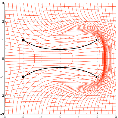
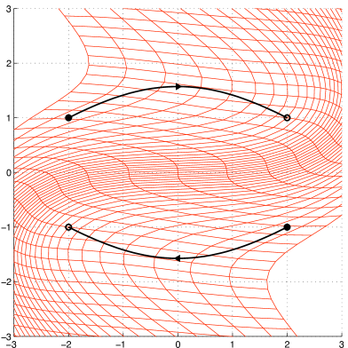
Figure 1: Two trajectories in $\mathcal{L}^{2}(\mathbb{R}^{2})$. Bullets $(\bullet)$ and circles $(\circ)$ are the initial and final sets of landmarks, respectively. The grids represents the two corresponding diffeomorphisms $\varphi_{01}^{v}$.

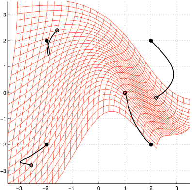
Figure 2: A typical geodesic trajectory in $\mathcal{L}^{4}(\mathbb{R}^{2})$. Bullets $(\bullet)$ and circles $(\circ)$ are the initial and final sets of landmarks, respectively. The grid represents the corresponding diffeomorphism $\varphi_{01}^{v}$.

Conclusion.

We have shown that distance $d(I,I^{\prime})$, $I,I^{\prime}\in\mathcal{L}^{N}(\mathbb{R}^{D})$ defined in (5) is in fact the geodesic distance with respect to a Riemannian metric. In coordinates, the corresponding Riemannian metric tensor is given by (11), which is such that each element of its inverse (the cometric) depends on at most $2D$ of the $N\!D$ coordinates. Whence the first and second partial derivatives of the cometric have a very sparse structure. This gives us motivation for deriving a general formula for computing sectional curvature in terms of the cometric and its derivatives in lieu of the metric and its derivatives, which will be done in the next section.

3 Sectional Curvature in terms of the Cometric

3.1 Generalities and notation on sectional curvature

Let $\mathcal{M}$ be an $n$-dimensional Riemannian manifold. If we consider a local chart $(U,\varphi)$ on the manifold with coordinates $(x^{1},\ldots,x^{n})$, we have the induced 1-forms $dx^{1},\dots,dx^{n}$ and coordinate vector fields $\{\partial_{1}:=\frac{\partial}{\partial x^{1}},\ldots,\partial_{n}=\frac{\partial}{\partial x^{n}}\}$. The metric tensor $g:T\mathcal{M}\times_{\mathcal{M}}T\mathcal{M}\rightarrow\mathbb{R}$ can be represented as $g|_{U}=g(\partial_{i},\partial_{j})\,dx^{i}\otimes dx^{j}=:g_{ij}\,dx^{i}\otimes dx^{j}$ (here, as in the rest of the current section, we are using Einstein’s summation convention). For each $p\in\mathcal{M}$ we get a positive definite matrix with elements $g_{ij}(p)=g_{p}(\partial_{i},\partial_{j})$. With an abuse of notation we will write $g_{ij}(x)$ instead of $(g_{ij}\circ\varphi^{-1})(x)$, $x\in\varphi(U)\subset\mathbb{R}^{n}$.

Notation.

We shall denote the partial derivatives of the elements of the metric tensor $g$ as $g_{ij,k}(x):=\,\frac{\partial}{\partial x^{k}}g_{ij}(x)=\partial_{k}g_{ij}$ and $g_{ij,k\ell}(x):=\frac{\partial^{2}}{\partial x^{\ell}\partial x^{k}}\,g_{ij}(x)=\partial_{\ell}\partial_{k}g_{ij}$. Also, we will indicate the cometric as $g^{-1}|_{U}=g^{ij}\partial_{i}\otimes\partial_{j}$ (so that $g^{ij}g_{jk}=\delta^{i}_{k}$) and their partial derivatives with $g^{ij}_{{\color[rgb]{1,1,1}ij},k\ }\!\!(x):=\,\frac{\partial}{\partial x^{k}}g^{ij}(x)$ and $g^{ij}_{{\color[rgb]{1,1,1}ij},k\ell\ }\!\!(x):=\frac{\partial^{2}}{\partial x^{\ell}\partial x^{k}}\,g^{ij}(x)$.

For a tangent vectors $X=X^{i}\partial_{i}$ we consider the 1-form $X^{\flat}:=X^{i}g_{ij}dx^{j}=:X_{j}dx^{j}$ (indices lowered), and for a 1-form $\alpha=\alpha_{i}dx^{i}$ we have the tangent vector $\alpha^{\sharp}:=\alpha_{i}g^{ij}\partial_{j}$ (indices lifted).

Indicating with $\mathcal{X}(\mathcal{M})$ the space of smooth vector fields on the manifold $\mathcal{M}$, let $\nabla:\mathcal{X}(\mathcal{M})\times\mathcal{X}(\mathcal{M})\rightarrow\mathcal{X}(\mathcal{M})$ be the Levi-Civita connection [16, 21] of the Riemannian manifold. The Christoffel symbols $\Gamma_{ij}^{k}$ are defined by $\nabla_{\partial_{i}}\partial_{j}=\Gamma_{ij}^{k}\partial_{k}$, and it is well known that they have the form: $\Gamma_{ij}^{k}=\frac{1}{2}g^{k\ell}(g_{i\ell,j}+g_{j\ell,i}-g_{ij,\ell})$. The Riemannian curvature endomorphism is the map $R:\mathcal{X}(\mathcal{M})\times\mathcal{X}(\mathcal{M})\times\mathcal{X}(\mathcal{M})\rightarrow\mathcal{X}(\mathcal{M})$ given by $R(X,Y)Z=\nabla_{X}\nabla_{Y}Z-\nabla_{Y}\nabla_{X}Z-\nabla_{[X,Y]}Z.$ In local coordinates $R(\partial_{i},\partial_{j})\partial_{k}=R_{ijk}^{\ell}\partial_{\ell}$, and $R_{ijkm}:=\langle R(\partial_{i},\partial_{j})\partial_{k},\partial_{m}\rangle_{g}=g_{m\ell}R_{ijk}^{\ell}.$ The Riemannian curvature tensor acts on vector fields as follows:

$$R(X,Y,Z,W):=\langle R(X,Y)Z,W\rangle_{g}$$ (16)

and in coordinates it is written as $R=R_{ijkm}dx^{i}\otimes dx^{j}\otimes dx^{k}\otimes dx^{m}$. The Riemannian curvature tensor has a number of symmetries: (i) $R_{ijk\ell}=-R_{jik\ell}$; (ii) $R_{ijk\ell}=-R_{ij\ell k}$; (iii) $R_{ijk\ell}=R_{k\ell ij}$; and (iv) $R_{ijk\ell}+R_{jki\ell}+R_{kij\ell}=0$ (first Bianchi identity). With such conventions, the sectional curvature associated to a pair of non-parallel tangent vectors $X$ and $Y$ is computed by:

$$\mathcal{K}(X,Y)\;\,=\;\,\frac{R(X,Y,Y,X)}{\|X\|_{g}^{2}\|Y\|_{g}^{2}-\langle X,Y\rangle_{g}^{2}}\;\,=\;\,\frac{R_{ijkm}X^{i}Y^{j}Y^{k}X^{m}}{\|X\|_{g}^{2}\|Y\|_{g}^{2}-\langle X,Y\rangle_{g}^{2}}\,.$$ (17)

In order to express the numerator of sectional curvature (17) in terms of the elements of the cometric and its derivatives (i.e. $g^{ij}$, $g^{ij}_{{\color[rgb]{1,1,1}ij},k\ }\!$, and $g^{ij}_{{\color[rgb]{1,1,1}ij},k\ell\ }\!\!$) we consider the covariant expression of the Riemannian curvature tensor:

$$R^{ursv}:=R_{ijkm}\,g^{iu}g^{jr}g^{ks}g^{mv},$$ (18)

which we call the dual Riemannian curvature tensor. Similarly we consider the covariant or dual Christoffel symbols

$$\Gamma_{u}^{rs}:=g^{ir}g^{js}g_{ku}\Gamma^{k}_{ij}\,,$$ (19)

which are symmetric in the indices $r$ and $s$.

To achieve notational compactness we will use the following symbols:

$$g^{ij,k}:=g^{ij}_{{\color[rgb]{1,1,1}ij},\xi\ }g^{\xi k}\;\;\mbox{ and }\;\;g^{ij,k\ell}:=g^{ij}_{{\color[rgb]{1,1,1}ij},\xi\eta\ }g^{\xi k}g^{\eta\ell};$$ (20)

Using that $g=Q^{-1}$ implies $\partial_{k}g=-Q^{-1}\cdot\,\partial_{k}Q\cdot Q^{-1}$ one immediately sees that

$$\Gamma_{u}^{rs}=-\frac{1}{2}\,g_{u\varphi}\big{(}g^{s\varphi,r}+g^{r\varphi,s}-g^{rs,\varphi}\big{)}.$$

Proposition 3.

The following expression holds for the Riemannian curvature tensor:

$$2R_{ijkm}=g_{ik,jm}+g_{jm,ik}-g_{jk,im}-g_{im,jk}+2\Gamma^{\alpha}_{ik}\Gamma^{\beta}_{jm}g_{\alpha\beta}-2\Gamma^{\alpha}_{jk}\Gamma^{\beta}_{im}g_{\alpha\beta}.$$ (21)

For a proof see [24, §24.9].

3.2 Mario’s formula

Proposition 4.

The following expression holds for the dual Riemannian curvature tensor:

$$2R^{ursv}= -g^{us,rv}-g^{rv,us}+g^{rs,uv}+g^{uv,rs}+2\Gamma_{\rho}^{rv}\Gamma_{\sigma}^{us}g^{\rho\sigma}-2\Gamma_{\rho}^{rs}\Gamma_{\sigma}^{uv}g^{\rho\sigma}$$

$$+\;\,g^{r\lambda,u}g_{\lambda\mu}\,g^{\mu v,s}-g^{r\lambda,u}g_{\lambda\mu}\,g^{\mu s,v}+g^{u\lambda,r}g_{\lambda\mu}\,g^{\mu s,v}-g^{u\lambda,r}g_{\lambda\mu}\,g^{\mu v,s}$$ (22)

$$+\;\,g^{r\lambda,s}g_{\lambda\mu}\,g^{\mu v,u}+g^{u\lambda,v}g_{\lambda\mu}\,g^{\mu s,r}-g^{r\lambda,v}g_{\lambda\mu}\,g^{\mu s,u}-g^{u\lambda,s}g_{\lambda\mu}\,g^{\mu v,r}.$$

Proof.

We will manipulate (21) and write it in the form $R_{ijkm}=g_{iu}g_{jr}g_{ks}g_{mv}R^{ursv}$ by factoring $g_{iu}g_{jr}g_{ks}g_{mv}$ out of each term; what will be left will be precisely the expression for $R^{ursv}$.

The terms in (21) involving Christoffel symbols are, by (19):

$$\Gamma^{\alpha}_{ik}\Gamma^{\beta}_{jm}g_{\alpha\beta}=g_{iu}g_{ks}g^{\alpha\sigma}\,\Gamma^{us}_{\sigma}\,g_{jr}g_{mv}g^{\rho\beta}\,\Gamma^{rv}_{\rho}\,g_{\alpha\beta} =g_{iu}g_{jr}g_{ks}g_{mv}\big{(}\Gamma^{rv}_{\rho}\Gamma^{us}_{\sigma}g^{\rho\sigma}\big{)},$$ (23)

$$\mbox{and similarly: }\;\;\;\;\;\;\;\;\;\;\;\;\;\;\;\;\Gamma^{\alpha}_{jk}\Gamma^{\beta}_{im}g_{\alpha\beta} =g_{iu}g_{jr}g_{ks}g_{mv}\big{(}\Gamma^{rs}_{\rho}\Gamma^{uv}_{\sigma}g^{\rho\sigma}\big{)}.$$ (24)

As we noted before, if $g=Q^{-1}$ then $\partial_{j}g=-Q^{-1}\cdot\,\partial_{j}Q\cdot Q^{-1}$ and similarly it is the case that $\partial_{m}\partial_{j}g=Q^{-1}\cdot\big{(}\partial_{m}Q\cdot Q^{-1}\cdot\partial_{j}Q+\partial_{j}Q\cdot Q^{-1}\cdot\partial_{m}Q-\partial_{m}\partial_{j}Q\big{)}\cdot Q^{-1},$ i.e., in index notation,

$$g_{ik,jm} =g_{iu}\big{(}g^{u\lambda}_{{\color[rgb]{1,1,1}u\lambda},m\ }g_{\lambda\mu}\,g^{\mu s}_{{\color[rgb]{1,1,1}\mu s},j\ }+g^{u\lambda}_{{\color[rgb]{1,1,1}u\lambda},j\ }g_{\lambda\mu}\,g^{\mu s}_{{\color[rgb]{1,1,1}\mu s},m\ }-g^{us}_{{\color[rgb]{1,1,1}us},jm\ }\!\!\big{)}g_{sk}\,$$

$$=g_{iu}g_{ks}\delta^{\xi}_{j}\delta^{\eta}_{m}\big{(}g^{u\lambda}_{{\color[rgb]{1,1,1}u\lambda},\eta\ }g_{\lambda\mu}\,g^{\mu s}_{{\color[rgb]{1,1,1}\mu s},\xi\ }+g^{u\lambda}_{{\color[rgb]{1,1,1}u\lambda},\xi\ }g_{\lambda\mu}\,g^{\mu s}_{{\color[rgb]{1,1,1}\mu s},\eta\ }-g^{us}_{{\color[rgb]{1,1,1}us},\xi\eta\ }\!\!\big{)}$$

$$=g_{iu}g_{ks}g_{jr}g_{mv}\big{[}g^{r\xi}g^{v\eta}\big{(}g^{u\lambda}_{{\color[rgb]{1,1,1}u\lambda},\eta\ }g_{\lambda\mu}\,g^{\mu s}_{{\color[rgb]{1,1,1}\mu s},\xi\ }+g^{u\lambda}_{{\color[rgb]{1,1,1}u\lambda},\xi\ }g_{\lambda\mu}\,g^{\mu s}_{{\color[rgb]{1,1,1}\mu s},\eta\ }-g^{us}_{{\color[rgb]{1,1,1}us},\xi\eta\ }\!\!\big{)}\big{]}$$

$$=g_{iu}g_{jr}g_{ks}g_{mv}\big{(}g^{u\lambda,v}g_{\lambda\mu}\,g^{\mu s,r}+g^{u\lambda,r}g_{\lambda\mu}\,g^{\mu s,v}-g^{us,rv}\big{)},$$ (25)

where we have used definitions (20). Similarly, we can achieve the factorizations:

$$g_{jm,ik} =g_{iu}g_{jr}g_{ks}g_{mv}\,\big{(}g^{r\lambda,u}g_{\lambda\mu}\,g^{\mu v,s}+g^{r\lambda,s}g_{\lambda\mu}\,g^{\mu v,u}-g^{rv,us}\big{)},$$ (26)

$$-g_{jk,im} =g_{iu}g_{jr}g_{ks}g_{mv}\,\big{(}-g^{r\lambda,u}g_{\lambda\mu}\,g^{\mu s,v}-g^{r\lambda,v}g_{\lambda\mu}\,g^{\mu s,u}+g^{rs,uv}\big{)},$$ (27)

$$-g_{im,jk} =g_{iu}g_{jr}g_{ks}g_{mv}\,\big{(}-g^{u\lambda,r}g_{\lambda\mu}\,g^{\mu v,s}-g^{u\lambda,s}g_{\lambda\mu}\,g^{\mu v,r}+g^{uv,rs}\big{)}.$$ (28)

Inserting (23)$\div$(28) into (21) we can write $R_{ijkm}=g_{iu}g_{jr}g_{ks}g_{mv}R^{ursv}$, with $R^{ursv}$ given by (22). ∎

Proposition 5.

The dual Riemannian curvature tensor may also be written as follows:

$$2R^{ursv}= -g^{us,rv}-g^{rv,us}+g^{rs,uv}+g^{uv,rs}$$ (T₁)

$$-\frac{1}{2}\big{\{}g^{rs}_{{\color[rgb]{1,1,1}rs},\rho\ }g^{\rho\sigma}g^{uv}_{{\color[rgb]{1,1,1}uv},\sigma\ }\!\!-g^{rs}_{{\color[rgb]{1,1,1}rs},\rho\ }\!\big{(}g^{\rho u,v}+g^{\rho v,u}\big{)}-g^{uv}_{{\color[rgb]{1,1,1}uv},\sigma\ }\!\big{(}g^{\sigma r,s}+g^{\sigma s,r}\big{)}\big{\}}$$ (T₂)

$$+\frac{1}{2}\big{\{}g^{rv}_{{\color[rgb]{1,1,1}rv},\rho\ }g^{\rho\sigma}g^{us}_{{\color[rgb]{1,1,1}us},\sigma\ }\!\!-g^{rv}_{{\color[rgb]{1,1,1}rv},\rho\ }\!\big{(}g^{\rho u,s}+g^{\rho s,u}\big{)}-g^{us}_{{\color[rgb]{1,1,1}us},\sigma\ }\!\big{(}g^{\sigma r,v}+g^{\sigma v,r}\big{)}\big{\}}$$ (T₃)

$$-\frac{1}{2}\big{(}g^{\lambda r,s}-g^{\lambda s,r}\big{)}g_{\lambda\mu}\big{(}g^{\mu u,v}-g^{\mu v,u}\big{)}$$ (T₄)

$$+\frac{1}{2}\big{(}g^{\lambda r,v}-g^{\lambda v,r}\big{)}g_{\lambda\mu}\big{(}g^{\mu u,s}-g^{\mu s,u}\big{)}$$ (T₅)

$$+\big{(}g^{\lambda r,u}-g^{\lambda u,r}\big{)}g_{\lambda\mu}\big{(}g^{\mu v,s}-g^{\mu s,v}\big{)}.$$ (T₆)

Proof.

We will expand and recombine the terms in expression (22). The terms involving second derivatives need no manipulation and correspond to term $\mathrm{T}_{1}$. The terms in the second line of (22) can be written as:

$$g^{r\lambda,u}g_{\lambda\mu}\,g^{\mu v,s}\!-g^{r\lambda,u}g_{\lambda\mu}\, g^{\mu s,v}\!+g^{u\lambda,r}g_{\lambda\mu}\,g^{\mu s,v}\!-g^{u\lambda,r}g_{\lambda\mu}\,g^{\mu v,s}\!=(g^{\lambda r,u}\!-g^{\lambda u,r})g_{\lambda\mu}(g^{\mu v,s}\!-g^{\mu s,v})$$

which is precisely $\mathrm{T}_{6}$. It is also the case that:

$$2\,\Gamma {}^{rv}_{\rho}\,\Gamma^{us}_{\sigma}\,g^{\rho\sigma}-g^{r\lambda,v}g_{\lambda\mu}\,g^{\mu s,u}-g^{u\lambda,s}g_{\lambda\mu}\,g^{\mu v,r}$$

$$= \;{\textstyle\frac{1}{2}}\big{[}(g^{\lambda r,v}+g^{\lambda v,r})-g^{rv,\lambda}\big{]}g_{\lambda\rho}\,g^{\rho\sigma}g_{\sigma\mu}\big{[}(g^{\mu u,s}+g^{\mu s,u})-g^{us,\mu}\big{]}-g^{r\lambda,v}g_{\lambda\mu}\,g^{\mu s,u}-g^{u\lambda,s}g_{\lambda\mu}\,g^{\mu v,r}$$

$$= \;{\textstyle\frac{1}{2}}\big{\{}g^{rv}_{{\color[rgb]{1,1,1}rv},\rho\ }\!g^{\rho\sigma}g^{us}_{{\color[rgb]{1,1,1}us},\sigma\ }\!-g^{rv}_{{\color[rgb]{1,1,1}rv},\rho\ }\!(g^{\rho u,s}+g^{\rho s,u})-g^{us}_{{\color[rgb]{1,1,1}us},\sigma\ }\!(g^{\sigma r,v}+g^{\sigma v,r})\big{\}}$$

$$+{\textstyle\frac{1}{2}}(g^{\lambda r,v}+g^{\lambda v,r})g_{\lambda\mu}(g^{\mu u,s}+g^{\mu s,u})-g^{r\lambda,v}g_{\lambda\mu}\,g^{\mu s,u}-g^{u\lambda,s}g_{\lambda\mu}\,g^{\mu v,r}$$

$$= \;\mathrm{T}_{3}+{\textstyle\frac{1}{2}}(g^{\lambda r,v}-g^{\lambda v,r})g_{\lambda\mu}(g^{\mu u,s}-g^{\mu s,u})=\mathrm{T}_{3}+\mathrm{T}_{5}.$$

Similarly one can prove that: $-2\Gamma^{rs}_{\rho}\Gamma^{uv}_{\sigma}g^{\rho\sigma}+g^{r\lambda,s}g_{\lambda\mu}\,g^{\mu v,u}+g^{u\lambda,v}g_{\lambda\mu}\,g^{\mu s,r}=\mathrm{T}_{2}+\mathrm{T}_{4}$. ∎

For any point $p\in\mathcal{M}$ and an arbitrary pair of tangent vectors $X=X^{i}\partial_{i}$, $Y=Y^{i}\partial_{i}$ in $T_{p}\mathcal{M}$ we consider the covectors $X^{\flat}=X_{i}dx^{i}$ and $Y^{\flat}=Y_{i}dx^{i}$ in $T^{\ast}_{p}\mathcal{M}$, with $X_{i}=g_{ij}X^{j}$ and $Y_{i}=g_{ij}Y^{j}$. The numerator of sectional curvature (17) may be rewritten as $R_{ijkm}X^{i}Y^{j}Y^{k}X^{m}=R^{ursv}X_{u}Y_{r}Y_{s}X_{v}.$

Theorem (Mario’s formula).

For an arbitrary pair of vectors $X=X^{i}\partial_{i}$ and $Y=Y^{i}\partial_{i}$ in $T_{p}\mathcal{M}$ the numerator of sectional curvature (17) at point $p\in\mathcal{M}$ may be written as:

$$\boxed{\begin{aligned} &g\big{(}R(X,Y)Y,X\big{)}=R^{ursv}X_{u}Y_{r}Y_{s}X_{v}=\\ &\quad=\big{(}X_{u}Y_{r}-Y_{u}X_{r}\big{)}\Big{(}\tfrac{1}{2}g^{su,rv}+\tfrac{1}{2}g^{us}_{{\color[rgb]{1,1,1}us},\rho\ }\!g^{\rho r,v}-\tfrac{1}{8}\,g^{us}_{{\color[rgb]{1,1,1}us},\sigma\ }\!g^{rv,\sigma}-\tfrac{3}{4}\,g^{\lambda u,r}g_{\lambda\mu}\,g^{\mu s,v}\Big{)}\big{(}X_{s}Y_{v}-Y_{s}X_{v}\big{)}.\end{aligned}}$$

Moreover, if we extend $X^{\flat}$ and $Y^{\flat}$ locally on $\mathcal{M}$ to constant 1-forms in terms of local coordinates (i.e. make its coefficients $X_{u},Y_{r}$ constant functions), then the formula becomes:

$$\boxed{\begin{aligned} &g\big{(}R(X,Y)Y,X\big{)}=\\ &\quad=\left\{\tfrac{1}{2}XX(\|Y^{\flat}\|^{2})+\tfrac{1}{2}YY(\|X^{\flat}\|^{2})-\tfrac{1}{2}(XY+YX)g^{-1}(X^{\flat},Y^{\flat})\right\}\\ &\qquad\quad+\left\{\tfrac{1}{4}\|d(g^{-1}(X^{\flat},Y^{\flat}))\|^{2}-\tfrac{1}{4}g^{-1}\big{(}d(\|X^{\flat}\|^{2}),d(\|Y^{\flat}\|^{2})\big{)}\right\}-\tfrac{3}{4}g\big{(}[X,Y],[X,Y]\big{)},\end{aligned}}$$

where the term in the first set of braces equals the sum of the first two terms in the coordinate form, the term in the second set of braces equals the third term in the coordinate form and finally the last terms are equal. In the above formula, $\|X^{\flat}\|^{2}=X_{s}X_{u}g^{su}$ and $\|Y^{\flat}\|^{2}=Y_{r}Y_{v}g^{rv}$.

Proof.

We will write the six terms provided by Proposition 5 as $\mathrm{T}_{i}^{ursv}$, $i=1,\ldots,6$. We have:

$$\mathrm{T}_{1}^{ursv}X_{u}Y_{r}Y_{s}X_{v} =-g^{us,rv}X_{u}Y_{r}Y_{s}X_{v}-g^{rv,us}X_{u}Y_{r}Y_{s}X_{v}+g^{rs,uv}X_{u}Y_{r}Y_{s}X_{v}+g^{uv,rs}X_{u}Y_{r}Y_{s}X_{v}$$

$$=g^{us,rv}(-X_{u}Y_{r}Y_{s}X_{v}-X_{r}Y_{u}Y_{v}X_{s}+X_{r}Y_{u}Y_{s}X_{v}+X_{u}Y_{r}Y_{v}X_{s})$$

$$=g^{us,rv}(X_{u}Y_{r}-Y_{u}X_{r})(X_{s}Y_{v}-Y_{s}X_{v}),$$

where the second step follows from relabeling the indices. As far as $\mathrm{T}_{2}$ and $\mathrm{T}_{3}$ are concerned,

$$(\mathrm{T}_{2}^{ursv}+ \,\mathrm{T}_{3}^{ursv})\,X_{u}Y_{r}Y_{s}X_{v}=-\textstyle{\frac{1}{2}}\big{\{}Y_{r}Y_{s}g^{rs}_{{\color[rgb]{1,1,1}rs},\rho\ }g^{\rho\sigma}g^{uv}_{{\color[rgb]{1,1,1}uv},\sigma\ }\!\!X_{u}X_{v}-Y_{r}X_{v}g^{rv}_{{\color[rgb]{1,1,1}rv},\rho\ }g^{\rho\sigma}g^{us}_{{\color[rgb]{1,1,1}us},\sigma\ }\!\!X_{u}Y_{s}\big{\}}$$

$$\qquad\qquad\qquad\qquad\,\,\,+\!{\textstyle\frac{1}{2}}\big{\{}Y_{r}Y_{s}\,g^{rs}_{{\color[rgb]{1,1,1}rs},\rho\ }\!\!\big{(}g^{\rho u,v}+g^{\rho v,u}\big{)}X_{u}X_{v}+X_{u}X_{v}\,g^{uv}_{{\color[rgb]{1,1,1}uv},\rho\ }\!\!\big{(}g^{\rho r,s}+g^{\rho s,r}\big{)}Y_{r}Y_{s}$$

$$\qquad\qquad\qquad\qquad\,\,\,-Y_{r}X_{v}\,g^{rv}_{{\color[rgb]{1,1,1}rv},\rho\ }\!\!\big{(}g^{\rho u,s}+g^{\rho s,u}\big{)}X_{u}Y_{s}-X_{u}Y_{s}\,g^{us}_{{\color[rgb]{1,1,1}us},\rho\ }\!\!\big{(}g^{\rho r,v}+g^{\rho v,r}\big{)}Y_{r}X_{v}\big{\}}$$

$$= -{\textstyle\frac{1}{4}}\big{\{}2Y_{r}Y_{s}g^{rs}_{{\color[rgb]{1,1,1}rs},\rho\ }g^{\rho\sigma}g^{uv}_{{\color[rgb]{1,1,1}uv},\sigma\ }\!\!X_{u}X_{v}-2Y_{r}X_{v}g^{rv}_{{\color[rgb]{1,1,1}rv},\rho\ }g^{\rho\sigma}g^{us}_{{\color[rgb]{1,1,1}us},\sigma\ }\!\!X_{u}Y_{s}\big{\}}$$

$$+{\textstyle\frac{1}{2}}\big{\{}2Y_{r}Y_{s}\,g^{rs}_{{\color[rgb]{1,1,1}rs},\rho\ }\!g^{\rho u,v}X_{u}X_{v}+2X_{u}X_{v}\,g^{uv}_{{\color[rgb]{1,1,1}uv},\sigma\ }\!g^{\sigma r,s}Y_{r}Y_{s}\,-2X_{u}Y_{s}\,g^{us}_{{\color[rgb]{1,1,1}us},\rho\ }\!\!\big{(}g^{\rho r,v}+g^{\rho v,r}\big{)}Y_{r}X_{v}\big{\}}$$

$$\stackrel{{\scriptstyle(\ast)}}{{=}} -{\textstyle\frac{1}{4}}\,g^{rv}_{{\color[rgb]{1,1,1}rv},\rho\ }g^{\rho\sigma}g^{us}_{{\color[rgb]{1,1,1}us},\sigma\ }\!\!\big{\{}Y_{u}Y_{s}X_{r}X_{v}+Y_{r}Y_{v}X_{u}X_{s}-Y_{r}X_{v}X_{u}Y_{s}-Y_{v}X_{r}X_{s}Y_{u}\big{\}}$$

$$+g^{us}_{{\color[rgb]{1,1,1}us},\rho\ }\!g^{\rho r,v}\big{\{}Y_{u}Y_{s}X_{r}X_{v}+X_{u}X_{s}Y_{r}Y_{v}-X_{u}Y_{s}Y_{r}X_{v}-X_{s}Y_{u}Y_{v}X_{r}\big{\}}$$

$$= \big{(}-{\textstyle\frac{1}{4}}\,g^{us}_{{\color[rgb]{1,1,1}us},\sigma\ }\!g^{rv,\sigma}+g^{us}_{{\color[rgb]{1,1,1}us},\rho\ }\!g^{\rho r,v}\big{)}(X_{u}Y_{r}-Y_{u}X_{r})(X_{s}Y_{v}-Y_{s}X_{v}),$$

where, once again, step $(\ast)$ follows from relabeling the indices. Also, one can easily see that $\mathrm{T}_{4}^{ursv}X_{u}Y_{r}Y_{s}Y_{v}=-\frac{1}{2}Y_{r}Y_{s}(g^{\lambda r,s}-g^{\lambda s,r})g_{\lambda\mu}(g^{\mu u,v}-g^{\mu v,u})X_{u}X_{v}=0.$ Finally,

$$(\mathrm{T}_{5} {}^{ursv}+\mathrm{T}_{6}^{ursv})X_{u}Y_{r}Y_{s}Y_{v}$$

$$= \,{\textstyle\frac{1}{2}}\,Y_{r}X_{v}(g^{\lambda r,v}-g^{\lambda v,r})g_{\lambda\mu}(g^{\mu u,s}-g^{\mu s,u})X_{u}Y_{s}+Y_{r}X_{u}(g^{\lambda r,u}-g^{\lambda u,r})g_{\lambda\mu}(g^{\mu v,s}-g^{\mu s,v})X_{v}Y_{s}$$

$$= \,{\textstyle\frac{3}{2}}\,Y_{r}X_{u}(g^{\lambda r,u}-g^{\lambda u,r})g_{\lambda\mu}(g^{\mu v,s}-g^{\mu s,v})X_{v}Y_{s}$$

$$= \,{\textstyle\frac{3}{2}}\,Y_{r}X_{u}\big{\{}g^{\lambda r,u}g_{\lambda\mu}g^{\mu v,s}-g^{\lambda r,u}g_{\lambda\mu}g^{\mu s,v}-g^{\lambda u,r}g_{\lambda\mu}g^{\mu v,s}+g^{\lambda u,r}g_{\lambda\mu}g^{\mu s,v}\big{\}}X_{v}Y_{s}$$

$$= -{\textstyle\frac{3}{2}}\,g^{\lambda u,r}g_{\lambda\mu}g^{\mu s,v}\big{\{}-Y_{u}X_{r}X_{s}Y_{v}+Y_{u}X_{r}X_{v}Y_{s}+Y_{r}X_{u}X_{s}Y_{v}-Y_{r}X_{u}X_{v}Y_{s}\big{\}}$$

$$= -{\textstyle\frac{3}{2}}\,g^{\lambda u,r}g_{\lambda\mu}g^{\mu s,v}(X_{u}Y_{r}-Y_{u}X_{r})(X_{s}Y_{v}-Y_{s}X_{v}).$$

Divide by 2 to get the coordinate formula. The non-local version of the formula follows easily by bringing the $X$ and $Y$’s into the formula. Thus (indicating $\partial_{i}$ with the subscript _,i):

$$Y_{u}X_{r} (g^{su,rv}+g^{su}_{{\color[rgb]{1,1,1}su},\rho\ }\!g^{\rho r,v})Y_{s}X_{v}=X_{r}X_{v}\big{(}Y_{s}Y_{u}\,\,g^{su}_{{\color[rgb]{1,1,1}su},\rho\sigma\ }g^{\rho\xi}g^{\sigma\eta}+Y_{s}Y_{u}\,\,g^{su}_{{\color[rgb]{1,1,1}su},\rho\ }g^{\rho r}_{{\color[rgb]{1,1,1}\rho r},\sigma\ }g^{\sigma v}\big{)}$$

$$=X_{r}X_{v}\big{(}(\|Y^{\flat}\|^{2})_{,\rho\sigma}\,g^{\rho r}g^{\sigma v}+(\|Y^{\flat}\|^{2})_{,\rho}\,g^{\rho r}_{{\color[rgb]{1,1,1}\rho r},\sigma\ }g^{\sigma v}\big{)}\qquad\qquad\quad\mbox{(because }Y_{s},Y_{u}\mbox{ are constants)}$$

$$=X_{v}g^{\sigma v}\big{(}X_{r}g^{\rho r}(\|Y^{\flat}\|^{2})_{,\rho}\big{)}_{,\sigma}=X^{\sigma}\big{(}X^{\rho}(\|Y^{\flat}\|^{2})_{,\rho}\big{)}_{,\sigma}=XX\big{(}\|Y^{\flat}\|^{2}\big{)}.$$

A typical term from the third part of Mario’s formula is rewritten like this:

$$Y_{u}X_{r}\,g^{us}_{{\color[rgb]{1,1,1}us},\sigma\ }\!g^{rv,\sigma}Y_{s}X_{v} =X_{r}X_{v}\big{(}\|Y^{\flat}\|^{2}\big{)}_{,\sigma}\,g^{rv,\sigma}=\big{(}\|Y^{\flat}\|^{2}\big{)}_{,\sigma}\big{(}\|X^{\flat}\|^{2}\big{)}_{,\rho}\,g^{\rho\sigma}=g^{-1}\big{(}d(\|Y^{\flat}\|^{2}),d(\|X^{\flat}\|^{2})\big{)};$$

the other terms are similar. Finally, it is the case that:

$$(X_{u}Y_{r}-Y_{u}X_{r})g^{\lambda u,r}\partial_{\lambda} =(X_{u}Y_{r}-Y_{u}X_{r})g^{\lambda u}_{{\color[rgb]{1,1,1}\lambda u},\eta\ }g^{\eta r}\partial_{\lambda}=(X_{u}Y^{\eta}-Y_{u}X^{\eta})g^{\lambda u}_{{\color[rgb]{1,1,1}\lambda u},\eta\ }\partial_{\lambda}$$

$$=\big{(}(X_{u}g^{\lambda u})_{,\eta}\,Y^{\eta}-(Y_{u}g^{\lambda u})_{,\eta}\,X^{\eta}\big{)}\partial_{\lambda}=\big{(}X^{\lambda}_{\;\;,\eta}\,Y^{\eta}-Y^{\lambda}_{\;\;,\eta}\,X^{\eta})\partial_{\lambda}=-[X,Y],$$

and the proof is easily completed. ∎

Remark.

It is convenient to split Mario’s formula in four terms:

$$R_{1}:= \,\textstyle\frac{1}{2}(X_{u}Y_{r}-Y_{u}X_{r}\big{)}g^{su,rv}\big{(}X_{s}Y_{v}-Y_{s}X_{v}\big{)},$$ (30)

$$R_{2}:= \,\textstyle\frac{1}{2}(X_{u}Y_{r}-Y_{u}X_{r}\big{)}g^{us}_{{\color[rgb]{1,1,1}us},\rho\ }g^{\rho r,v}\big{(}X_{s}Y_{v}-Y_{s}X_{v}\big{)},$$ (31)

$$\textstyle R_{3}:= \,\textstyle\frac{1}{2}(X_{u}Y_{r}-Y_{u}X_{r}\big{)}\big{(}-\tfrac{1}{4}\,g^{us}_{{\color[rgb]{1,1,1}us},\sigma\ }\!g^{rv,\sigma}\big{)}\big{(}X_{s}Y_{v}-Y_{s}X_{v}\big{)},$$ (32)

$$R_{4}:= \,\textstyle\frac{1}{2}(X_{u}Y_{r}-Y_{u}X_{r}\big{)}\big{(}-\tfrac{3}{2}\,g^{\lambda u,r}g_{\lambda\mu}\,g^{\mu s,v}\big{)}\big{(}X_{s}Y_{v}-Y_{s}X_{v}\big{)};$$ (33)

all the terms with the exception of $R_{4}$ (where $g$ appears, but not its derivatives) depend only on elements of the cometric and their derivatives.

Remark.

The denominator of sectional curvature (17) can also be expressed in terms of the cometric:

$$\|X\|_{g}^{2}\|Y\|_{g}^{2}-\langle X,Y\rangle_{g}^{2}=X_{u}X_{s}Y_{r}Y_{v}(g^{us}g^{rv}-g^{uv}g^{sr}).$$ (34)

4 Curvature of the Manifolds of Landmarks

In this section we will apply Mario’s formula to the computation of sectional curvature for the Riemannian manifold of landmarks, introduced in section 2. We first introduce the Hamiltonian formalism, since it will allow us to write the geodesic equations in a simple form and to introduce geometric quantities that will eventually appear in the formula for sectional curvature.

4.1 Hamiltonian formalism

On the $ND$-dimensional manifold $\mathcal{L}=\mathcal{L}^{N}(\mathbb{R}^{D})$ of landmarks we consider the Riemannian metric $g$ given, in coordinates, by the matrix (11); it is in block-diagonal form and we write its generic element as $g_{(ai)(bj)}$, with $a,b=1,\ldots,N$ (landmark labels) and $i,j=1,\ldots,D$ (coordinate labels, respectively of landmarks $a$ and $b$). More precisely: the matrix $g(q)$ is made of $D$ square ($N\times N$) blocks; indices $i,j=1,\ldots,D$ indicate the block, whereas indices $a,b=1,\ldots,N$ locate the element within the $(i,j)$-block. Therefore if we indicate with $h_{ab}(q)$ the generic element of the  $N\times N$ matrix $\big{(}\mathbf{K}(q)+\frac{\mathbb{I}_{N}}{\lambda}\big{)}^{-1}$ we have that

$$g_{(ai)(bj)}=h_{ab}(q)\,\delta_{ij},\qquad a,b=1,\ldots,N,\quad i,j=1,\ldots,D,$$

where $\delta_{ij}$ is Kronecker’s delta. Similarly, if we indicate as $g^{(ai)(bj)}$ the elements of the cometric tensor $g(q)^{-1}$, they are given by $g^{(ai)(bj)}(q)=h^{ab}(q)\,\delta^{ij}$, where $h^{ab}(q)=K(q^{a}-q^{b})+\frac{\delta^{ab}}{\lambda}$. In analogy with the notation introduced in section 3 we also denote the partial derivatives by $g^{(ai)(bj)}_{{\color[rgb]{1,1,1}(ai)(bj)},(ck)\ }=\frac{\partial}{\partial q^{ck}}g^{(ai)(bj)}$ and $g^{(ai)(bj)}_{{\color[rgb]{1,1,1}(ai)(bj)},(ck)(d\ell)\ }=\frac{\partial^{2}}{\partial q^{ck}\partial q^{d\ell}}g^{(ai)(bj)}$; they will be computed later.

For simplicity from now on we shall assume that $\lambda=\infty$, i.e. that we are dealing with exact matching of landmarks so that $\mathcal{L}^{N}(\mathbb{R}^{D})$ has the form (15). The element of the cometric becomes $g^{(ai)(bj)}(q)=K(q^{a}-q^{b})\,\delta^{ij}$ and the Hamiltonian [16, p. 50] for the system can be written as:

$$\mathcal{H}(p,q)=\frac{1}{2}\,p^{T}g(q)^{-1}p=\frac{1}{2}\sum_{a,b=1}^{N}\sum_{i,j=1}^{D}g^{(ai)(bj)}(q)\,p_{ai}p_{bj}=\frac{1}{2}\sum_{a,b=1}^{N}\sum_{i,j=1}^{D}K(q^{a}-q^{b})\,\delta^{ij}\,p_{ai}p_{bj},$$

that is $\displaystyle\mathcal{H}(p,q)=\frac{1}{2}\sum_{a,b=1}^{N}K(q^{a}-q^{b})\big{\langle}p_{a},p_{b}\big{\rangle}_{\mathbb{R}^{D}}.$

Proposition 6.

Hamilton’s equations for the Riemannian manifold of landmarks are:

$$\begin{aligned} \dot{q}^{a}&=\sum_{b=1}^{N}K(q^{a}-q^{b})\,p_{b}\\ \dot{p}_{a}&=-\sum_{b=1}^{N}\nabla K(q^{a}-q^{b})\,\big{\langle}p_{a},p_{b}\big{\rangle}_{\mathbb{R}^{D}}\end{aligned}\qquad a=1,\ldots,N.$$ (35)

Proof.

Equation (7) can be written as $\dot{q}^{ai}=\sum_{b=1}^{N}K(q^{a}-q^{b})\,p_{bi}$, for $a=1,\ldots,N$, $i=1,\ldots,D$; alternatively, computing $\dot{q}^{ai}=\frac{\partial\mathcal{H}}{\partial p_{ai}}$ yields the same result. Also:

$$\textstyle\frac{\partial}{\partial q^{ai}}K(q^{b1}-q^{c1},\ldots,q^{bD}-q^{cD}) =\textstyle\sum_{\ell=1}^{D}\frac{\partial K}{\partial x^{\ell}}(q^{b}-q^{c})\frac{\partial}{\partial q^{ai}}(q^{b\ell}-q^{c\ell})$$

$$=\textstyle\sum_{\ell=1}^{D}\frac{\partial K}{\partial x^{\ell}}(q^{b}-q^{c})\,(\delta^{b}_{a}-\delta^{c}_{a})\delta^{\ell}_{i}=\textstyle\frac{\partial K}{\partial x^{i}}(q^{b}-q^{c})\,(\delta^{b}_{a}-\delta^{c}_{a})$$ (36)

so that

$$\dot{p}_{ai} =-\textstyle\frac{\partial\mathcal{H}}{\partial q^{ai}}(p,q)=-\frac{1}{2}\sum_{c=1}^{N}\frac{\partial K}{\partial x^{i}}(q^{a}-q^{c})\,\,\langle p_{a},p_{c}\rangle_{\mathbb{R}^{D}}+\frac{1}{2}\sum_{b=1}^{N}\frac{\partial K}{\partial x^{i}}(q^{b}-q^{a})\,\,\langle p_{b},p_{a}\rangle_{\mathbb{R}^{D}}$$

$$\stackrel{{\scriptstyle(\ast)}}{{=}}-\textstyle\sum_{b=1}^{N}\frac{\partial K}{\partial x^{i}}(q^{a}-q^{b})\,\,\langle p_{a},p_{b}\rangle_{\mathbb{R}^{D}};$$

in $(\ast)$ we used the skew-symmetry of $\nabla K(q^{a}-q^{b})$ in indices $a$ and $b$, which follows from (K2). ∎

Corollary 7.

If $p_{a}(t_{0})=0$ for some landmark $a=1,\ldots,N$ and time $t_{0}\in\mathbb{R}$, then $p_{a}(t)\equiv 0$.

4.2 Notation

From now on we shall also assume that (K3) holds, i.e. that the kernel $K$ is twice continuously differentiable; for the time being we will not assume rotational invariance. We define:

$$K^{ab} :=K(q^{a}-q^{b})\in\mathbb{R},$$ (37)

$$\partial_{i}K(x) :=\frac{\partial K}{\partial x^{i}}(x), \partial_{i}K^{ab} :=\partial_{i}K(q^{a}-q^{b})\in\mathbb{R},$$

$$\nabla K :=(\partial_{1}K,\cdots,\partial_{D}K)^{T}, \nabla K^{ab} :=\nabla K(q^{a}-q^{b})\in\mathbb{R}^{D},$$

$$\partial^{2}_{ij}K(x) :=\frac{\partial^{2}K}{\partial x_{i}\partial x_{j}}(x), \partial^{2}_{ij}K^{ab} :=\partial^{2}_{ij}K(q^{a}-q^{b})\in\mathbb{R},$$

$$D^{2}\!K :=\text{Hessian}(K), D^{2}\!K^{ab} :=D^{2}\!K(q^{a}-q^{b})\in\mathbb{R}^{D\times D}.$$

Note that $\nabla K^{ab}=-\nabla K^{ba},\nabla K^{aa}=0$ and $D^{2}K^{ab}=D^{2}K^{ba}$, for all $a,b=1,\ldots,N$, by (K2).

For a fixed set of landmark points $q$ in $\mathcal{L}=\mathcal{L}^{N}(\mathbb{R}^{D})$ consider any pair of cotangent vectors $\alpha,\beta\in T_{q}^{\ast}\mathcal{L}$: we shall write $\alpha=(\alpha_{1},\ldots,\alpha_{N})$ and $\beta=(\beta_{1},\ldots,\beta_{N})$, where each component is $D$-dimensional. We define the vector field $\alpha^{\text{hor}}:\mathbb{R}^{D}\rightarrow\mathbb{R}^{D}$ and its values at the landmark points by:

$$\alpha^{\text{hor}}(x):= \,\,\sum_{b=1}^{N}K(x-q^{b})\alpha_{b},\quad x\in\mathbb{R}^{D},$$

$$(\alpha^{\sharp})^{a}:= \,\,\alpha^{\text{hor}}(q^{a})=\sum_{b=1}^{N}K^{ab}\alpha_{b},$$

which are, by virtue of formula (6), the velocity field $\alpha^{\text{hor}}$ on $\mathbb{R}^{D}$ induced by the landmark momentum $\alpha=(\alpha_{1},\ldots,\alpha_{N})$ and the corresponding landmark velocity $\alpha^{\sharp}\in T_{q}\mathcal{L}$ (which obviously coincides with the first of Hamilton’s equations (35)). Note that $\alpha^{\sharp}=(\alpha_{1}^{\sharp},\ldots,\alpha_{N}^{\sharp})$ is the tangent vector in $T_{q}\mathcal{L}$ with metrically lifted indices. Note that $\alpha^{\mathrm{hor}}$ is the horizontal lift [10, p. 148] of the tangent vector $\alpha^{\sharp}$ on the admissible Hilbert space $V$: simply put, of all vector fields $v:\mathbb{R}^{D}\rightarrow\mathbb{R}^{D}$ in $V$ such that $v(q^{a})=(\alpha^{\sharp})^{a}$, $a=1,\ldots,N$, $\alpha^{\mathrm{hor}}$ is the one of minimum norm.

The curvature of the Riemannian manifold of landmarks will be expressed in terms of three auxiliary quantities which we now introduce. We will call these force, discrete strain and landmark derivative. We start with the force. For a fixed covector $\alpha=(\alpha_{1},\ldots,\alpha_{N})\in T^{\ast}_{q}\mathcal{L}$, having the dual vector extended to a vector field $\alpha^{\text{hor}}$ on all of $\mathbb{R}^{D}$ allows us to take its derivatives at the landmark points, a $D\times D$ matrix-valued function on $\mathbb{R}^{D}$:

$$(D\alpha^{\text{hor}})_{i}^{j}(x) :=\partial_{i}(\alpha^{\text{hor}})^{j}(x)=\sum_{b=1}^{N}\alpha_{bj}\partial_{i}K(x-q^{b}),$$

$$(D\alpha^{\mathrm{hor}})_{i}^{j}(q^{a}) =\sum_{b=1}^{N}\partial_{i}K^{ab}\alpha_{bj}.$$

For a trajectory $(q(t),p(t))$ of the cotangent flow one has that $(p_{1}(t),\ldots,p_{N}(t))\in T_{q(t)}^{\ast}\mathcal{L}$ for all $t$ where the trajectory is defined, so the above notation can be used to rewrite Hamilton’s equations in a more compact form. In particular, the following result holds.

Proposition 8.

The second of Hamilton’s equations (35) can be written as

$$\dot{p}_{a}=-Dp^{\mathrm{hor}}(q^{a})\cdot p_{a}\qquad a=1,\ldots,N.$$ (38)

Proof.

$\dot{p}_{ai}=-\sum_{b=1}^{N}\partial_{i}K^{ab}\langle p_{b},p_{a}\rangle_{\mathbb{R}^{D}}=-\sum_{j=1}^{D}\big{(}\sum_{b=1}^{N}\partial_{i}K^{ab}\,p_{bj}\big{)}p_{aj}=-\sum_{j=1}^{D}(Dp^{\mathrm{hor}})_{i}^{j}(q^{a})\,p_{aj}=-\big{(}Dp^{\text{hor}}(q^{a})\cdot p_{a}\big{)}_{i}\,$, for any $a=1,\ldots,N$ and $i=1,\ldots,D$. ∎

For a fixed cotangent vector $\alpha\in T_{q}^{\ast}\mathcal{L}$, this motivates defining the negative right-hand side of (38) to be force:

$$F_{a}(\alpha,\alpha) :=D\alpha^{\text{hor}}(q^{a})\cdot\alpha_{a},\qquad a=1,\ldots,N.$$

The full bilinear, symmetrized force may be thought of as a map $F:T_{q}^{\ast}\mathcal{L}\times T_{q}^{\ast}\mathcal{L}\rightarrow T_{q}^{\ast}\mathcal{L}$. We call the covectors given by this the mixed force, with the definition:

$$F_{a}(\alpha,\beta):= \;\tfrac{1}{2}\big{(}D\alpha^{\text{hor}}(q^{a})\cdot\beta_{a}+D\beta^{\text{hor}}(q^{a})\cdot\alpha_{a}\big{)},$$

$$F_{ai}(\alpha,\beta):= \;\tfrac{1}{2}\sum_{j=1}^{D}\sum_{b=1}^{N}\partial_{i}K^{ab}\,\big{(}\alpha_{bj}\beta_{aj}+\beta_{bj}\alpha_{aj}\big{)}=\tfrac{1}{2}\sum_{b=1}^{N}\partial_{i}K^{ab}\big{(}\langle\alpha_{a},\beta_{b}\rangle_{\mathbb{R}^{D}}+\langle\beta_{a},\alpha_{b}\rangle_{\mathbb{R}^{D}}\big{)},$$ (39)

for $a=1,\ldots,N$ and $i=1,\ldots,D$. (The angle brackets are inner products in $\mathbb{R}^{D}$.) Note that the “complete” cotangent vectors $\alpha=(\alpha_{1},\ldots,\alpha_{N})$ and $\beta=(\beta_{1},\ldots,\beta_{N})$ (not only their $a$-components) are needed to compute each component $F_{a}(\alpha,\beta)$ of the mixed force. The mixed force has simple interpretation. If we extend $\alpha$ and $\beta$ to constant 1-forms on $\mathcal{L}$, then the differential of the map $q\mapsto g^{-1}_{q}(\alpha,\beta)=\sum_{a,b}K(q^{a}-q^{b})\langle\alpha_{a},\beta_{b}\rangle_{\mathbb{R}^{D}}$ is given by:

$$d\big{(}g^{-1}_{q}(\alpha,\beta)\big{)} =\sum_{a,b=1}^{N}\sum_{i=1}^{D}\partial_{i}K(q^{a}-q^{b})\,(dq^{ai}-dq^{bi})\,\langle\alpha_{a},\beta_{b}\rangle_{\mathbb{R}^{D}}$$

$$=\sum_{a,b=1}^{N}\sum_{i=1}^{D}\partial_{i}K(q^{a}-q^{b})\,\big{(}\langle\alpha_{a},\beta_{b}\rangle_{\mathbb{R}^{D}}+\langle\beta_{a},\alpha_{b}\rangle_{\mathbb{R}^{D}}\big{)}\,dq^{ai}=2F(\alpha,\beta).$$ (40)

For a fixed $\alpha\in T^{\ast}_{q}\mathcal{L}$ we define the discrete vector strain:

$$S^{ab}(\alpha):=(\alpha^{\sharp})^{a}-(\alpha^{\sharp})^{b},\qquad\text{or}\qquad S^{ab}(\alpha)^{i}:=\sum_{c=1}^{N}\sum_{j=1}^{D}(K^{ac}-K^{bc})\delta^{ij}\alpha_{cj}=\sum_{c=1}^{N}(K^{ac}-K^{bc})\alpha_{ci}$$

for all $a,b=1,\ldots,N$ (we call it like that because it measures the infinitesimal change of relative position of the landmarks $a$ and $b$ induced by the cotangent vector $\alpha$). These are vectors and are skew-symmetric in the points $a,b$: $S^{ab}(\alpha)=-S^{ba}(\alpha)$, $S^{aa}(\alpha)=0$. The scalar quantities:

$$C^{ab}(\alpha):=\big{\langle}(\alpha^{\sharp})^{a}-(\alpha^{\sharp})^{b},\nabla K^{ab}\big{\rangle}_{\mathbb{R}^{D}}=\sum_{c=1}^{N}\sum_{i=1}^{D}(K^{ac}-K^{bc})\,\partial_{i}K^{ab}\ \alpha_{ci}$$

we define to be the scalar compressions felt by kernel $K$; they are symmetric (since both factors in the inner product are skew-symmetric), i.e. $C^{ab}(\alpha)=C^{ba}(\alpha)$, with the property $C^{aa}(\alpha)=0$. We call these compressions because if $K$ is a monotone decreasing function of the distance from the origin (the most common case), then $\nabla K^{ab}$ points from $q^{a}$ to $q^{b}$.

Finally, if $v$ and $w$ are any two vector fields on the manifold of landmarks, we may write their Lie derivative as the difference of covariant derivatives:

$$[v,w]_{\mathcal{L}}=\nabla_{v}^{\mathcal{L},\text{flat}}(w)-\nabla_{w}^{\mathcal{L},\text{flat}}(v)$$

where the flat connection on $\mathcal{L}$ is just the one induced by its embedding in $\mathbb{R}^{ND}$. In other words, $\nabla_{v}^{\mathcal{L},\text{flat}}(w)$ is the usual derivative of $w$ in the direction $v$ if we use the coordinates $q^{ai}$ on landmark space: that is, $\nabla_{v}^{\mathcal{L},\text{flat}}(w):=\sum_{ai}v(w^{ai})\partial_{ai}=\sum_{ai}\sum_{bj}v^{bj}(\partial_{bj}w^{ai})\partial_{ai}$. If $\alpha$, $\beta$ are constant 1-forms everywhere on $\mathcal{L}^{N}$ we can take $v=\alpha^{\sharp}$ and $w=\beta^{\sharp}$, now as vector fields on $\mathcal{L}$, and then we find:

$$\nabla_{\alpha^{\sharp}}^{\mathcal{L},\mathrm{flat}}(\beta^{\sharp}) =\sum_{a,i}\sum_{b,j}(\alpha^{\sharp})^{bj}\frac{\partial}{\partial q^{bj}}(\beta^{\sharp})^{ai}\,\partial_{ai}=\sum_{a,i}\sum_{b,j}(\alpha^{\sharp})^{bj}\Big{(}\frac{\partial}{\partial q^{bj}}\sum_{c}K(q^{a}-q^{c})\beta_{ci}\Big{)}\partial_{ai}$$

$$=\sum_{a,i}\sum_{b,c,j}(\alpha^{\sharp})^{bj}\,\partial_{j}K^{ac}\,(\delta^{a}_{b}-\delta^{c}_{b})\,\beta_{ci}\,\partial_{ai}=\sum_{a,i}\sum_{b,j}\big{(}(\alpha^{\sharp})^{aj}-(\alpha^{\sharp})^{bj}\big{)}\partial_{j}K^{ab}\,\beta_{bi}\,\partial_{ai}$$

$$=\sum_{a,i}\sum_{b}\big{\langle}(\alpha^{\sharp})^{a}-(\alpha^{\sharp})^{b},\nabla K^{ab}\big{\rangle}_{\mathbb{R}^{D}}\beta_{bi}\,\partial_{ai}=\sum_{a,i}\Big{(}\sum_{b}C^{ab}(\alpha)\beta_{bi}\Big{)}\partial_{ai}.$$

This is a vector in $T_{q}\mathcal{L}$ which we define to be the landmark derivative of $\beta^{\sharp}$ with respect to $\alpha^{\sharp}$. The coefficients with respect to $\partial_{a1},\ldots,\partial_{aD}$ (for fixed $a$) are the elements of the following vector:

$$D^{a}(\alpha,\beta) :=\sum_{b=1}^{N}C^{ab}(\alpha)\beta_{b}=\sum_{b,c=1}^{N}(K^{ac}-K^{bc})\langle\alpha_{c},\nabla K^{ab}\rangle_{\mathbb{R}^{D}}\beta_{b}\,,\qquad a=1,\ldots,N.$$ (41)

We have that $D(\alpha,\beta)=(D^{a}(\alpha,\beta))_{a=1}^{N}$ is the $ND$-dimensional vector of the coefficients of $\nabla_{\alpha^{\sharp}}^{\mathcal{L},\mathrm{flat}}(\beta^{\sharp})$ with respect to the basis $\{\partial_{ai}\}$ of $T_{q}\mathcal{L}$. In particular, the coefficients of the Lie bracket of $\alpha^{\sharp}$ and $\beta^{\sharp}$ as vector fields on $\mathcal{L}$ are given by $D(\alpha,\beta)-D(\beta,\alpha)$.

4.3 General formula for the sectional curvature of $\mathcal{L}^{N}(\mathbb{R}^{D})$

We can write sectional curvature of $\mathcal{L}^{N}(\mathbb{R}^{D})$ in the following way, where we have split it in the terms introduced by (30)–(33).

Notation: from now on $\langle\;\;,\;\>\rangle$ will indicate the dot product in $\mathbb{R}^{D}$, while $\langle\;\;,\;\>\rangle_{T\mathcal{L}}$ and $\langle\;\;,\;\>\rangle_{T^{\ast}\mathcal{L}}$ will be the inner products in the tangent and cotangent bundles of $\mathcal{L}=\mathcal{L}^{N}(\mathbb{R}^{D})$, respectively.

Theorem 9.

The numerator of sectional curvature of $\mathcal{L}^{N}(\mathbb{R}^{D})$, for an arbitrary pair of cotangent vectors $\alpha$ and $\beta$, is given by $R(\alpha^{\sharp},\beta^{\sharp},\beta^{\sharp},\alpha^{\sharp})=\sum_{i=1}^{4}R_{i}$, with:

$$R_{1} =\tfrac{1}{2}\sum_{a\not=b}\big{(}\alpha_{a}\otimes S^{ab}(\beta)-\beta_{a}\otimes S^{ab}(\alpha)\big{)}^{T}\big{(}\mathbb{I}_{D}\otimes D^{2}K^{ab}\big{)}\big{(}\alpha_{b}\otimes S^{ab}(\beta)-\beta_{b}\otimes S^{ab}(\alpha)\big{)},$$ (42)

$$R_{2} =\sum_{a}\Big{(}\big{\langle}D^{a}(\alpha,\alpha),F_{a}(\beta,\beta)\big{\rangle}+\big{\langle}D^{a}(\beta,\beta),F_{a}(\alpha,\alpha)\big{\rangle}-\big{\langle}D^{a}(\alpha,\beta)+D^{a}(\beta,\alpha),F_{a}(\alpha,\beta)\big{\rangle}\Big{)},$$ (43)

$$R_{3} =\big{\|}F(\alpha,\beta)\big{\|}^{2}_{T^{\ast}\mathcal{L}}-\big{\langle}F(\alpha,\alpha),F(\beta,\beta)\big{\rangle}_{T^{\ast}\mathcal{L}}$$

$$=\sum_{ac}K^{ac}\Big{(}\big{\langle}F_{a}(\alpha,\beta),F_{c}(\alpha,\beta)\rangle-\big{\langle}F_{a}(\alpha,\alpha),F_{c}(\beta,\beta)\big{\rangle}\Big{)},$$ (44)

$$R_{4} =-\tfrac{3}{4}\big{\|}[\alpha^{\sharp},\beta^{\sharp}]_{\mathcal{L}}\big{\|}^{2}_{T\mathcal{L}}=-\tfrac{3}{4}\big{\|}D(\alpha,\beta)-D(\beta,\alpha)\big{\|}^{2}_{\mathbf{K}^{-1}}.$$ (45)

In the formula we have used the definition: $(v_{1}\otimes v_{2})^{T}(M_{1}\otimes M_{2})(w_{1}\otimes w_{2}):=(v^{T}_{1}M_{1}w_{1})(v^{T}_{2}M_{2}w_{2})$ for the first term $R_{1}$, while we have used the norm for $D\times N$ matrices $\|J\|_{A}^{2}:=\sum_{i=1}^{D}\sum_{a,b=1}^{N}J_{ia}J_{ib}A_{ab}$ for the fourth term $R_{4}$.

The theorem is proven by applying Mario’s formula to the cometric of the manifolds of landmarks. One needs to compute the elements of the cometric and its derivatives in terms of the kernel and its derivatives (37). In agreement with notation (20) we will define (note that we will keep using Einstein’s summation convention wherever possible):

$$g^{(ai)(bj),(d\ell)}:=g^{(ai)(bj)}_{{\color[rgb]{1,1,1}(ai)(bj)},(ck)\ }g^{(ck)(d\ell)}\qquad\mathrm{and}\qquad g^{(ai)(bj),(ck)(d\ell)}:=g^{(ai)(bj)}_{{\color[rgb]{1,1,1}(ai)(bj)},(\mu\rho)(\xi\sigma)\ }g^{(\mu\rho)(ck)}g^{(\xi\sigma)(d\ell)}.$$

Lemma 10.

It is the case that

$$g^{(ai)(bj)}_{{\color[rgb]{1,1,1}(ai)(bj)},(ck)\ } =\partial_{k}K^{ab}\;(\delta^{a}_{c}-\delta^{b}_{c})\,\delta^{ij},$$ (46)

$$g^{(ai)(bj)}_{{\color[rgb]{1,1,1}(ai)(bj)},(ck)(d\ell)\ } =\partial^{2}_{k\ell}K^{ab}\;(\delta^{a}_{c}-\delta^{b}_{c})\,(\delta^{a}_{d}-\delta^{b}_{d})\,\delta^{ij},$$ (47)

$$g^{(ai)(bj),(d\ell)} =\partial_{\ell}K^{ab}\;(K^{ad}-K^{bd})\,\delta^{ij},$$ (48)

$$g^{(ai)(bj),(ck)(d\ell)} =\partial^{2}_{k\ell}K^{ab}\;(K^{ac}-K^{bc})\,(K^{ad}-K^{bd})\,\delta^{ij}.$$ (49)

Proof.

Since $g^{(ai)(bj)}=K^{ab}\delta^{ij}$ and also $\frac{\partial}{\partial q^{ck}}K(q^{a}-q^{b})=\partial_{k}K^{ab}(\delta^{a}_{c}-\delta^{b}_{c})$ by (36), equation (46) follows immediately. Similarly to (36) one can prove that $\frac{\partial}{\partial q^{d\ell}}\partial_{k}K(q^{a}-q^{b})=\partial^{2}_{\ell k}K^{ab}\,(\delta_{d}^{a}-\delta_{d}^{b})$, whence: $g^{(ai)(bj)}_{{\color[rgb]{1,1,1}(ai)(bj)},(ck)(d\ell)\ }\!=\frac{\partial}{\partial q^{d\ell}}\,g^{(ai)(bj)}_{{\color[rgb]{1,1,1}(ai)(bj)},(ck)\ }\!=\partial_{\ell k}^{2}K^{ab}\,(\delta^{a}_{d}-\delta^{b}_{d})\,(\delta^{a}_{c}-\delta^{b}_{c})\,\delta^{ij},$ so (47) holds too. Now, by expression (46):

$$g^{(ai)(bj),(d\ell)}=g^{(ai)(bj)}_{{\color[rgb]{1,1,1}(ai)(bj)},(ck)\ }g^{(ck)(d\ell)}=\textstyle\sum_{ck}\partial_{k}K^{ab}\,(\delta^{a}_{c}-\delta^{b}_{c})\,\delta^{ij}\,K^{cd}\,\delta^{k\ell}=\partial_{\ell}K^{ab}\;(K^{ad}-K^{bd})\,\delta^{ij}.$$

which is (48). We can use (47) to compute $g^{(ai)(bj),(ck)(d\ell)}=g^{(ai)(bj)}_{{\color[rgb]{1,1,1}(ai)(bj)},(\mu\rho)(\xi\sigma)\ }g^{(\mu\rho)(ck)}g^{(\xi\sigma)(d\ell)}$:

$$g^{(ai)(bj),(ck)(d\ell)} =\textstyle\sum_{\mu\rho\xi\sigma}\partial^{2}_{\rho\sigma}K^{ab}\,(\delta^{a}_{\mu}-\delta^{b}_{\mu})\,(\delta^{a}_{\xi}-\delta^{b}_{\xi})\,\delta^{ij}\,K^{\mu c}\,\delta^{\rho k}\,K^{\xi d}\,\delta^{\sigma\ell}$$

$$=\partial^{2}_{k\ell}K^{ab}\;(K^{ac}-K^{bc})\,(K^{ad}-K^{bd})\,\delta^{ij},$$

which completes the proof. ∎

Proof of Theorem 9.

We will compute terms $R_{1},\ldots,R_{4}$ introduced by formulae (30)–(33). For simplicity, sometimes we will write $D\alpha^{\mathrm{hor}}_{a}$ instead of $D\alpha^{\mathrm{hor}}(q^{a})$.
$\bullet$ Computation of $R_{1}$. We have $R_{1}=\frac{1}{2}(\alpha_{au}\beta_{cr}-\beta_{au}\alpha_{cr})\,g^{(au)(bs),(cr)(dv)}(\alpha_{bs}\beta_{dv}-\beta_{bs}\alpha_{dv})$. Inserting expression (49) into such formula yields:

$$2R_{1}=\textstyle\sum_{\mathrm{all\;indices}}(\alpha_{au}\beta_{cr}-\beta_{au}\alpha_{cr}\big{)}\,\partial^{2}_{rv}K^{ab}\,(K^{ac}-K^{bc})\,(K^{ad}-K^{bd})\,\delta^{us}\,\big{(}\alpha_{bs}\beta_{dv}-\beta_{bs}\alpha_{dv}\big{)}.$$

Performing the above multiplications gives rise to four terms, which we will now compute one by one. First of all we have:

$$2R_{1,1} :=\textstyle\sum_{\mathrm{all\;indices}}\alpha_{au}\beta_{cr}\alpha_{bs}\beta_{dv}\,\partial^{2}_{rv}K^{ab}\,(K^{ac}-K^{bc})\,(K^{ad}-K^{bd})\,\delta^{us}$$

$$=\textstyle\sum_{abrv}\big{[}{\textstyle\sum_{us}}\alpha_{au}\delta^{us}\alpha_{bs}\big{]}\big{[}{\textstyle\sum_{c}}(K^{ac}-K^{bc})\beta_{cr}\big{]}\,\partial^{2}_{rv}K^{ab}\,\big{[}{\textstyle\sum_{d}}(K^{ad}-K^{bd})\beta_{dv}\big{]}$$

$$=\textstyle\sum_{ab}\alpha_{a}^{T}\alpha_{b}\sum_{rv}S^{ab}(\beta)^{r}\,\partial^{2}_{rv}K^{ab}\,S^{ab}(\beta)^{v}=\sum_{ab}\alpha_{a}^{T}\alpha_{b}\,\big{(}S^{ab}(\beta)\big{)}^{T}D^{2}K^{ab}\,S^{ab}(\beta);$$

$$=\textstyle\sum_{ab}\big{(}\alpha_{a}\otimes S^{ab}(\beta)\big{)}^{T}\big{(}\mathbb{I}_{D}\otimes D^{2}K^{ab}\big{)}\big{(}\alpha_{b}\otimes S^{ab}(\beta)\big{)},$$

where, once again, the superscript ^T indicates the transpose of a vector; similarly,

$$\qquad 2R_{1,2} :=-\textstyle\sum_{\mathrm{all}}\alpha_{au}\beta_{cr}\beta_{bs}\alpha_{dv}\,\partial^{2}_{rv}K^{ab}\,(K^{ac}-K^{bc})\,(K^{ad}-K^{bd})\,\delta^{us}$$

$$=-\textstyle\sum_{ab}\big{(}\alpha_{a}\otimes S^{ab}(\beta)\big{)}^{T}\big{(}\mathbb{I}_{D}\otimes D^{2}K^{ab}\big{)}\big{(}\beta_{b}\otimes S^{ab}(\alpha)\big{)},$$

$$2R_{1,3} :=-\textstyle\sum_{\mathrm{all}}\beta_{au}\alpha_{cr}\alpha_{bs}\beta_{dv}\,\partial^{2}_{rv}K^{ab}\,(K^{ac}-K^{bc})\,(K^{ad}-K^{bd})\,\delta^{us}$$

$$=-\textstyle\sum_{ab}\big{(}\beta_{a}\otimes S^{ab}(\alpha)\big{)}^{T}\big{(}\mathbb{I}_{D}\otimes D^{2}K^{ab}\big{)}\big{(}\alpha_{b}\otimes S^{ab}(\beta)\big{)},$$

$$2R_{1,4} :=\textstyle\sum_{\mathrm{all}}\beta_{au}\alpha_{cr}\beta_{bs}\alpha_{dv}\,\partial^{2}_{rv}K^{ab}\,(K^{ac}-K^{bc})\,(K^{ad}-K^{bd})\,\delta^{us}$$

$$=\textstyle\sum_{ab}\big{(}\beta_{a}\otimes S^{ab}(\alpha)\big{)}^{T}\big{(}\mathbb{I}_{D}\otimes D^{2}K^{ab}\big{)}\big{(}\beta_{b}\otimes S^{ab}(\alpha)\big{)}.$$

Now we can take the summation $R_{1}=\sum_{i=1}^{4}R_{1,i}$, which yields precisely expression (42).
$\bullet$ Computation of $R_{2}$. We may combine equations (46) and (48) from Lemma 10 to get:

$$g^{(au)(bs)}_{{\color[rgb]{1,1,1}(au)(bs)},(\lambda\rho)\ }g^{(\lambda\rho)(cr),(dv)} =\textstyle\sum_{\lambda\rho}\partial_{\rho}K^{ab}\,(\delta^{a}_{\lambda}-\delta^{b}_{\lambda})\,\delta^{us}\,\partial_{v}K^{\lambda c}\;(K^{\lambda d}-K^{cd})\,\delta^{\rho r}$$

$$=\partial_{r}K^{ab}\big{[}\partial_{v}K^{ac}(K^{ad}-K^{cd})-\partial_{v}K^{bc}(K^{bd}-K^{cd})\big{]}\delta^{us}.$$ (50)

Inserting (50) into $2R_{2}=(\alpha_{au}\beta_{cr}-\beta_{au}\alpha_{cr})\,g^{(au)(bs)}_{{\color[rgb]{1,1,1}(au)(bs)},(\lambda\rho)\ }g^{(\lambda\rho)(cr),(dv)}(\alpha_{bs}\beta_{dv}-\beta_{bs}\alpha_{dv})$ yields:

$$2R_{2}=\textstyle\sum_{\mathrm{all\;indices}}\big{\{} \quad\alpha_{au}\beta_{cr}\alpha_{bs}\beta_{dv}\;\partial_{r}K^{ab}\big{[}\partial_{v}K^{ac}(K^{ad}-K^{cd})-\partial_{v}K^{bc}(K^{bd}-K^{cd})\big{]}\delta^{us}$$

$$-\alpha_{au}\beta_{cr}\beta_{bs}\alpha_{dv}\;\partial_{r}K^{ab}\big{[}\partial_{v}K^{ac}(K^{ad}-K^{cd})-\partial_{v}K^{bc}(K^{bd}-K^{cd})\big{]}\delta^{us}$$

$$-\beta_{au}\alpha_{cr}\alpha_{bs}\beta_{dv}\;\partial_{r}K^{ab}\big{[}\partial_{v}K^{ac}(K^{ad}-K^{cd})-\partial_{v}K^{bc}(K^{bd}-K^{cd})\big{]}\delta^{us}$$

$$+\beta_{au}\alpha_{cr}\beta_{bs}\alpha_{dv}\;\partial_{r}K^{ab}\big{[}\partial_{v}K^{ac}(K^{ad}-K^{cd})-\partial_{v}K^{bc}(K^{bd}-K^{cd})\big{]}\delta^{us}\big{\}},$$

which immediately implies:

$$R_{2} =$$

$$\textstyle{\frac{1}{2}\sum_{abcd}}\langle\alpha_{a},\alpha_{b}\rangle\langle\beta_{c},\nabla K^{ab}\rangle\big{[}\langle\beta_{d},\nabla K^{ac}\rangle(K^{ad}\!-\!K^{cd})\!-\!\langle\beta_{d},\nabla K^{bc}\rangle(K^{bd}\!-\!K^{cd})\big{]} =:R_{2,1}$$ ()

$$- \textstyle{\frac{1}{2}\sum_{abcd}}\langle\alpha_{a},\beta_{b}\rangle\langle\beta_{c},\nabla K^{ab}\rangle\big{[}\langle\alpha_{d},\nabla K^{ac}\rangle(K^{ad}\!-\!K^{cd})\!-\!\langle\alpha_{d},\nabla K^{bc}\rangle(K^{bd}\!-\!K^{cd})\big{]} =:R_{2,2}$$ ()

$$- \textstyle{\frac{1}{2}\sum_{abcd}}\langle\beta_{a},\alpha_{b}\rangle\langle\alpha_{c},\nabla K^{ab}\rangle\big{[}\langle\beta_{d},\nabla K^{ac}\rangle(K^{ad}\!-\!K^{cd})\!-\langle\beta_{d},\nabla K^{bc}\rangle(K^{bd}\!-\!K^{cd})\big{]} =:R_{2,3}$$ ()

$$+ \textstyle{\frac{1}{2}\sum_{abcd}}\langle\beta_{a},\beta_{b}\rangle\langle\alpha_{c},\nabla K^{ab}\rangle\big{[}\langle\alpha_{d},\nabla K^{ac}\rangle(K^{ad}\!-\!K^{cd})\!-\langle\alpha_{d},\nabla K^{bc}\rangle(K^{bd}\!-\!K^{cd})\big{]} =:R_{2,4}$$ ()

We will now manipulate terms $R_{2,1}$,…,$R_{2,4}$ one by one. Since $\nabla K^{ab}=-\nabla K^{ba}$, by relabeling the indices we have

$$R_{2,1} =\textstyle\sum_{abcd}\langle\alpha_{a},\alpha_{b}\rangle\langle\beta_{c},\nabla K^{ab}\rangle\langle\beta_{d},\nabla K^{ac}\rangle(K^{ad}-K^{cd})$$

$$=\textstyle\sum_{abc}\langle\alpha_{a},\alpha_{b}\rangle\langle\beta_{c},\nabla K^{ab}\rangle\big{\langle}{\textstyle\sum_{d}}K^{ad}\beta_{d}-{\textstyle\sum_{d}}K^{cd}\beta_{d},\nabla K^{ac}\big{\rangle}$$

$$=\textstyle\sum_{abc}\langle\alpha_{a},\alpha_{b}\rangle\langle\beta_{c},\nabla K^{ab}\rangle\langle S^{ac}(\beta),\nabla K^{ac}\rangle=\textstyle\sum_{abc}\langle\alpha_{a},\alpha_{b}\rangle\langle\beta_{c},\nabla K^{ab}\rangle C^{ac}(\beta)$$

$$=\textstyle\sum_{ab}\langle\alpha_{a},\alpha_{b}\rangle\big{\langle}{\textstyle\sum_{c}}C^{ac}(\beta)\beta_{c},\nabla K^{ab}\big{\rangle}=\textstyle\sum_{ab}\langle\alpha_{a},\alpha_{b}\rangle\langle D^{a}(\beta,\beta),\nabla K^{ab}\rangle$$

$$=\textstyle\sum_{ab}D^{a}(\beta,\beta)^{T}\nabla K^{ab}\alpha_{b}^{T}\alpha_{a}=\sum_{a}D^{a}(\beta,\beta)^{T}D\alpha_{a}^{\text{hor}}\cdot\alpha_{a}=\sum_{a}\langle D^{a}(\beta,\beta),F_{a}(\alpha,\alpha)\rangle.$$

Similarly, $R_{2,4}=\sum_{a}\langle D^{a}(\alpha,\alpha),F_{a}(\beta,\beta)\rangle$. It is also the case that

$$R_{2,2}= \!-\!\textstyle{\frac{1}{2}\sum_{abc}}\langle\alpha_{a},\beta_{b}\rangle\langle\beta_{c},\nabla K^{ab}\rangle\big{[}\big{\langle}{\textstyle\sum_{d}}(K^{ad}\!-\!K^{cd})\alpha_{d},\nabla K^{ac}\big{\rangle}\!-\!\big{\langle}{\textstyle\sum_{d}}(K^{bd}\!-\!K^{cd})\alpha_{d},\nabla K^{bc}\big{\rangle}\big{]}$$

$$= \!-\!\textstyle{\frac{1}{2}\sum_{abc}}\langle\alpha_{a},\beta_{b}\rangle\langle\beta_{c},\nabla K^{ab}\rangle\big{[}\langle S^{ac}(\alpha),\nabla K^{ac}\rangle-\langle S^{bc}(\alpha),\nabla K^{bc}\rangle\big{]}$$

$$= \!-\!\textstyle{\frac{1}{2}\sum_{abc}}\langle\alpha_{a},\beta_{b}\rangle\langle\beta_{c},\nabla K^{ab}\rangle\big{[}C^{ac}(\alpha)-C^{bc}(\alpha)\big{]};$$

relabeling the indices (and using the fact that $\nabla K^{ab}=-\nabla K^{ba}$) yields:

$$R_{2,2}= -\textstyle{\frac{1}{2}\sum_{abc}}\big{[}\langle\alpha_{a},\beta_{b}\rangle+\langle\alpha_{b},\beta_{a}\rangle\big{]}\langle\beta_{c},\nabla K^{ab}\rangle C^{ac}(\alpha)$$

$$= -\textstyle{\frac{1}{2}\sum_{ab}}\big{[}\langle\alpha_{a},\beta_{b}\rangle+\langle\alpha_{b},\beta_{a}\rangle\big{]}\big{\langle}{\textstyle\sum_{c}}C^{ac}(\alpha)\beta_{c},\nabla K^{ab}\big{\rangle}$$

$$= -\textstyle{\frac{1}{2}\sum_{ab}}\big{[}\langle\alpha_{a},\beta_{b}\rangle+\langle\alpha_{b},\beta_{a}\rangle\big{]}\langle D^{a}(\alpha,\beta),\nabla K^{ab}\rangle$$

$$= -\textstyle{\frac{1}{2}\sum_{ab}}D^{a}(\alpha,\beta)^{T}\big{[}\nabla K^{ab}\beta_{b}^{T}\alpha_{a}+\nabla K^{ab}\alpha_{b}^{T}\beta_{a}\big{]}$$

$$= -\textstyle{\frac{1}{2}\sum_{a}}D^{a}(\alpha,\beta)^{T}\big{[}D\beta_{a}^{\text{hor}}\cdot\alpha_{a}+D\alpha_{a}^{\text{hor}}\cdot\beta_{a}\big{]}=-\textstyle{\sum_{a}}\langle D^{a}(\alpha,\beta),F_{a}(\alpha,\beta)\rangle.$$

Similarly, $R_{2,3}=-\textstyle{\sum_{a}}\langle D^{a}(\beta,\alpha),F_{a}(\beta,\alpha)\rangle$. By the symmetry of $F_{a}(\cdot,\cdot)$,

$$R_{2,2}+R_{2,3}=-\textstyle{\sum_{a}}\langle D^{a}(\alpha,\beta)+D^{a}(\beta,\alpha),F_{a}(\alpha,\beta)\rangle$$

Adding the above sum to the expressions for $R_{2,1}$ and $R_{2,4}$ finally yields (43).
$\bullet$ Computation of $R_{3}$. We have

$$R_{3}=-\frac{1}{8}(\alpha_{au}\beta_{cr}-\beta_{au}\alpha_{cr}\big{)}g^{(au)(bs)}_{{\color[rgb]{1,1,1}(au)(bs)},(\eta\sigma)\ }g^{(cr)(dv),(\eta\sigma)}\big{(}\alpha_{bs}\beta_{dv}-\beta_{bs}\alpha_{dv}\big{)}.$$

But by Lemma 10,

$$g^{(au)(bs)}_{{\color[rgb]{1,1,1}(au)(bs)},(\eta\sigma)\ }g^{(cr)(dv),(\eta\sigma)} =\textstyle{\sum_{\eta=1}^{N}\sum_{\sigma=1}^{D}}\partial_{\sigma}K^{ab}\,(\delta^{a}_{\eta}-\delta^{b}_{\eta})\delta^{us}\,\partial_{\sigma}K^{cd}\,(K^{c\eta}-K^{d\eta})\delta^{rv}$$

$$=\langle\nabla K^{ab},\nabla K^{cd}\rangle\delta^{us}\delta^{rv}(K^{ac}-K^{ad}-K^{bc}+K^{bd}),$$

whence:

$$-8 R_{3}=\textstyle\sum_{\mathrm{all}}\big{\{}\langle\nabla K^{ab},\nabla K^{cd}\rangle(K^{ac}-K^{ad}-K^{bc}+K^{bd})$$

$$\cdot\big{(}\alpha_{au}\beta_{cr}\alpha_{bs}\beta_{dv}\delta^{us}\delta^{rv}\!-\!\alpha_{au}\beta_{cr}\beta_{bs}\alpha_{dv}\delta^{us}\delta^{rv}\!-\!\beta_{au}\alpha_{cr}\alpha_{bs}\beta_{dv}\delta^{us}\delta^{rv}\!+\!\beta_{au}\alpha_{cr}\beta_{bs}\alpha_{dv}\delta^{us}\delta^{rv}\big{)}\big{\}}$$

$$= \textstyle\sum_{abcd}\big{\{}\big{(}\langle\alpha_{a},\alpha_{b}\rangle\langle\beta_{c},\beta_{d}\rangle-\langle\alpha_{a},\beta_{b}\rangle\langle\beta_{c},\alpha_{d}\rangle-\langle\beta_{a},\alpha_{b}\rangle\langle\alpha_{c},\beta_{d}\rangle+\langle\beta_{a},\beta_{b}\rangle\langle\alpha_{c},\alpha_{d}\rangle\big{)}$$

$$\cdot\langle\nabla K^{ab},\nabla K^{cd}\rangle(K^{ac}-K^{ad}-K^{bc}+K^{bd})\big{\}}$$

Relabeling the indices in the above expression yields:

$$- 8R_{3}=\textstyle\sum_{abcd}\big{[}8\langle\alpha_{a},\alpha_{b}\rangle\langle\beta_{c},\beta_{d}\rangle-2\langle\alpha_{a},\beta_{b}\rangle\langle\beta_{c},\alpha_{d}\rangle-2\langle\beta_{a},\alpha_{b}\rangle\langle\alpha_{c},\beta_{d}\rangle$$

$$\qquad\qquad\qquad\;-2\langle\alpha_{a},\beta_{b}\rangle\langle\beta_{d},\alpha_{c}\rangle-2\langle\beta_{a},\alpha_{b}\rangle\langle\alpha_{d},\beta_{c}\rangle\big{]}\langle\nabla K^{ab},\nabla K^{cd}\rangle K^{ac}$$

$$= \textstyle\sum_{abcd}K^{ac}\big{[}8\alpha_{a}^{T}\alpha_{b}(\nabla K^{ab})^{T}\nabla K^{cd}\beta_{d}^{T}\beta_{c}-2\alpha_{a}^{T}\beta_{b}(\nabla K^{ab})^{T}\nabla K^{cd}\alpha_{d}^{T}\beta_{c}-2\beta_{a}^{T}\alpha_{b}(\nabla K^{ab})^{T}\nabla K^{cd}\beta_{d}^{T}\alpha_{c}$$

$$\qquad\qquad\quad-2\alpha_{a}^{T}\beta_{b}(\nabla K^{ab})^{T}\nabla K^{cd}\beta_{d}^{T}\alpha_{c}-2\beta_{a}^{T}\alpha_{b}(\nabla K^{ab})^{T}\nabla K^{cd}\alpha_{d}^{T}\beta_{c}\big{]}$$

$$= \textstyle\sum_{ac}K^{ac}\big{[}8\alpha_{a}^{T}(D\alpha^{\text{hor}}_{a})^{T}(D\beta^{\text{hor}}_{c})\beta_{c}-2\alpha_{a}^{T}(D\beta^{\text{hor}}_{a})^{T}(D\alpha^{\text{hor}}_{c})\beta_{c}-2\beta_{a}^{T}(D\alpha^{\text{hor}}_{a})^{T}(D\beta^{\text{hor}}_{c})\alpha_{c}$$

$$\qquad\qquad\quad-2\alpha_{a}^{T}(D\beta^{\text{hor}}_{a})^{T}(D\beta^{\text{hor}}_{c})\alpha_{c}-2\beta_{a}^{T}(D\alpha^{\text{hor}}_{a})^{T}(D\alpha^{\text{hor}}_{c})\beta_{c}\big{]}$$

$$= \textstyle\sum_{ac}K^{ac}\big{[}8\langle D\alpha^{\text{hor}}_{a}\cdot\alpha_{a},D\beta^{\text{hor}}_{c}\cdot\beta_{c},\rangle-2\langle D\alpha^{\text{hor}}_{a}\cdot\beta_{a}+D\beta^{\text{hor}}_{a}\cdot\alpha_{a},D\alpha^{\text{hor}}_{c}\cdot\beta_{c}+D\beta^{\text{hor}}_{c}\cdot\alpha_{c}\rangle\big{]}.$$

$$= \textstyle\sum_{ac}K^{ac}\big{[}8\langle F_{a}(\alpha,\alpha),F_{c}(\beta,\beta)\rangle-8\langle F_{a}(\alpha,\beta),F_{c}(\alpha,\beta)\rangle\big{]},$$

which is precisely (44). Alternatively, this can be derived from formula (4.2).
$\bullet$ Computation of $R_{4}$. It is the case that:

$$R_{4}=-\frac{3}{4}(\alpha_{au}\beta_{cr}-\beta_{au}\alpha_{cr}\big{)}g^{(\xi\lambda)(au),(cr)}g_{(\xi\lambda)(\eta\mu)}\,g^{(\eta\mu)(bs),(dv)}\big{(}\alpha_{bs}\beta_{dv}-\beta_{bs}\alpha_{dv}\big{)}.$$

By Lemma 10:

$$\textstyle\sum {}_{aucr}(\alpha_{au}\beta_{cr}-\beta_{au}\alpha_{cr}\big{)}g^{(\xi\lambda)(au),(cr)}=\textstyle\sum_{aucr}(\alpha_{au}\beta_{cr}-\beta_{au}\alpha_{cr}\big{)}\partial_{r}K^{\xi a}\,(K^{\xi c}-K^{ac})\,\delta^{\lambda u}$$

$$=\textstyle\sum_{au}\big{\{}\alpha_{au}\big{[}{\textstyle\sum_{r}}\partial_{r}K^{\xi a}({\textstyle\sum_{c}}K^{\xi c}\beta_{cr})\big{]}-\alpha_{au}\big{[}{\textstyle\sum_{r}}\,\partial_{r}K^{\xi a}({\textstyle\sum_{c}}K^{ac}\beta_{cr})\big{]}$$

$$\qquad\qquad-\beta_{au}\big{[}{\textstyle\sum_{r}}\partial_{r}K^{\xi a}({\textstyle\sum_{c}}K^{\xi c}\alpha_{cr})\big{]}+\beta_{au}\big{[}{\textstyle\sum_{r}}\partial_{r}K^{\xi a}({\textstyle\sum_{c}}K^{ac}\alpha_{cr})\big{]}\big{\}}\,\delta^{\lambda u}$$

$$=\textstyle\sum_{au}\big{\{}\alpha_{au}\big{[}\langle\nabla K^{\xi a},\beta^{\text{hor}}_{\xi}\rangle-\langle\nabla K^{\xi a},\beta^{\text{hor}}_{a}\rangle\big{]}-\beta_{au}\big{[}\langle\nabla K^{\xi a},\alpha^{\text{hor}}_{\xi}\rangle-\langle\nabla K^{\xi a},\alpha^{\text{hor}}_{a}\rangle\big{]}\big{\}}\,\delta^{\lambda u}$$

$$=\textstyle\sum_{au}\big{\{}\alpha_{au}\langle\nabla K^{\xi a},S^{\xi a}(\beta)\rangle-\beta_{au}\langle\nabla K^{\xi a},S^{\xi a}(\alpha)\rangle\big{\}}\,\delta^{\lambda u}=\sum_{au}\big{\{}C^{\xi a}(\beta)\alpha_{au}-C^{\xi a}(\alpha)\beta_{au}\big{\}}\,\delta^{\lambda u}.$$

So if we define the matrix $H_{ia}:=\sum_{b}\big{[}C^{ab}(\beta)\alpha_{bi}-C^{ab}(\alpha)\beta_{bi}\big{]}$, $i=1,\ldots,D$, $a=1,\ldots,N$ we have:

$$R_{4}=-\frac{3}{4}\sum_{us}\sum_{\xi\eta}\sum_{\lambda\mu}H_{u\xi}\,\delta^{\lambda u}\,(\mathbf{K}^{-1})_{\xi\eta}\,\delta_{\lambda\mu}\,H_{s\eta}\,\delta^{\mu s}=-\frac{3}{4}\sum_{u=1}^{D}\sum_{\xi,\eta=1}^{N}H_{u\xi}\,H_{u\eta}\,(\mathbf{K}^{-1})_{\xi\eta}=-\frac{3}{4}\|H\|^{2}_{\mathbf{K}^{-1}}.$$

Alternatively, this can be derived from formula (41). ∎

The denominator (34) of sectional curvature for $\mathcal{L}^{N}(\mathbb{R}^{D})$ is given by the simple formula:

Proposition 11.

For any pair of cotangent vectors $\alpha,\beta\in T_{q}^{\ast}\mathcal{L}$,

$$\|\alpha\|^{2}_{T^{\ast}\mathcal{L}}\,\|\beta\|_{T^{\ast}\mathcal{L}}^{2}-\langle\alpha,\beta\rangle_{T^{\ast}\mathcal{L}}^{2}=\sum_{abcd}K^{ab}K^{cd}\big{(}\langle\alpha_{a},\alpha_{b}\rangle\langle\beta_{c},\beta_{d}\rangle-\langle\alpha_{a},\beta_{b}\rangle\langle\alpha_{c},\beta_{d}\rangle\big{)}.$$ (51)

Proof.

Using double-index notation we may write equation (34) as follows:

$$\|\alpha\|^{2}_{T^{\ast}\mathcal{L}}\,\|\beta\|_{T^{\ast}\mathcal{L}}^{2}-\langle\alpha,\beta\rangle_{T^{\ast}\mathcal{L}}^{2} =\alpha_{au}\,\alpha_{bs}\,\beta_{cr}\,\beta_{dv}\big{(}g^{(au)(bs)}g^{(cr)(dv)}-g^{(au)(dv)}g^{(bs)(cr)}\big{)}$$

$$=\textstyle\sum_{abcd}\alpha_{au}\,\alpha_{bs}\,\beta_{cr}\,\beta_{dv}\big{(}K^{ab}\delta^{us}K^{cd}\delta^{rv}-K^{ad}\delta^{uv}K^{bc}\delta^{sr}\big{)}$$

$$=\textstyle\sum_{abcd}\langle\alpha_{a},\alpha_{b}\rangle\langle\beta_{c},\beta_{d}\rangle K^{ab}K^{cd}-\textstyle\sum_{abcd}\langle\alpha_{a},\beta_{d}\rangle\langle\alpha_{b},\beta_{d}\rangle K^{ad}K^{bc},$$

and (51) follows by relabeling the indices. ∎

4.4 The rotationally invariant case

Finally, suppose the Green’s function $K$ is rotationally invariant, i.e. that (K4) holds:

$$K(x)=\gamma(\|x\|),\,x\in\mathbb{R}^{D},\qquad\mathrm{with}\;\gamma\in C^{2}\big{(}[0,\infty)\big{)}.$$

We will use the convenient notation: $\gamma_{0}:=\gamma(0)$, $\gamma_{ab}:=\gamma(\|q^{a}-q^{b}\|)$, $\gamma^{\prime}_{ab}:=\gamma^{\prime}(\|q^{a}-q^{b}\|)$, and $\gamma^{\prime\prime}_{ab}:=\gamma^{\prime\prime}(\|q^{a}-q^{b}\|)$ for $a,b=1,\ldots,N$. Then we can evaluate the first and second derivatives of $K$:

Lemma 12.

For rotationally invariant kernels, it is the case that:

$$\nabla K(x) =\gamma^{\prime}(\|x\|)\,\frac{x}{\|x\|}\,,$$ (52)

$$D^{2}K(x) =\Big{[}\gamma^{\prime\prime}(\|x\|)-\frac{\gamma^{\prime}(\|x\|)}{\|x\|}\Big{]}\frac{xx^{T}}{\|x\|^{2}}+\frac{\gamma^{\prime}(\|x\|)}{\|x\|}\,\mathbb{I}_{D}$$ (53)

$$=\gamma^{\prime\prime}(\|x\|)\frac{xx^{T}}{\|x\|^{2}}+\frac{\gamma^{\prime}(\|x\|)}{\|x\|}\,\mathrm{Pr}^{\perp}(x),$$

where $\mathbb{I}_{D}$ is the $D\times D$ identity matrix and $\mathrm{Pr}^{\perp}(x):=\mathbb{I}_{D}-\frac{xx^{T}}{\|x\|^{2}}$ is projection to the hyperplane of $\mathbb{R}^{D}$ that is normal to $x$.

Proof.

We have that $\partial_{i}K(x)=\gamma^{\prime}(\|x\|)\frac{x^{i}}{\|x\|}$ and (52) follows immediately. Also,

$$\partial_{j}\partial_{i}K(x) =\textstyle\frac{x^{i}}{\|x\|}\frac{\partial}{\partial x^{j}}\gamma^{\prime}(\|x\|)+\gamma^{\prime}(\|x\|)\frac{1}{\|x\|}\frac{\partial}{\partial x^{j}}x^{i}+\gamma^{\prime}(\|x\|)x^{i}\frac{\partial}{\partial x^{j}}\frac{1}{\|x\|}$$

$$=\textstyle\gamma^{\prime\prime}(\|x\|)\frac{x^{i}x^{j}}{\|x\|^{2}}+\frac{\gamma^{\prime}(\|x\|)}{\|x\|}\delta^{ij}-\gamma^{\prime}(\|x\|)\frac{x^{i}x^{j}}{\|x\|^{3}}=\big{[}\gamma^{\prime\prime}(\|x\|)-\frac{\gamma^{\prime}(\|x\|)}{\|x\|}\big{]}\frac{x^{i}x^{j}}{\|x\|^{2}}+\frac{\gamma^{\prime}(\|x\|)}{\|x\|}\delta^{ij},$$

which implies (53). ∎

Because of (52), in the rotationally invariant case, the “scalar compression” $C^{ab}(\alpha)$ really does measure a multiple compression of the flow $\alpha^{\sharp}$ between $q^{a}$ and $q^{b}$. We can decompose the vector strain $S^{ab}(\alpha)$ into the part parallel to the vector $q^{a}-q^{b}$ and the part perpendicular to this: let $u^{ab}:=\frac{q^{a}-q^{b}}{\|q^{a}-q^{b}\|}$ and define

$$S^{ab}(\alpha)^{\parallel}:=\big{\langle}S^{ab}(\alpha),u^{ab}\big{\rangle},\qquad S^{ab}(\alpha)^{\perp}:=S^{ab}(\alpha)-S^{ab}(\alpha)^{\parallel}\,u^{ab}.$$ (54)

Note that $S^{ab}(\alpha)^{\parallel}$ is a scalar while $S^{ab}(\alpha)^{\perp}$ is a vector. In particular it is the case that $C^{ab}(\alpha)=\gamma^{\prime}_{ab}\cdot S^{ab}(\alpha)^{\parallel}$. Moreover, formula (53) allows us to simplify the first term $R_{1}$ in the curvature formula. Substituting (53) into (42), we get the rotationally invariant case for $R_{1}$:

Proposition 13.

In the rotationally invariant case (K4) we have that

$$R_{1}= \sum_{a\neq b}\Big{(}\frac{\gamma^{\prime\prime}_{ab}}{2}\big{\langle}S^{ab}(\alpha)^{\parallel}\,\beta_{a}-S^{ab}(\beta)^{\parallel}\,\alpha_{a},S^{ab}(\alpha)^{\parallel}\,\beta_{b}-S^{ab}(\beta)^{\parallel}\,\alpha_{b}\big{\rangle}$$ (55)

$$\qquad\;+\frac{\gamma^{\prime}_{ab}}{2\|q^{a}-q^{b}\|}\big{\langle}S^{ab}(\alpha)^{\perp}\otimes\beta_{a}-S^{ab}(\beta)^{\perp}\otimes\alpha_{a},S^{ab}(\alpha)^{\perp}\otimes\beta_{b}-S^{ab}(\beta)^{\perp}\otimes\alpha_{b}\big{\rangle}\Big{)}.$$

In the above we use the inner product of tensor products, $\langle v_{1}\otimes w_{1},v_{2}\otimes w_{2}\rangle:=\langle v_{1},v_{2}\rangle\langle w_{1},w_{2}\rangle$.

Proof.

For any pair of covectors $\eta$ and $\mu$ in $T^{\ast}_{q}\mathcal{L}$, by (53) we have that:

$$S^{ab}(\eta)^{T}D^{2}\!K^{ab}\,S^{ab}(\mu) =\gamma^{\prime\prime}_{ab}\,S^{ab}(\eta)^{T}u^{ab}\,(u^{ab})^{T}S^{ab}(\mu)+\frac{\gamma^{\prime}_{ab}}{\|q^{a}-q^{b}\|}\,S^{ab}(\eta)^{T}\,\mathrm{Pr}^{\perp}(u^{ab})\,S^{ab}(\mu)$$

$$=\gamma^{\prime\prime}_{ab}\,S^{ab}(\eta)^{\parallel}\,S^{ab}(\mu)^{\parallel}+\frac{\gamma^{\prime}_{ab}}{\|q^{a}-q^{b}\|}\,\big{\langle}S^{ab}(\eta)^{\perp},S^{ab}(\mu)^{\perp}\big{\rangle}.$$

Inserting this expressions into (42) yields the desired result. ∎

4.5 One landmark with nonzero momenta

A simple special case is when only one landmark carries momentum. We now compute the numerator of sectional curvature when both cotangent vectors are nonzero at only one of the $D$-dimensional landmarks $(q^{1},\ldots,q^{N})$. We define:

$$(T^{\ast}_{q}\mathcal{L})_{1}:=\big{\{}\eta\in T^{\ast}_{q}\mathcal{L}\,\big{|}\,\eta_{a}=0\mbox{ for }a>1\big{\}}$$

so that the elements of the above set are cotangent vectors of the type $\eta=(\eta_{1},0,\ldots,0)$.

Proposition 14.

In $\mathcal{L}^{N}(\mathbb{R}^{D})$, for any pair $\alpha,\beta\in(T^{\ast}_{q}\mathcal{L})_{1}$ the four terms of $R(\alpha^{\sharp},\beta^{\sharp},\beta^{\sharp},\alpha^{\sharp})$ are given by $R_{1}=R_{2}=R_{3}=0$ and $R_{4}=-\frac{3}{4}\sum_{a,b=2}^{N}\langle H^{a},H^{b}\rangle_{\mathbb{R}^{D}}(\mathbf{K}^{-1})_{ab}$, where

$$H^{a}:=(\gamma_{a1}-\gamma_{0})\big{(}\langle\alpha_{1},\nabla K^{a1}\rangle\beta_{1}-\langle\beta_{1},\nabla K^{a1}\rangle\alpha_{1}\big{)},\qquad\mbox{ for }a>1.$$

Proof.

The vanishing of $R_{1}$ can be checked directly (note that the sum in (42) is taken over $a\not=b$ since $S^{cc}(\eta)=0$ for all $c$ and $\eta$). Also, using formula (39) we see that all mixed forces $F_{a}$ are zero, therefore $R_{2}=R_{3}=0$ by formulae (43) and (44). Also, by (41), $D^{a}(\alpha,\beta)=(\gamma_{a1}-\gamma_{0})\big{\langle}\alpha_{1},\nabla K^{a1}\big{\rangle}\beta_{1}$ since $\alpha,\beta\in(T_{q}^{\ast}\mathcal{L})_{1}$; a similar expression holds for $D^{a}(\beta,\alpha)$, which concludes the proof by (45). ∎

Therefore when $\alpha,\beta\in(T^{\ast}_{q}\mathcal{L})_{1}$ the sectional curvature is always negative; we can understand this by considering the geodesic flow in this case. It follows immediately from Proposition 6 that if we start with zero momenta $p_{a}$ at all $q^{a},a>1$, then the momenta at these points stay zero, while the momentum at $q^{1}$ remains constant. Thus the velocity of $q^{1}$ is just given by $K(0)p_{1}$ and this is constant. The point $q^{1}$ carrying the momentum moves in a straight line at constant speed, while the other points $q^{a}$ ($a>1$) are carried along by the global flow that the motion of $q^{1}$ causes and move at speeds $\dot{q}^{a}=K^{a1}p_{1}$, which are parallel to $\dot{q}^{1}$ (but not constant). As shown in Figure 3 (the central landmark $q^{1}$ is the only one carrying momentum) what happens is that all other landmark points are dragged along by $q^{1}$, more strongly when close, less when far away. Points directly in front of the path of $q^{1}$ pile up and points behind space out.

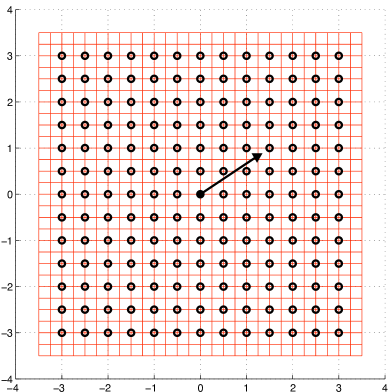
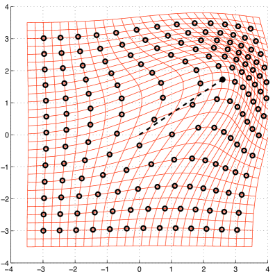
Figure 3: Dragging effect of one momentum-carrying landmark $q^{1}$ (bullet $\bullet$) on a grid of landmarks (circles $\circ$), with $\gamma(x)=\exp(-\frac{1}{2}\frac{x^{2}}{\sigma^{2}})$, $\sigma=1.5$. Left: initial configuration, with initial momentum $p_{1}=(2.7,1.8)$ also shown. Right: configuration after one unit of time, with trajectory of $q^{1}$ also shown; the grid represents the diffeomorphism $\varphi_{01}^{v}$, obtained by integrating $\alpha^{\mathrm{hor}}$ in time.

Negative curvature can be seen by the divergence of geodesics. If you imagine slightly changing the direction of $p_{1}$ in Figure 3, the final configuration of the landmark points (say, after one unit of time) will differ greatly from the one caused by the original value of $p_{1}$. Also, if you imagine $q^{1}$ moving along two nearby parallel straight lines, the differential effect on the cloud of other points accumulates so that the final configurations will differ everywhere; thus, even though the initial landmark configurations are close, the final configurations will be far away. In general, the last negative term in the curvature expresses the same effect: the global drag effect of each point results in a kind of turbulent mixing of all the other points (think of a kitchen mixer the motion of whose blades mixes the whole bowl).

Proposition 14 simplifies in the case of $\mathcal{L}=\mathcal{L}^{2}(\mathbb{R}^{D})$ (two landmarks only). We shall write:

$$\alpha_{1}^{\parallel} :=\langle\alpha_{1},u^{12}\rangle, \alpha_{1}^{\perp} :=\alpha_{1}-\alpha_{1}^{\parallel}\,u^{12}, \beta_{1}^{\parallel} :=\langle\beta_{1},u^{12}\rangle, \beta_{1}^{\perp} :=\beta_{1}-\beta_{1}^{\parallel}\,u^{12}.$$ (56)

Proposition 15.

In the case of $\mathcal{L}=\mathcal{L}^{2}(\mathbb{R}^{D})$, when $\alpha,\beta\in(T^{\ast}_{q}\mathcal{L})_{1}$ the numerator and denominator of sectional curvature are given by, respectively:

$$R(\alpha^{\sharp},\beta^{\sharp},\beta^{\sharp},\alpha^{\sharp})=R_{4} =-\frac{3}{4}\,\gamma_{0}\,\frac{\gamma_{0}-\gamma_{12}}{\gamma_{0}+\gamma_{12}}\,\big{(}\gamma^{\prime}_{12}\big{)}^{2}\,\big{\|}\beta_{1}^{\parallel}\alpha_{1}^{\perp}-\alpha_{1}^{\parallel}\beta_{1}^{\perp}\big{\|}^{2},$$ (57)

$$\|\alpha\|^{2}_{T^{\ast}\mathcal{L}}\,\|\beta\|_{T^{\ast}\mathcal{L}}^{2}-\langle\alpha,\beta\rangle_{T^{\ast}\mathcal{L}}^{2} =\gamma_{0}^{2}\Big{(}\big{\|}\beta_{1}^{\parallel}\alpha_{1}^{\perp}-\alpha_{1}^{\parallel}\beta_{1}^{\perp}\big{\|}^{2}+{\textstyle\frac{1}{2}}\big{\|}\beta_{1}^{\perp}\otimes\alpha_{1}^{\perp}-\alpha_{1}^{\perp}\otimes\beta_{1}^{\perp}\big{\|}^{2}\Big{)}.$$ (58)

Again we have used the inner product of tensor products $\langle v_{1}\otimes w_{1},v_{2}\otimes w_{2}\rangle:=\langle v_{1},v_{2}\rangle\langle w_{1},w_{2}\rangle$.

Proof.

It is the case that $R_{4}=-\frac{3}{4}\|H^{2}\|^{2}(\mathbf{K}^{-1})_{22}$ (matrices $H^{a}$ were defined in Proposition 14). But $(\mathbf{K}^{-1})_{22}=(\gamma_{0}^{2}-\gamma_{12}^{2})^{-1}\gamma_{0}$, whereas from Proposition 14 we have

$$\|H^{2}\|^{2}=(\gamma_{0}-\gamma_{12})^{2}\big{(}\langle\alpha_{1},\nabla K^{12}\rangle^{2}\|\beta_{1}\|^{2}+\langle\beta_{1},\nabla K^{12}\rangle^{2}\|\alpha_{1}\|^{2}-2\langle\alpha_{1},\nabla K^{12}\rangle\langle\beta_{1},\nabla K^{12}\rangle\langle\alpha_{1},\beta_{1}\rangle\big{)},$$

where $\nabla K^{12}=\gamma^{\prime}_{12}u^{12}$ by (52). Inserting expressions (56) into the above formula yields (57). From Proposition 11 we have that the denominator is given by $\gamma_{0}^{2}(\|\alpha_{1}\|^{2}\|\beta_{1}\|^{2}-\langle\alpha_{1},\beta_{1}\rangle^{2})$; again, inserting (56) into such formula yields (58). ∎

We will generalize the above results in the next section.

5 Landmark geometry with two nonzero momenta

The complexity of the formula for curvature reflects a real complexity in the geometry of the landmark space. But there is one case in which the geometry such space can be analyzed quite completely. This is when there are only two nonzero momenta along a geodesic. To put this in context, we first introduce a basic structural relation between landmark spaces.

5.1 Submersions between landmark spaces

Instead of labeling the landmarks as $1,2,\cdots,N$, one can use any finite index set $\mathcal{A}$ and label the landmarks as $q^{a}$ with $a\in\mathcal{A}$. And instead of calling the landmark space $\mathcal{L}^{N}$, we can call it $\mathcal{L}^{\mathcal{A}}$. Now suppose we have a subset $\mathcal{B}\subset\mathcal{A}$. Then there is a natural projection $\pi:\mathcal{L}^{\mathcal{A}}\rightarrow\mathcal{L}^{\mathcal{B}}$ gotten by forgetting about the points with labels in $\mathcal{A}-\mathcal{B}$. In the metrics we have been discussing this is a submersion. In fact, the kernel of $d\pi$, the vertical subspace of $T\mathcal{L}^{\mathcal{A}}$, is the space of vectors $v^{a}$ such that $v^{a}=0$ if $a\in\mathcal{B}$. Its perpendicular in $T^{\ast}$ is:

$$(T^{\ast}\mathcal{L}^{\mathcal{A}})_{\mathcal{B}}:=\big{\{}p\in T^{\ast}\mathcal{L}^{\mathcal{A}}\,\big{|}p_{a}=0\mbox{ for }a\in\mathcal{A}-\mathcal{B}\big{\}}$$

so the orthogonal complement of ker($d\pi$) in $T\mathcal{L}^{\mathcal{A}}$ is the space of vectors $p^{\sharp}$ where $p$ is in $(T^{\ast}\mathcal{L}^{\mathcal{A}})_{\mathcal{B}}$. On this subspace, the norm is just

$$\sum_{b,b^{\prime}\in\mathcal{B}}K(q^{b}-q^{b^{\prime}})\langle p_{b},p_{b^{\prime}}\rangle$$

whether $p^{\sharp}$ is taken to be a tangent vector to $\mathcal{A}$ or to $\mathcal{B}$. In other words, the horizontal subspace for the submersion $\pi$ is the subbundle $(T^{\ast}\mathcal{L}^{\mathcal{A}})_{\mathcal{B}}^{\sharp}\subset T\mathcal{L}^{\mathcal{A}}$ of tangent vectors $p^{\sharp}$ where $p$ has zero components in $\mathcal{A}-\mathcal{B}$ and this has the same metric as the tangent space to $\mathcal{L}^{\mathcal{B}}$. In particular, from the general theory of submersions, we know that every geodesic in $\mathcal{L}^{\mathcal{B}}$ beginning at some point $\pi(\{q^{a}\})$ has a unique lift to a horizontal geodesic in $\mathcal{L}^{\mathcal{A}}$ starting at $\{q^{a}\}$. The picture to have is that all the landmark spaces form a sort of inverse system of spaces whose inverse limit is the group of diffeomorpisms of $\mathbb{R}^{D}$.

We don’t want to pursue this is in general, but rather we will study the special case where the cardinality of $\mathcal{B}$ is two. We might as well, then, go back to our former terminology and consider the map $\pi:\mathcal{L}^{N}\rightarrow\mathcal{L}^{2}$ gotten by mapping an $N$-tuple $(q^{1},q^{2},\cdots,q^{N})$ to the pair $(q^{1},q^{2})$. Moreover, we want to consider only the case in which the kernel $K$ is rotationally invariant as in (K4). A basic quantity in all that follows is the distance $\rho:=\|q^{1}-q^{2}\|$ between the two momentum bearing points.

5.2 Two momentum geodesics

Remarkably, we can describe, more or less explicitly, all the geodesics which arise as horizontal lifts from this map. These are the geodesics with nonzero momenta only at $q^{1}$ and $q^{2}$. Moreover, the formula for sectional curvature for the 2-plane spanned by any two horizontal vectors can be analyzed. This analysis was started in the PhD thesis of the first author [23] and has been pursued further in [22].

The metric tensor of $\mathcal{L}=\mathcal{L}^{2}(\mathbb{R}^{D})$ in coordinates is obtained by inverting the $2\times 2$ matrix K:

$$\mathbf{K}=\left[\begin{array}[]{cc}\gamma_{0}&\gamma(\rho)\\ \gamma(\rho)&\gamma_{0}\end{array}\right]\;\;\Longrightarrow\;\;\left\{\begin{array}[]{l}(\mathbf{K}^{-1})_{11}=(\mathbf{K}^{-1})_{22}=(\gamma_{0}^{2}-\gamma(\rho)^{2})^{-1}\gamma_{0}\\ (\mathbf{K}^{-1})_{12}=(\mathbf{K}^{-1})_{21}=-(\gamma_{0}^{2}-\gamma(\rho)^{2})^{-1}\gamma(\rho)\end{array}\right.,$$ (59)

so that the cometric and metric, for all covectors $\alpha,\beta\in T^{\ast}_{q}\mathcal{L}$ and vectors $v,w\in T_{q}\mathcal{L}$, are simply:

$$g^{-1}(\alpha,\beta) =\gamma_{0}\big{(}\langle\alpha_{1},\beta_{1}\rangle+\langle\alpha_{2},\beta_{2}\rangle\big{)}+\gamma(\rho)\big{(}\langle\alpha_{1},\beta_{2}\rangle+\langle\alpha_{2},\beta_{1}\rangle\big{)},$$ (60)

$$g(v,w) =\frac{1}{\gamma_{0}^{2}-\gamma(\rho)^{2}}\Big{[}\,\gamma_{0}\big{(}\langle v^{1},w^{1}\rangle+\langle v^{2},w^{2}\rangle\big{)}-\gamma(\rho)\big{(}\langle v^{1},w^{2}\rangle+\langle v^{2},w^{1}\rangle\big{)}\Big{]}.$$

The geometry of the two-point space is best understood by changing variables for the landmark coordinates $(q^{1},q^{2})$ and the momentum $(p_{1},p_{2})$ to their means and semi-differences, that is:

$$\overline{q}:= \;\frac{q^{1}+q^{2}}{2}, \delta q:= \;\frac{q^{1}-q^{2}}{2}, \overline{p}:= \;\frac{p_{1}+p_{2}}{2}, \delta p:= \;\frac{p_{1}-p_{2}}{2},$$

$$\mbox{so that: }\qquad q^{1}= \;\overline{q}+\delta q, q^{2}= \;\overline{q}-\delta q, p_{1}= \;\overline{p}+\delta p, p_{2}= \;\overline{p}-\delta p.$$

Then the cometric (60) becomes:

$$g^{-1}\big{(}(\overline{\alpha},\delta\alpha),(\overline{\beta},\delta\beta)\big{)} =2\big{(}\gamma_{0}+\gamma(\rho)\big{)}\,\big{\langle}\overline{\alpha},\overline{\beta}\big{\rangle}+2\big{(}\gamma_{0}-\gamma(\rho)\big{)}\,\big{\langle}\delta{\alpha},\delta{\beta}\big{\rangle}.$$ (61)

With these coordinates, the two-point landmark space becomes a product $\overline{V}\times V_{\delta}$ in which all fibers $\overline{V}\times\{\delta q_{0}\}$ are flat Euclidean spaces though with variable scales, all fibers $\{\overline{q}_{0}\}\times V_{\delta}$ are conformally flat metrics sitting on the manifold $\mathbb{R}^{D}-\{0\}$ and the tangent spaces of the two factors are orthogonal.

Proposition 16.

In terms of means and semi-differences, the geodesic equations for $\mathcal{L}^{2}(\mathbb{R}^{D})$ are:

$$\dot{\overline{q}} =\big{(}\gamma_{0}+\gamma(\rho)\big{)}\,\overline{p}, \dot{\overline{p}} =0,$$ (62)

$$\dot{\delta q} =\big{(}\gamma_{0}-\gamma(\rho)\big{)}\,\delta p, \dot{\delta p} =-2\frac{\gamma^{\prime}(\rho)}{\rho}\big{(}\|\overline{p}\|^{2}-\|\delta p\|^{2}\big{)}\,\delta q.$$

The above result is proven by direct computation. We can solve these equations in four steps.

1. First the linear momentum $\overline{p}$ is a constant, so “center of mass” $\overline{q}$ moves in a straight line parallel to this constant:

$$\overline{q}(t)=\overline{q}(0)+\Big{(}\int_{0}^{t}\big{(}\gamma_{0}+\gamma(\rho(\tau))\big{)}d\tau\Big{)}\,\overline{p}.$$ (63)

2. Secondly, if we treat vectors $\delta q$ and $\delta p$ as 1-forms in $\mathbb{R}^{D}$, equations (62) also show that:

$$(\delta q\wedge\delta p)^{\centerdot}=\dot{\delta q}\wedge\delta p+\delta q\wedge\dot{\delta p}=[\text{(scalar)}\,\delta p]\wedge\delta p+\delta q\wedge[\text{(scalar)}\,\delta q]=0,$$

so the angular momentum 2-form $\delta q\wedge\delta p\in\bigwedge^{2}\mathbb{R}^{D}$ is constant; we write this as $\omega\,e^{1}\wedge e^{2}$ where $\omega$ is the nonnegative real magnitude of the angular momentum and $(e^{1},e^{2})$ is an orthonormal pair. Then it follows that:

$$\delta q(t)=\tfrac{1}{2}\rho(t)\big{[}\cos\big{(}\theta(t)\big{)}e^{1}+\sin\big{(}\theta(t)\big{)}e^{2}\big{]},\quad\text{for some function }\theta(t).$$

3. Thirdly, we can express $\theta(t)$ as an integral:

$$\dot{\delta q} =\tfrac{1}{2}\dot{\rho}\big{[}\cos(\theta)e^{1}+\sin(\theta)e^{2}\big{]}+\tfrac{1}{2}\rho\dot{\theta}\big{[}-\sin(\theta)e^{1}+\cos(\theta)e^{2}\big{]},\quad\text{so}$$

$$\dot{\delta q}\wedge\delta q =-\tfrac{1}{4}\rho^{2}\dot{\theta}\,e^{1}\wedge e^{2},\quad\text{as well as (from~{}\eqref{2ptgeodeq}):}$$

$$\dot{\delta q}\wedge\delta q =\big{(}\gamma_{0}-\gamma(\rho)\big{)}\delta p\wedge\delta q=-\omega\,\big{(}\gamma_{0}-\gamma(\rho)\big{)}\,e^{1}\wedge e^{2};$$

combining the second and third lines, we find:

$$\theta(t)=\theta(0)+4\omega\int_{0}^{t}\frac{\gamma_{0}-\gamma(\rho(\tau))}{\rho(\tau)^{2}}\,d\tau;$$ (64)

note that by (K1) and (K2) it is the case that $\gamma_{0}\geq\gamma(\rho)$ for any $\rho\geq 0$, so $\theta$ is a monotone increasing function if $\omega\not=0$, otherwise it is a constant.

4. The last step is to solve for $\rho(t)$. This can be done using conservation of energy [16, p. 51]. Equations (62) are in fact the cogeodesic equations for the Hamiltonian $\mathcal{H}(p,q)$ of section 4.1, which we may rewrite in terms of means and semi-differences as

$$\mathcal{H}=\big{(}\gamma_{0}+\gamma(\rho)\big{)}\|\overline{p}\|^{2}+\big{(}\gamma_{0}-\gamma(\rho)\big{)}\|\delta p\|^{2}$$

by (61); hence this function of $\rho$ and $\|\delta p\|$ is a constant ($\overline{p}$ is also a constant). Then we calculate:

$$(\rho^{2})^{\centerdot} =4\langle\delta q,\delta q\rangle^{\centerdot}=8\langle\dot{\delta q},\delta q\rangle=8\big{(}\gamma_{0}-\gamma(\rho)\big{)}\langle\delta p,\delta q\rangle\quad\Longrightarrow\quad\dot{\rho}=4\frac{\gamma_{0}-\gamma(\rho)}{\rho}\langle\delta p,\delta q\rangle.$$

But:

$$\quad\langle\delta p,\delta q\rangle^{2}+\omega^{2} =\langle\delta p,\delta q\rangle^{2}+\|\delta p\wedge\delta q\|^{2}=\|\delta p\|^{2}\cdot\|\delta q\|^{2}=\frac{\rho^{2}}{4}\bigg{(}\frac{\mathcal{H}-(\gamma_{0}+\gamma(\rho))\|\overline{p}\|^{2}}{\gamma_{0}-\gamma(\rho)}\bigg{)},$$

$$\Longrightarrow\quad\dot{\rho} =2\frac{\sqrt{\gamma_{0}-\gamma(\rho)}}{\rho}\sqrt{\rho^{2}\big{[}\mathcal{H}-\big{(}\gamma_{0}+\gamma(\rho)\big{)}\|\overline{p}\|^{2}\big{]}-4\omega^{2}\big{(}\gamma_{0}-\gamma(\rho)\big{)}}.$$

This means that the function $\rho(t)$ is the solution of:

$$t =\int_{\rho(0)}^{\rho(t)}\frac{x\,dx}{2\sqrt{F(x)}},\quad\mbox{where:}\quad F(x):=\mathcal{H}\,x^{2}\big{(}\gamma_{0}-\gamma(x)\big{)}-\|\overline{p}\|^{2}x^{2}\big{(}\gamma_{0}^{2}-\gamma(x)^{2}\big{)}-4\omega^{2}\big{(}\gamma_{0}-\gamma(x)\big{)}^{2}.$$ (65)

Summary.

If we fix constants $\mathcal{H}$, $\overline{p}$, $\omega$, $\rho(0)$, $\theta(0)$, $q^{a}(0)$ (for all $a$), we can first integrate (65) to get $\rho(t)$ (the separation of $q^{1}$ and $q^{2}$), then integrate (64) to find their relative angle $\theta(t)$, then integrate (63) to get their center of mass $\overline{q}(t)$. This gives the trajectories of $q^{1}$ and $q^{2}$. The remaining points are dragged along as solutions of: $\tfrac{d}{dt}q^{a}(t)=\gamma\big{(}\|q^{a}(t)-q^{1}(t)\|\big{)}p_{1}(t)+\gamma\big{(}\|q^{a}(t)-q^{2}(t)\|\big{)}p_{2}(t).$

As worked out in [22], one can classify the global behavior of these geodesics into two types. One is the scattering type in which $q^{1},q^{2}$ diverge from each other as time goes to either $\pm\infty$. This occurs if the linear or angular momentum is large enough compared to the energy. In the other case where the energy is large enough compared to both momenta, they come together asymptotically at either $t=+\infty$ or $-\infty$, diverging at the other limit. In both cases, they may spiral around each other an arbitrarily large number of times (see Figure 4).

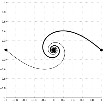
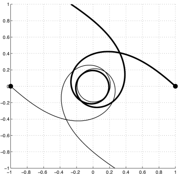
Figure 4: Converging and diverging trajectories for two landmarks in two dimensions. In these examples $\gamma(x)=\exp(-\frac{1}{2}x^{2})$, $(q^{1}(0),q^{2}(0))=((1,0),(-1,0))$, $(p_{1}(0),p_{2}(0))=((-10,8.6),(10,-8.6))$ for the graph on the left, $(p_{1}(0),p_{2}(0))=((-10,9),(10,-9))$ for the graph on the right. The thick and thin lines are, respectively, the trajectories of the first and second landmarks.

5.3 Decomposing curvature

Next we consider $\mathcal{L}^{N}(\mathbb{R}^{D})$: we want to compute the sectional curvature $R(\alpha^{\sharp},\beta^{\sharp},\beta^{\sharp},\alpha^{\sharp})$ for cotangent vectors that are nonzero at only $(q^{1},q^{2})$. Also, we will use the notation $u:=\frac{q^{1}-q^{2}}{\|q^{1}-q^{2}\|}$ for the unit vector from $q^{2}$ to $q^{1}$ as well as $\rho=\|q^{1}-q^{2}\|$ for their distance. Similarly to (54), we will also want to decompose any vector in $\eta\in\mathbb{R}^{D}$ into its parts tangent to $u$ and perpendicular to $u$:

$$\eta^{\parallel}:=\langle\eta,u\rangle,\quad\mathrm{and}\quad\eta^{\bot}:=\eta-\eta^{\parallel}\,u.$$

Once again note that $\eta^{\parallel}$ is a scalar whereas $\eta^{\perp}$ is a vector. Following the notation used to describe geodesics above, for any $\alpha\in(T^{\ast}_{q}\mathcal{L})_{1,2}:=\big{\{}\eta\in T^{\ast}_{q}\mathcal{L}\,\big{|}\,\eta_{a}=0\mbox{ for }a>2\big{\}}$, we write $\overline{\alpha}=\tfrac{1}{2}(\alpha_{1}+\alpha_{2})$ and $\delta\alpha=\tfrac{1}{2}(\alpha_{1}-\alpha_{2})$.

Proposition 17.

In $\mathcal{L}^{N}(\mathbb{R}^{D})$ for any pair $\alpha,\beta\in(T^{\ast}_{q}\mathcal{L})_{1,2}$, the terms $R_{1},R_{2}$ and $R_{3}$ in the numerator of sectional curvature can be written as

$$R_{1} =4\big{(}\gamma_{0}-\gamma(\rho)\big{)}^{2}\gamma^{\prime\prime}(\rho)\,\big{\langle}\delta\alpha^{\parallel}\beta_{1}-\delta\beta^{\parallel}\alpha_{1},\delta\alpha^{\parallel}\beta_{2}-\delta\beta^{\parallel}\alpha_{2}\big{\rangle}$$

$$\;\;\;\;+4\big{(}\gamma_{0}-\gamma(\rho)\big{)}^{2}\,\frac{\gamma^{\prime}(\rho)}{\rho}\,\big{\langle}\delta\alpha^{\bot}\otimes\beta_{1}-\delta\beta^{\bot}\otimes\alpha_{1},\delta\alpha^{\bot}\otimes\beta_{2}-\delta\beta^{\bot}\otimes\alpha_{2}\big{\rangle},$$

$$R_{2} =-4\big{(}\gamma_{0}-\gamma(\rho)\big{)}\,\gamma^{\prime}(\rho)^{2}\,\big{\langle}\delta\alpha^{\parallel}\beta_{1}-\delta\beta^{\parallel}\alpha_{1},\delta\alpha^{\parallel}\beta_{2}-\delta\beta^{\parallel}\alpha_{2}\big{\rangle},$$

$$R_{3} =\frac{\gamma_{0}-\gamma(\rho)}{2}\,\gamma^{\prime}(\rho)^{2}\big{[}\big{(}\langle\alpha_{1},\beta_{2}\rangle+\langle\beta_{1},\alpha_{2}\rangle\big{)}^{2}-4\langle\alpha_{1},\alpha_{2}\rangle\langle\beta_{1},\beta_{2}\rangle\big{]}.$$

We need the following result.

Lemma 18.

For any $\alpha\in(T^{\ast}_{q}\mathcal{L})_{1,2}$, the discrete strain $S^{12}(\alpha)$ is given by:

$$S^{12}(\alpha)=2\big{(}\gamma_{0}-\gamma(\rho)\big{)}\delta\alpha.$$ (66)

For any pair $\alpha,\beta\in(T^{\ast}_{q}\mathcal{L})_{1,2}$ it is the case that $F_{a}(\alpha,\beta)=0$ for $a>2$, whereas

$$F_{1}(\alpha,\beta) =-F_{2}(\alpha,\beta)=\frac{\gamma^{\prime}(\rho)}{2}\big{(}\langle\alpha_{1},\beta_{2}\rangle+\langle\beta_{1},\alpha_{2}\rangle\big{)}u.$$ (67)

Also,

$$D^{1}(\alpha,\beta)=2\big{(}\gamma_{0}-\gamma(\rho)\big{)}\,\gamma^{\prime}(\rho)\,\delta\alpha^{\parallel}\,\beta_{2},\qquad D^{2}(\alpha,\beta)=2\big{(}\gamma_{0}-\gamma(\rho)\big{)}\,\gamma^{\prime}(\rho)\,\delta\alpha^{\parallel}\,\beta_{1}.$$ (68)

Remark.

We are not interested in $D^{a}(\alpha,\beta)$ for $a>2$ since the terms in formula (43) where they appear are zero (because $F_{a}(\alpha,\beta)=0$ for $a>2$).

Proof of Lemma 18..

The formula for the discrete strain results from:

$$S^{12}(\alpha)=(\alpha^{\sharp})^{1}-(\alpha^{\sharp})^{2}=\textstyle\sum_{b}(K^{1b}-K^{2b})\alpha_{b}=\gamma_{0}\alpha_{1}+\gamma(\rho)\alpha_{2}-\gamma(\rho)\alpha_{1}-\gamma_{0}\alpha_{2}=2\big{(}\gamma_{0}-\gamma(\rho)\big{)}\delta\alpha.$$

The values for $F$ follow immediately from formula (39) and $\nabla K^{12}=\gamma^{\prime}(\rho)\,u$. Note that:

$$C^{12}(\alpha)=C^{21}(\alpha)=\big{\langle}S^{12}(\alpha),\nabla K^{12}\big{\rangle}=\big{\langle}2\big{(}\gamma_{0}-\gamma(\rho)\big{)}\delta\alpha,\gamma^{\prime}(\rho)u\big{\rangle}=2\big{(}\gamma_{0}-\gamma(\rho)\big{)}\gamma^{\prime}(\rho)\,\delta\alpha^{\parallel},\mbox{ so}$$

$D^{1}(\alpha,\beta)\!=\!C^{12}(\alpha)\beta_{2}\!=\!2(\gamma_{0}\!-\!\gamma(\rho))\gamma^{\prime}(\rho)\delta\alpha^{\parallel}\beta_{2}$ and $D^{2}(\alpha,\beta)\!=\!C^{21}(\alpha)\beta_{1}\!=\!2(\gamma_{0}\!-\!\gamma(\rho))\gamma^{\prime}(\rho)\delta\alpha^{\parallel}\beta_{1}$. ∎

Proof of Proposition 17.

The $R_{1}$ expression follows by substituting the expressions in (66) into formula (55), noting that the only non-zero terms in the latter are for $(a,b)=(1,2)$ and $(a,b)=(2,1)$.

By Theorem 9 and the fact that $F_{2}=-F_{1}$ from Lemma 18, $R_{2}$ is given by

$$R_{2}= \,\big{\langle}D^{1}(\alpha,\alpha)-D^{2}(\alpha,\alpha),F_{1}(\beta,\beta)\big{\rangle}+\big{\langle}D^{1}(\beta,\beta)-D^{2}(\beta,\beta),F_{1}(\alpha,\alpha)\big{\rangle}$$

$$-\big{\langle}D^{1}(\alpha,\beta)-D^{2}(\alpha,\beta)+D^{1}(\beta,\alpha)-D^{2}(\beta,\alpha),F_{1}(\alpha,\beta)\big{\rangle}.$$ (69)

Again by Lemma 18 we have that $D^{1}(\eta,\zeta)-D^{2}(\eta,\zeta)=-4\big{(}\gamma_{0}-\gamma(\rho)\big{)}\gamma^{\prime}(\rho)\,\delta\eta^{\parallel}\,\delta\zeta$ for any pair $\eta,\zeta\in(T^{\ast}_{q}\mathcal{L})_{1,2}$, while $F_{1}(\eta,\zeta)=\frac{1}{2}\gamma^{\prime}(\rho)\big{(}\langle\eta_{1},\zeta_{2}\big{\rangle}+\langle\eta_{2},\zeta_{1}\rangle\big{)}u.$ Applying this to all the terms we get the expression for $R_{2}$ in the statement of the proposition.

As far as $R_{3}$ is concerned, by Theorem 9:

$$R_{3} =\gamma_{0}\big{[}\langle F_{1}(\alpha,\beta),\!F_{1}(\alpha,\beta)\rangle\!-\!\langle F_{1}(\alpha,\alpha),\!F_{1}(\beta,\beta)\rangle\big{]}\!+\!\gamma(\rho)\big{[}\langle F_{1}(\alpha,\beta),\!F_{2}(\alpha,\beta)\rangle-\!\langle F_{1}(\alpha,\alpha)\!,\!F_{2}(\beta,\beta)\rangle\big{]}$$

$$\;\;\;+\gamma(\rho)\big{[}\langle F_{2}(\alpha,\beta),\!F_{1}(\alpha,\beta)\rangle\!-\!\langle F_{2}(\alpha,\alpha),\!F_{1}(\beta,\beta)\rangle\big{]}\!+\!\gamma_{0}\big{[}\langle F_{2}(\alpha,\beta),\!F_{2}(\alpha,\beta)\rangle-\!\langle F_{2}(\alpha,\alpha)\!,\!F_{2}(\beta,\beta)\rangle\big{]}$$

$$=2(\gamma_{0}-\gamma(\rho))\big{[}\langle F_{1}(\alpha,\beta),F_{1}(\alpha,\beta)\rangle-\langle F_{1}(\alpha,\alpha),F_{1}(\beta,\beta)\rangle\big{]}$$

$$=\textstyle\frac{\gamma_{0}-\gamma(\rho)}{2}(\gamma^{\prime}(\rho))^{2}\big{[}(\langle\alpha_{1},\beta_{2}\rangle+\langle\beta_{1},\alpha_{2}\rangle)^{2}-4\langle\alpha_{1},\alpha_{2}\rangle\langle\beta_{1},\beta_{2}\rangle\big{]},$$

where we have used the fact that $F_{2}=-F_{1}$, by equation (67). This completes the proof. ∎

The expressions provided by Proposition 17 become much clearer if we go over to means and semi-differences, i.e. if we use the substitutions:

$$\alpha_{1}=\overline{\alpha}+\delta\alpha,\quad\alpha_{2}=\overline{\alpha}-\delta\alpha,\quad\beta_{1}=\overline{\beta}+\delta\beta,\quad\beta_{2}=\overline{\beta}-\delta\beta.$$ (70)

Corollary 19.

For any $\alpha,\beta\in(T^{\ast}_{q}\mathcal{L})_{1,2}$, with $\mathcal{L}=\mathcal{L}^{N}(\mathbb{R}^{D})$, it is the case that:

$$R_{1} =4\big{(}\gamma_{0}-\gamma(\rho)\big{)}^{2}\gamma^{\prime\prime}(\rho)\,\big{(}\|\delta\beta^{\parallel}\overline{\alpha}-\delta\alpha^{\parallel}\overline{\beta}\|^{2}-\|\delta\beta^{\parallel}\delta\alpha-\delta\alpha^{\parallel}\delta\beta\|^{2}\big{)}$$

$$\;\;\;\;+4\big{(}\gamma_{0}-\gamma(\rho)\big{)}^{2}\frac{\gamma^{\prime}(\rho)}{\rho}\big{(}\|\delta\beta^{\bot}\otimes\overline{\alpha}-\delta\alpha^{\bot}\otimes\overline{\beta}\|^{2}-\|\delta\beta^{\bot}\otimes\delta\alpha-\delta\alpha^{\bot}\otimes\delta\beta\|^{2}\big{)},$$

$$R_{2} =-4\big{(}\gamma_{0}-\gamma(\rho)\big{)}\gamma^{\prime}(\rho)^{2}\,\big{(}\|\delta\beta^{\parallel}\overline{\alpha}-\delta\alpha^{\parallel}\overline{\beta}\|^{2}-\|\delta\beta^{\parallel}\delta\alpha-\delta\alpha^{\parallel}\delta\beta\|^{2}\big{)},$$

$$R_{3} =\big{(}\gamma_{0}-\gamma(\rho)\big{)}\gamma^{\prime}(\rho)^{2}\,\big{(}2\|\delta\beta\otimes\overline{\alpha}-\delta\alpha\otimes\overline{\beta}\|^{2}-\|\overline{\beta}\otimes\overline{\alpha}-\overline{\alpha}\otimes\overline{\beta}\|^{2}-\|\delta\beta\otimes\delta\alpha-\delta\alpha\otimes\delta\beta\|^{2}\big{)}.$$

Proof.

By insertion of formulae (70) it is easily seen that

$$\big{\langle}\delta\alpha^{\parallel}\beta_{1}-\delta\beta^{\parallel}\alpha_{1},\delta\alpha^{\parallel}\beta_{2}-\delta\beta^{\parallel}\alpha_{2}\big{\rangle} =\|\delta\beta^{\parallel}\overline{\alpha}-\delta\alpha^{\parallel}\overline{\beta}\|^{2}-\|\delta\beta^{\parallel}\delta\alpha-\delta\alpha^{\parallel}\delta\beta\|^{2},$$

$$\big{\langle}\delta\alpha^{\bot}\otimes\beta_{1}-\delta\beta^{\bot}\otimes\alpha_{1},\delta\alpha^{\bot}\otimes\beta_{2}-\delta\beta^{\bot}\otimes\alpha_{2}\big{\rangle} =\|\delta\beta^{\bot}\otimes\overline{\alpha}-\delta\alpha^{\bot}\otimes\overline{\beta}\|^{2}\!-\|\delta\beta^{\bot}\otimes\delta\alpha-\delta\alpha^{\bot}\otimes\delta\beta\|^{2}\!\!,$$

so the new expressions for $R_{1}$ and $R_{2}$ follow immediately. Also:

$$\big{[}\langle\alpha_{1}, \beta_{2}\rangle+\langle\beta_{1},\alpha_{2}\rangle\big{]}^{2}-4\langle\alpha_{1},\alpha_{2}\rangle\langle\beta_{1},\beta_{2}\rangle$$

$$=\big{[}2(\langle\overline{\alpha},\overline{\beta}\rangle-\langle\delta\alpha,\delta\beta\rangle)\big{]}^{2}-4\big{(}\langle\overline{\alpha},\overline{\alpha}\rangle-\langle\delta\alpha,\delta\alpha\rangle\big{)}\big{(}\langle\overline{\beta},\overline{\beta}\rangle-\langle\delta\beta,\delta\beta\rangle\big{)}$$

$$=-2\big{[}2(\langle\overline{\alpha},\overline{\alpha}\rangle\langle\overline{\beta},\overline{\beta}\rangle-\langle\overline{\alpha},\overline{\beta}\rangle^{2})\big{]}-2\big{[}2(\langle\delta\alpha,\delta\alpha\rangle\langle\delta\beta,\delta\beta\rangle-\langle\delta\alpha,\delta\beta\rangle^{2})\big{]}$$

$$\quad+4\big{[}\langle\overline{\alpha},\overline{\alpha}\rangle\langle\delta\beta,\delta\beta\rangle+\langle\overline{\beta},\overline{\beta}\rangle\langle\delta\alpha,\delta\alpha\rangle-2\langle\overline{\alpha},\overline{\beta}\rangle\langle\delta\alpha,\delta\beta\rangle\big{]}$$

$$=-2\|\overline{\beta}\otimes\overline{\alpha}-\overline{\alpha}\otimes\overline{\beta}\|^{2}-2\|\delta\beta\otimes\delta\alpha-\delta\alpha\otimes\delta\beta\|^{2}+4\|\delta\beta\otimes\overline{\alpha}-\delta\alpha\otimes\overline{\beta}\|^{2}.\qed$$

The fourth term $R_{4}$ is the only one which involves the other points $q^{a},a>2$. But one has an inequality for this term involving the same expressions in $\alpha$ and $\beta$:

Proposition 20.

Any pair $\alpha,\beta\in(T^{\ast}\mathcal{L}^{N})_{1,2}$ are constant 1-forms on $\mathcal{L}^{N}$ which are pull-backs via the submersion $\mathcal{L}^{N}\rightarrow\mathcal{L}^{2}$ of constant 1-forms on $\mathcal{L}^{2}$. We can therefore consider the curvature term $R_{4}({\mathcal{L}^{N}})=-\tfrac{3}{4}\|[\alpha^{\sharp},\beta^{\sharp}]_{\mathcal{L}^{N}}\|^{2}$ on $\mathcal{L}^{N}$ and the corresponding term $R_{4}({\mathcal{L}^{2}})=-\tfrac{3}{4}\|[\alpha^{\sharp},\beta^{\sharp}]_{\mathcal{L}^{2}}\|^{2}$ on $\mathcal{L}^{2}$. Then we have the inequality:

$$R_{4}(\mathcal{L}^{N})\leq R_{4}(\mathcal{L}^{2})=-6\gamma^{\prime}(\rho)^{2}\bigg{[}\frac{\big{(}\gamma_{0}-\gamma(\rho)\big{)}^{2}}{\gamma_{0}+\gamma(\rho)}\|\delta\beta^{\parallel}\overline{\alpha}-\delta\alpha^{\parallel}\overline{\beta}\|^{2}+\big{(}\gamma_{0}-\gamma(\rho)\big{)}\,\|\delta\beta^{\parallel}\delta\alpha-\delta\alpha^{\parallel}\delta\beta\|^{2}\bigg{]}.$$

Proof.

Firstly, note that $[\alpha^{\sharp},\beta^{\sharp}]_{\mathcal{L}^{N}}$ breaks into perpendicular parts: a vertical part in the kernel of $d\pi$ and a horizontal part which is simply the horizontal lift of $[\alpha^{\sharp},\beta^{\sharp}]_{\mathcal{L}^{2}}$. This explains the inequality assertion in Proposition 20. To calculate $R_{4}(\mathcal{L}^{2})$, we use the last expression in (45), i.e.

$$R_{4}(\mathcal{L}^{2}) =\textstyle-\frac{3}{4}\sum_{a,b=1}^{2}\big{\langle}D^{a}(\alpha,\beta)-D^{a}(\beta,\alpha),D^{b}(\alpha,\beta)-D^{b}(\beta,\alpha)\big{\rangle}\,(\mathbf{K}^{-1})_{ab}$$

$$=-3\,\frac{\gamma_{0}-\gamma(\rho)}{\gamma_{0}+\gamma(\rho)}\,\gamma^{\prime}(\rho)^{2}\Big{\{}\gamma_{0}\Big{[}\|\delta\alpha^{\parallel}\beta_{1}-\delta\beta^{\parallel}\alpha_{1}\|^{2}+\|\delta\alpha^{\parallel}\beta_{2}-\delta\beta^{\parallel}\alpha_{2}\|^{2}\Big{]}$$

$$\qquad\qquad\qquad\qquad\qquad\;\;-2\gamma(\rho)\big{\langle}\delta\alpha^{\parallel}\beta_{1}-\delta\beta^{\parallel}\alpha_{1},\delta\alpha^{\parallel}\beta_{2}-\delta\beta^{\parallel}\alpha_{2}\big{\rangle}\Big{\}},$$

where we have used (59) and (68). The final result follows after inserting (70) into the above expression and performing some algebra. ∎

Note that all terms in Corollary 19 and Proposition 20 are very similar. In fact, they are all “components” of the norm $\|\alpha\wedge\beta\|^{2}$ of the 2-form whose sectional curvature is being computed. First note that we can decompose $T^{*}\mathcal{L}^{2}$ into the direct sum of three pieces, namely:

$$\delta^{\parallel}T^{*}\mathcal{L}^{2} :=\big{\{}(au,-au)\,\big{|}\,a\in\mathbb{R}\big{\}}, \dim\big{(}\delta^{\parallel}T^{*}\mathcal{L}^{2}\big{)}=1,$$

$$\delta^{\perp}T^{*}\mathcal{L}^{2} :=\big{\{}(p,-p)\,\big{|}\,p\in\mathbb{R}^{D},p\perp u\big{\}}, \dim\big{(}\delta^{\perp}T^{*}\mathcal{L}^{2}\big{)}=D-1,$$

$$\overline{T}^{*}\mathcal{L}^{2} :=\big{\{}(p,p)\,\big{|}\,p\in\mathbb{R}^{D}\big{\}}, \dim\big{(}\overline{T}^{*}\mathcal{L}^{2}\big{)}=D,$$

where as usual $u:=\frac{q^{1}-q^{2}}{\|q^{1}-q^{2}\|}$ (see Figure 5). Note that these three subspaces are orthogonal with respect to the cometric by virtue of (60). An arbitrary covector $\alpha=(\alpha_{1},\alpha_{2})\in T^{\ast}_{q}\mathcal{L}^{2}$ can be uniquely decomposed into the summation $\alpha=\alpha_{(1)}+\alpha_{(2)}+\alpha_{(3)}$, with:

$$\alpha_{(1)} :=(\delta\alpha^{\parallel}u,-\delta\alpha^{\parallel}u)\in\delta^{\parallel}T^{\ast}\mathcal{L}^{2}, \alpha_{(2)} :=(\delta\alpha^{\perp},-\delta\alpha^{\perp})\in\delta^{\perp}T^{\ast}\mathcal{L}^{2}, \alpha_{(3)} :=(\overline{\alpha},\overline{\alpha})\in\overline{T}^{\ast}\mathcal{L}^{2}.$$ (71)

So it is the case that: (i) $\alpha\in\delta^{\parallel}T^{\ast}\mathcal{L}^{2}\Leftrightarrow\delta^{\perp}\alpha=0$ and $\overline{\alpha}=0$; (ii) $\alpha\in\delta^{\perp}T^{\ast}\mathcal{L}^{2}\Leftrightarrow\delta^{\parallel}\alpha=0$ and $\overline{\alpha}=0$; (iii) $\alpha\in\overline{T}^{\ast}\mathcal{L}^{2}\Leftrightarrow\delta\alpha^{\parallel}=0$ and $\delta\alpha^{\perp}=0$.

Figure 5: Typical covectors $\alpha=(\alpha_{1},\alpha_{2})$ in spaces $\delta^{\parallel}T^{\ast}_{q}\mathcal{L}$, $\delta^{\perp}T^{\ast}_{q}\mathcal{L}$, and $\overline{T}^{\ast}_{q}\mathcal{L}$, for $\mathcal{L}=\mathcal{L}^{2}(\mathbb{R}^{2})$.

Consequently the space of 2-forms $\bigwedge^{2}T^{*}\mathcal{L}^{2}$ decomposes into the direct sum of five pieces:

$$\bigwedge^{2}T^{*}\mathcal{L}^{2} \;=\;\bigoplus_{i=1}^{5}V_{i},\mbox{ with: } V_{1} \;:=\;\delta^{\parallel}T^{*}\mathcal{L}^{2}\;\wedge\;\overline{T}^{*}\mathcal{L}^{2},$$

$$V_{2} \;:=\;\delta^{\bot}T^{*}\mathcal{L}^{2}\;\wedge\;\overline{T}^{*}\mathcal{L}^{2}, V_{3} \;:=\;\delta^{\parallel}T^{*}\mathcal{L}^{2}\;\wedge\;\delta^{\bot}T^{*}\mathcal{L}^{2},$$

$$V_{4} \;:=\;\bigwedge^{2}\big{(}\delta^{\bot}T^{*}\mathcal{L}^{2}\big{)}, V_{5} \;:=\;\bigwedge^{2}\big{(}\overline{T}^{*}\mathcal{L}^{2}\big{)}.$$

(Since $\delta^{\parallel}T^{*}\mathcal{L}^{2}$ is one-dimensional it creates no 2-forms.) Once again, note that the spaces $V_{1},\ldots,V_{5}$ are pairwise orthogonal with respect to the inner product

$$\big{\langle}\alpha\wedge\beta,\xi\wedge\eta\big{\rangle}_{\bigwedge^{2}T^{*}\mathcal{L}^{2}}:=\big{\langle}\alpha,\xi\big{\rangle}_{T^{*}\mathcal{L}^{2}}\big{\langle}\beta,\eta\big{\rangle}_{T^{*}\mathcal{L}^{2}}-\big{\langle}\alpha,\eta\big{\rangle}_{T^{*}\mathcal{L}^{2}}\big{\langle}\beta,\xi\big{\rangle}_{T^{*}\mathcal{L}^{2}},\quad\alpha,\beta,\xi,\eta\in T^{\ast}\mathcal{L}^{2}$$ (72)

by the orthogonality of $\delta^{\parallel}T^{\ast}_{q}\mathcal{L}$, $\delta^{\perp}T^{\ast}_{q}\mathcal{L}$, and $\overline{T}^{\ast}_{q}\mathcal{L}$. Any 2-form $\alpha\wedge\beta$ then decomposes into the sum of its five projections onto these subspaces and its norm squared is the sum of the norm squared of these components. Let us first give the five pieces of its norm names:

$$T_{1} :=\|\delta\beta^{\parallel}u\otimes\overline{\alpha}-\delta\alpha^{\parallel}u\otimes\overline{\beta}\|^{2},$$

$$T_{2} :=\|\delta\beta^{\bot}\otimes\overline{\alpha}-\delta\alpha^{\bot}\otimes\overline{\beta}\|^{2}, T_{3} :=\|\delta\beta^{\parallel}u\otimes\delta\alpha^{\bot}-\delta\alpha^{\parallel}u\otimes\delta\beta^{\bot}\|^{2},$$

$$T_{4} :=\|\delta\beta^{\bot}\otimes\delta\alpha^{\bot}-\delta\alpha^{\bot}\otimes\delta\beta^{\bot}\|^{2}, T_{5} :=\|\overline{\beta}\otimes\overline{\alpha}-\overline{\alpha}\otimes\overline{\beta}\|^{2}.$$

In the above definitions $\|\;\;\;\|$ indicates the Euclidean norm. We have to be careful here: we have been using Euclidean norms in $\mathbb{R}^{D}$ in all our formulas above and now we are dealing with norms in $T^{*}\mathcal{L}^{2}$; these essentially differ only by a factor, by (61). More precisely, the following result holds:

Proposition 21.

The denominator of the sectional curvature (17) for $\mathcal{L}^{2}(\mathbb{R}^{2})$ can be written as:

$$\|\alpha\wedge\beta\|_{\bigwedge^{2}T^{*}\mathcal{L}^{2}}^{2}=4\big{(}\gamma_{0}^{2}-\gamma(\rho)^{2}\big{)}(T_{1}+T_{2})+2\big{(}\gamma_{0}-\gamma(\rho)\big{)}^{2}(2T_{3}+T_{4})+2\big{(}\gamma_{0}+\gamma(\rho)\big{)}^{2}T_{5}.$$ (73)

Proof.

We may apply decomposition (71) to both $\alpha=\sum_{i=1}^{3}\alpha_{(i)}$ and $\beta=\sum_{i=1}^{3}\beta_{(i)}$, and write

$$\alpha\wedge\beta= \big{(}\alpha_{(1)}\wedge\beta_{(3)}-\beta_{(1)}\wedge\alpha_{(3)}\big{)}+\big{(}\alpha_{(2)}\wedge\beta_{(3)}-\beta_{(2)}\wedge\alpha_{(3)}\big{)}$$

$$+\big{(}\alpha_{(1)}\wedge\beta_{(2)}-\beta_{(1)}\wedge\alpha_{(2)}\big{)}+\alpha_{(2)}\wedge\beta_{(2)}+\alpha_{(3)}\wedge\beta_{(3)},$$

where the five summands on the right-hand side belong to $V_{1},\ldots,V_{5}$ respectively. We have

$$\| \alpha_{(1)}\wedge\beta_{(3)}-\beta_{(1)}\wedge\alpha_{(3)}\|^{2}_{\bigwedge^{2}T^{*}\mathcal{L}^{2}}\,\,=$$

$$=\big{\|}\alpha_{(1)}\wedge\beta_{(3)}\|^{2}_{\bigwedge^{2}T^{*}\mathcal{L}^{2}}+\big{\|}\beta_{(1)}\wedge\alpha_{(3)}\|^{2}_{\bigwedge^{2}T^{*}\mathcal{L}^{2}}-2\langle\alpha_{(1)}\wedge\beta_{(3)},\beta_{(1)}\wedge\alpha_{(3)}\rangle_{\bigwedge^{2}T^{*}\mathcal{L}^{2}}$$

$$\stackrel{{\scriptstyle(\ast)}}{{=}}4\big{(}\gamma_{0}^{2}-\gamma(\rho)^{2}\big{)}\big{[}(\delta\alpha^{\parallel})^{2}\|\overline{\beta}\|^{2}+(\delta\beta^{\parallel})^{2}\|\overline{\alpha}\|^{2}-2\,\delta\alpha^{\parallel}\delta\beta^{\parallel}\langle\alpha,\beta\rangle\big{]}=4\big{(}\gamma_{0}^{2}-\gamma(\rho)^{2}\big{)}\,T_{1},$$

where we have used (72) and (61) in step ($\ast$). The square norm of the remaining four terms is computed similarly. Orthogonality of $V_{1},\ldots,V_{5}$ finally yields (73). ∎

To express the formulas for the numerator of sectional curvature succinctly, let us also introduce abbreviations for the coefficients involving $\gamma$:

$$k_{1}(\rho) :=\big{(}\gamma_{0}-\gamma(\rho)\big{)}^{2}\gamma^{\prime\prime}(\rho), \qquad k_{2}(\rho) :=\big{(}\gamma_{0}-\gamma(\rho)\big{)}^{2}\frac{\gamma^{\prime}(\rho)}{\rho},$$ (74)

$$k_{3}(\rho) :=\big{(}\gamma_{0}-\gamma(\rho)\big{)}\gamma^{\prime}(\rho)^{2}, k_{4}(\rho) :=\frac{\big{(}\gamma_{0}-\gamma(\rho)\big{)}^{2}}{\gamma_{0}+\gamma(\rho)}\gamma^{\prime}(\rho)^{2}.$$

Note that $k_{1}$, $k_{2}$, $k_{3}$ and $k_{4}$ are all homogeneous of degree 3 in $\gamma$ and degree $-2$ in the distance $\rho$ or $d\rho$ on $\mathcal{L}^{N}$. Moreover $k_{2}$ is negative, $k_{3}$ and $k_{4}$ are positive, while $k_{1}$ may be positive or negative. For all $\gamma$ of interest, $\gamma^{\prime}$ is everywhere negative, starting at 0 decreasing to a minimum at some $\rho_{0}$, then increasing back to 0 at $\infty$. Then $k_{1}$ is negative for $\rho<\rho_{0}$ and positive for $\rho>\rho_{0}$.

The following equalities are proven by direct computation:

$$\|\delta\beta\otimes\overline{\alpha}-\delta\alpha\otimes\overline{\beta}\|^{2} =T_{1}+T_{2},$$

$$\|\delta\beta^{\perp}\otimes\delta\alpha-\delta\alpha^{\perp}\otimes\delta\beta\|^{2} =T_{3}+T_{4},$$

$$\|\delta\beta\otimes\delta\alpha-\delta\alpha\otimes\delta\beta\|^{2} =2T_{3}+T_{4}.$$

Inserting notation (74) and the above equalities into Propositions 17 and 20 immediately yields:

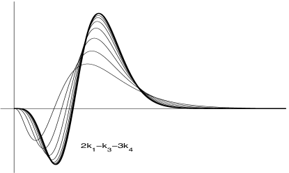
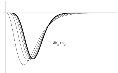
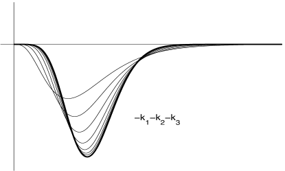
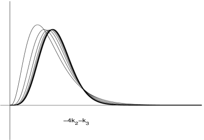
Figure 6: The coefficients of $T_{1}$ (top left), $T_{2}$ (top right), $T_{3}$ (bottom left) and $T_{4}$ (bottom right) for the Bessel kernels $\gamma$ (shown with thin lines) and the Gaussian kernel (shown with the thick line). The kernels are scaled to normalize $\gamma(0)$ and $\gamma^{\prime\prime}(0)$.

Proposition 22.

We can write the terms in the numerator of sectional curvature for $\mathcal{L}^{2}(\mathbb{R}^{D})$ as:

$$R_{1} =4k_{1}(T_{1}-T_{3})+4k_{2}(T_{2}-T_{3}-T_{4}), \qquad R_{2} =-4k_{3}(T_{1}-T_{3}),$$ (75)

$$R_{3} =k_{3}(2(T_{1}+T_{2})-2T_{3}-T_{4}-T_{5}), R_{4} =-6(k_{3}T_{3}+k_{4}T_{1}),$$

hence $R=R(\alpha^{\sharp},\beta^{\sharp},\beta^{\sharp},\alpha^{\sharp})=\sum_{i=1}^{4}R_{i}$ may be expressed as:

$$R=2\big{(}2k_{1}-k_{3}-3k_{4}\big{)}T_{1}+2\big{(}2k_{2}+k_{3}\big{)}T_{2}+4\big{(}-k_{1}-k_{2}-k_{3}\big{)}T_{3}+\big{(}-4k_{2}-k_{3}\big{)}T_{4}-k_{3}T_{5}.$$ (76)

By virtue of Proposition 20 the above proposition still holds in the case of $\mathcal{L}^{N}(\mathbb{R}^{D})$ as long as $\alpha,\beta\in(T_{q}^{\ast}\mathcal{L})_{1,2}$ and the equality signs for $R_{4}$ in (75) and $R$ in (76) are substituted by “$\leq$”. The coefficients in (76) may have all sorts of signs for peculiar kernels. However, the kernels $\gamma$ of interest are the Bessel kernels (3) and the Gaussian kernel, which is their asymptotic limit as their order goes to infinity. The coefficients for these kernels are shown in Figure 6. We see that the coefficients of $T_{2}$ and $T_{3}$ are negative while those of $T_{4}$ are positive. Henceforth, we assume we have a kernel for which this is true.

5.4 Sectional curvature of $\mathcal{L}^{2}(\mathbb{R}^{1})$

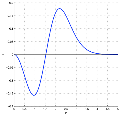
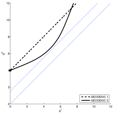
Figure 7: Left: sectional curvature $\mathcal{K}$ for  $\mathcal{L}^{2}(\mathbb{R}^{1})$ (from Proposition 23), as a function of $\rho=|q^{1}-q^{2}|$; here $\gamma(x)=\exp(-\frac{1}{2}x^{2})$. Right: two trajectories in $\mathcal{L}^{2}(\mathbb{R}^{1})$ shown in the $(q^{1},q^{2})$ plane (under the assumption that $q^{1}<q^{2}$). Both geodesics originate at $(q^{1},q^{2})=(0,4)$, and lie in the region where $\mathcal{K}>0$ (above the upper dotted line, that indicates the zero of $\mathcal{K}$ at $|q^{1}-q^{2}|\simeq 1.53$); they have different initial momenta $(p_{1},p_{2})=(1,1)$ and $(p_{1},p_{2})=(1,0.4)$, and exhibit conjugate points.

Finally, we will now explore the important example of two landmarks on the real line. In this particular case the manifold is two dimensional, so sectional curvature $\mathcal{K}$ will turn out to be independent of cotangent vectors $\alpha$ and $\beta$. In fact, given the translation invariance of the metric tensor, it will only depend on the distance $\rho=|q^{1}-q^{2}|$ between the two landmarks.

The spaces $\delta^{\parallel}T^{\ast}\mathcal{L}^{2}(\mathbb{R}^{1})$ and $\overline{T}^{\ast}\mathcal{L}^{2}(\mathbb{R}^{1})$ are one-dimensional while $\delta^{\bot}T^{\ast}\mathcal{L}^{2}(\mathbb{R}^{1})=\{0\}$. Thus

$$\bigwedge^{2}T^{\ast}\mathcal{L}^{2}(\mathbb{R}^{1})\;=\;\delta^{\parallel}T^{\ast}\mathcal{L}^{2}(\mathbb{R}^{1})\;\wedge\;\overline{T}^{\ast}\mathcal{L}^{2}(\mathbb{R}^{1})$$

and the only non-zero term in (76) is $T_{1}$. Therefore combining formulas (73) and (76) we get:

Proposition 23.

The sectional curvature of $\mathcal{L}^{2}(\mathbb{R}^{1})$ is given by

$$\mathcal{K}=\frac{2k_{1}-k_{3}-3k_{4}}{2(\gamma_{0}^{2}-\gamma(\rho)^{2})}=\frac{\gamma_{0}-\gamma(\rho)}{\gamma_{0}+\gamma(\rho)}\,\gamma^{\prime\prime}_{12}-\frac{2\gamma_{0}-\gamma(\rho)}{(\gamma_{0}+\gamma(\rho))^{2}}\big{(}\gamma^{\prime}(\rho)\big{)}^{2}.$$

The above function $\mathcal{K}$ is shown on the left-hand side of Figure 7 as a function of $\rho$, for the Gaussian kernel. The coefficient of the term $T_{1}$ in (76) is negative for $\rho$ small and positive for $\rho$ large. The “cause” of the positive curvature has been analyzed in [23]. Roughly speaking, suppose two points both want to move a fixed distance to the right. Then if they are far enough away, they can just move more or less independently (we shall refer to this as Geodesic 1). Or (i) the one in back can speed up while the one in front slows down, then (ii) when the pair are close, they move in tandem using less energy because they are close and finally (iii) the back one slows down, the front one speeds up when they near their destinations (Geodesic 2). This gives explicit conjugate points (in the sense that two points are joined by distinct geodesics) and is illustrated on the right-hand side of figure Figure 7 (where Geodesics 1 and 2 are represented, respectively, by the dashed and thick curves).

5.5 Sources of positive curvature; obstacle avoidance

There is another source of positive curvature in $\mathcal{L}^{2}$ in higher dimensions. It is clear from equation (76) and Figure 6 that any positive curvature must come from the term with $T_{1}$ or the term with $T_{4}$. As the five terms are orthogonal, we can make all of them but one zero.

For example, if we choose $\alpha=(\delta\alpha^{\parallel}u,-\delta\alpha^{\parallel}u)\in\delta^{\parallel}T^{\ast}\!\mathcal{L}$ and $\beta=(\overline{\beta},\overline{\beta})\in\overline{T}^{\ast}\!\mathcal{L}$, then it is the case that $T_{1}=(\delta\alpha^{\parallel})^{2}\|\overline{\beta}\|^{2}$ and it is the only non-zero term. Then, if $\rho$ is sufficiently large, the sectional curvature for this 2-plane is positive as discussed in the last section. Figure 8 illustrates an instance of the existence of conjugate points for two geodesics in $\mathcal{L}^{2}(\mathbb{R}^{2})$; the momenta $(p_{1},p_{2})$ of each of the two trajectories belong at all times to $\delta^{\parallel}T^{\ast}\!\mathcal{L}^{2}\oplus\overline{T}^{\ast}\!\mathcal{L}^{2}$.

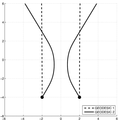
Figure 8: Existence of conjugate points in $\mathcal{L}^{2}(\mathbb{R}^{2})$, with $\gamma(x)=\exp(-\frac{1}{2}x^{2})$. Both geodesics originate at landmark set $(q^{1},q^{2})=\big{(}(-2,-4),(2,4)\big{)}$; the first one (dashed) has initial momentum $(p_{1},p_{2})=\big{(}(0,10),(0,10)\big{)}\in\overline{T}^{\ast}\mathcal{L}^{2}$ while the second one (continuous) has initial momentum $(p_{1},p_{2})=\big{(}(6,10),(-6,10)\big{)}\in\delta^{\parallel}T^{\ast}\mathcal{L}^{2}\oplus\overline{T}^{\ast}\mathcal{L}^{2}$. The geodesic trajectories exhibit conjugate points.

The other possibility is that $T_{4}$ is the non-zero term, which happens when $\alpha=(\delta\alpha^{\perp},-\delta\alpha^{\perp})\in\delta^{\perp}T^{\ast}\!\mathcal{L}$ and $\beta=(\delta\beta^{\perp},-\delta\beta^{\perp})\in\delta^{\perp}T^{\ast}\!\mathcal{L}$. We have $T_{4}=2(\|\delta\alpha^{\perp}\|^{2}\|\delta\beta^{\perp}\|^{2}-\langle\delta\alpha^{\perp},\delta\beta^{\perp}\rangle^{2})$, and for it to be nonzero it is required that $D\geq 3$ because $T_{4}$ is the norm of a 2-form in $\bigwedge^{2}\big{(}\delta^{\bot}T^{\ast}\mathcal{L}\big{)}$, which has dimension $(D-1)(D-2)/2$. The positive curvature of this section is readily seen by considering the geodesics which these vectors generate. The simplest example is the following:

Proposition 24.

The circular periodic orbit of radius $r$:

$$q^{1}(t)=(r\cos t,r\sin t),\qquad q^{2}(t)=-q^{1}(t),$$ (77)

$t\in\mathbb{R}$, is a geodesic in $\mathcal{L}^{2}(\mathbb{R}^{2})$ if and only if $r$ is the solution of the equation $\gamma_{0}-\gamma(2r)+r\gamma^{\prime}(2r)=0$.

Proof.

For orbit (77) it is the case that $\overline{q}\equiv 0$, $\delta q=q^{1}$ and $\rho\equiv 2r$; also $p_{1}=\big{(}\gamma_{0}-\gamma(\rho)\big{)}^{-1}\dot{q}^{1}$ and $p_{2}=-p_{1}$, so that $\overline{p}=0$ and $\delta p=p_{1}$. The first three equations of (62) can easily be checked; the fourth one holds if and only if $\gamma_{0}-\gamma(2r)+r\gamma^{\prime}(2r)=0$. ∎

(The above result was also proven by François-Xavier Vialard of Imperial College, London.) Orbit (77) has the property that at time $\pi$, $q^{1}$ and $q^{2}$ interchange their positions: it is a geodesic from the set of landmark points $\big{(}(r,0),(-r,0)\big{)}\in\mathcal{L}^{2}(\mathbb{R}^{2})$ to the set $\big{(}(-r,0),(r,0)\big{)}\in\mathcal{L}^{2}(\mathbb{R}^{2})$. But if these points live in $\mathbb{R}^{3}$, they can move around each other in any plane containing the points. Thus we have a circle of geodesics in $\mathcal{L}^{2}(\mathbb{R}^{3})$:

$$q^{1}(t)=(r\cos t,r\cos\theta\sin t,r\sin\theta\sin t),\qquad q^{2}(t)=-q^{1}(t)$$

all connecting $\big{(}(r,0,0),(-r,0,0)\big{)}$ to $\big{(}(-r,0,0),(r,0,0)\big{)}$, for any $\theta\in[0,2\pi)$. This is exactly like all the lines of fixed longitude connecting the north and south pole on the 2-sphere and means that one set of landmark points is a conjugate point of the other in $\mathcal{L}^{2}(\mathbb{R}^{3})$. This is the simplest example of how geodesics between landmark points must avoid collisions and so make a choice between different possible detours, leading to conjugate points and thus positive curvature.

6 Conclusions

We believe that $\mathcal{L}^{N}(\mathbb{R}^{D})$, the Riemannian manifold of $N$ landmark points in $D$ dimensions, is a fundamental object for differential geometry and that we have only scratched the surface in its study. We started with a basic formula which computes sectional curvature of a Riemannian manifold in terms of the cometric, its partial derivatives, and the metric itself (but not its derivatives). This is particularly adapted to computing curvature for manifolds which arise as submersive quotients of other manifolds and gives O’Neill’s formula as a corollary. We then applied this to derive a formula for sectional curvature of the space of landmarks. This formula is not simple but, like Arnold’s formula for curvature of Lie groups under left- (or right)-invariant metrics, splits into a sum of four terms. The four terms involve interesting intermediate expressions in the two vectors (or co-vectors) which define the section and which have relatively simple geometric interpretations. We called these the mixed force, the discrete vector strain, the scalar compression and the landmark derivative. The geodesic equation in its Hamiltonian form is quite simple and involves the force as expected. We also gave several concrete examples to illustrate the nature of these geodesics.

Finally, we have examined in detail the case of geodesics in which only one or two landmark points have non-zero momenta, and computed the curvature in sections spanned by such geodesics. We found that in this case there are essentially two sources of positive curvature. One can understand them through the non-uniqueness of geodesics joining two $N$-tuples: the first sort of non-uniqueness is caused by the two points with non-zero momentum choosing between converging in the middle of the geodesic (“car-pooling”) or moving independently and not converging; the second occurs only when $D\geq 3$ and arises when the same two points need to get around each other and must choose on which side to pass (if $D=2$, this sort non-uniqueness also occurs but comes from non-trivial topology, not curvature).

One of the most important questions left open is explore how prevalent positive curvature is in general, i.e. for geodesics in which all points carry momentum. Answering this question is central to applications of landmark space in which geodesics are actually computed. One might hope that the picture for two momenta is true in general but this is far from clear. It seems interesting to explore whether there is some sort of “index” for curvature forms — a numerical measure of how much positive vs. negative curvature is present. Another important question is to explore the shape of the coefficients in (76) for different kernels. More generally, what is the impact of different kernel types (Bessel, Gaussian, Cauchy) on the corresponding geodesics? Finally, note that all kernels have a length constant built into their definition so the geometry of the space of landmarks is far from scale invariant. Thus one should analyze what happens asymptotically when the points are very close relative to this constant or are very far from each other.

References

- [1] M. Abramowitz and I. A. Stegun. Handbook of Mathematical Functions. Dover Publications, New York, 1964.
- [2] S. Allassonnière, Y. Amit, and A. Trouvé. Toward a coherent statistical framework for dense deformable template estimation. Journal of the Royal Statistical Society: Series B, 69(1):3–29, 2007.
- [3] V. I. Arnold. Mathematical Methods of Classical Mechanics, volume 60 of Graduate Texts in Mathematics. Springer, New York, second edition, 1989.
- [4] M. F. Beg, M. I. Miller, A. Trouvé, and L. Younes. Computing large deformation metric mappings via geodesic flows of diffeomorphisms. International Journal on Computer Vision, 61(2):139–157, 2005.
- [5] Y. Cao, M. I. Miller, S. Mori, R. L. Winslow, and L. Younes. Diffeomorphic matching of diffusion tensor images. In Proceedings of the IEEE Conference on Computer Vision and Pattern Recognition (CVPR ’06), New York, June 2006.
- [6] Y. Cao, M. I. Miller, R. L. Winslow, and L. Younes. Large deformation diffeomorphic metric mapping of vector fields. IEEE Transactions on Medical Imaging, 24(9):1216–1230, 2005.
- [7] C. Chicone. Ordinary Differential Equations and Applications, volume 34 of Texts in Applied Mathematics. Springer, 1999.
- [8] S. Durrleman, M. Prastawa, G. Gerig, and S. Joshi. Optimal data-driven sparse parameterization of diffeomorphisms for population analysis. In Proc. of the 22nd Conf. on Information Processing in Medical Imaging (IPMI), Bavaria, Germany, July 2011.
- [9] L. C. Evans. Partial Differential Equations, volume 19 of Graduate Studies in Mathematics. American Mathematical Society, Providence, Rhode Island, 1998.
- [10] S. Gallot, D. Hulin, and J. Jacques Lafontaine. Riemannian Geometry. Springer, 3rd edition, 2004.
- [11] J. Glaunès. Transport par difféomorphismes de points, de mesures et de courants pour la comparaison de formes et l’anatomie numérique. PhD thesis, Université Paris 13, France, Sept. 2005.
- [12] J. Glaunès, A. Qiu, M. I. Miller, and L. Younes. Large deformation diffeomorphic metric curve mapping. International Journal of Computer Vision, 80(3):317–336, Dec. 2008.
- [13] J. Glaunès, A. Trouvé, and L. Younes. Diffeomorphic matching of distributions: a new approach for unlabeled point-sets and sub-manifolds matching. In Proceedings of the IEEE Conference on Computer Vision and Pattern Recognition (CVPR ’04), volume 2, pages 712–718, Washington, DC, June 2004.
- [14] J. Glaunès, M. Vaillant, and M. I. Miller. Landmark matching via large deformation diffeomorphisms on the sphere. Journal of Mathematical Imaging and Vision, 20:170–200, 2004.
- [15] S. C. Joshi and M. I. Miller. Landmark matching via large deformation diffeomorphisms. IEEE Transactions on Image Processing, 9(8):1357–1370, Aug. 2000.
- [16] J. Jost. Riemannian Geometry and Geometric Analysis. Springer-Verlag, New York, 5th edition, 2008.
- [17] D. G. Kendall. Shape manifolds, Procrustean metrics, and complex projective spaces. Bulletin of the London Mathematical Society, 16(2):81–121, 1984.
- [18] E. Klassen, A. Srivastava, W. Mio, and S. Joshi. Analysis of planar shapes using geodesic paths on shape spaces. IEEE Transactions on Pattern Analysis and Machine Intelligence, 26(3):372–383, Mar. 2004.
- [19] A. Kriegl and P. W. Michor. The Convenient Setting of Global Analysis, volume 53 of Mathematical Surveys and Monographs. American Mathematical Society, Providence, Rhode Island, 1997.
- [20] S. Kushnarev. Teichons: Soliton-like geodesics on universal Teichmüller space. Experimental Mathematics, 18(3), 2009.
- [21] J. M. Lee. Riemannian Manifolds: an Introduction to Curvature, volume 176 of Graduate Texts in Mathematics. Springer, New York, 1997.
- [22] R. L. McLachlan and S. Marsland. -particle dynamics of the Euler equations for planar diffeomorphisms. Dynamical Systems, 22:269–290, 2007.
- [23] M. Micheli. The Geometry of Landmark Shape Spaces: Metrics, Geodesics, and Curvature. PhD thesis, Brown University, Providence, Rhode Island, 2008.
- [24] P. W. Michor. Topics in differential geometry, volume 93 of Graduate Studies in Mathematics. American Mathematical Society, Providence, RI, 2008.
- [25] P. W. Michor and D. B. Mumford. Riemannian geometries on spaces of plane curves. Journal of the European Mathematical Society, 8:1–48, 2006.
- [26] P. W. Michor and D. B. Mumford. An overview of the Riemannian metrics on spaces of curves using the Hamiltonian approach. Applied and Computational Harmonic Analysis, 23:74–113, 2007.
- [27] M. I. Miller and L. Younes. Group actions, homeomorphisms, and matching: A general framework. International Journal of Computer Vision, 41(1/2):61–84, 2001.
- [28] E. Sharon and D. B. Mumford. 2D-shape analysis using conformal mapping. International Journal of Computer Vision, 70(1):55–75, Oct. 2006.
- [29] S. Sommer, F. Lauze, M. Nielsen, and X. Pennec. Kernel Bundle EPDiff: Evolution equations for multi-scale diffeomorphic image registration. In Proc. of the 3rd Conf. on Scale Space and Variational Methods in Computer Vision (SSVM), Ein-Gedi, Israel, May-June 2011.
- [30] G. Sundaramoorthi, A. Yezzi, and A. Mennucci. Sobolev active contours. International Journal of Computer Vision, 73(3):345–366, July 2007.
- [31] L. Younes. Shapes and Diffeomorphisms, volume 171 of Applied Mathematical Sciences. Springer, 2010.
- [32] L. Younes, P. W. Michor, J. Shah, and D. B. Mumford. A metric on shape space with explicit geodesics. Rendiconti Lincei – Matematica e Applicazioni, 9:25–57, 2008.
- [33] S. Zhang, L. Younes, J. Zweck, and J. T. Ratnanather. Diffeomorphic surface flows: A novel method of surface evolution. SIAM Journal on Applied Mathematics, 68(3):806–824, Jan. 2008.